ABSTRACT
The two-dimensional site frequency spectrum (2D SFS) was investigated to describe the intra-allelic variability (IAV) maintained within a derived allele (D) group that has undergone an incomplete selective sweep against an ancestral allele group. We observed that recombination certainly muddles the ancestral relationships of allelic lineages between the two allele groups; however, the 2D SFS reveals intriguing signatures of recombination as well as the genealogical structure of the D group, particularly the size of a mutation and the time to the most recent common ancestor (TMRCA). Coalescent simulations were performed to achieve powerful and robust 2D SFS-based statistics with special reference to accurate evaluation of IAV, significance of recombination effects, and distinction between hard and soft selective sweeps. These studies were extended to a case wherein an incomplete selective sweep is no longer in progress and ceased in the recent past. The 2D SFS-based method was applied to 100 intronic linkage disequilibrium regions randomly chosen from the East Asian population of modern humans to examine the P value distributions of the summary statistics under the null hypothesis of neutrality in a nonequilibrium demographic model. We argue that about 96% of intronic variants are non-adaptive with a 10% false discovery rate. Furthermore, this method was applied to six genomic regions in Eurasian populations that were claimed to have experienced recent selective sweeps. We found that two of these genomic regions did not have significant signals of selective sweeps, but the remaining four had undergone hard and soft sweeps and were dated, in terms of TMRCA, after the major out-of-Africa dispersal of modern humans.
INTRODUCTION
Based on the site frequency spectrum (SFS) of single nucleotide polymorphisms (SNPs) in the linkage disequilibrium (LD) region of a focal (core) site under positive Darwinian selection, we previously proposed an inference method that represents SFS and LD information as hierarchical barcodes and measures sweep signals by a newly defined statistic, Fc (Fujito et al., 2018a). If a selective sweep is incomplete (Sabeti et al., 2002; Pickrell et al., 2009; Peter et al., 2012; Ferrer-Admetlla et al., 2014; Field et al., 2016), derived and ancestral alleles coexist and segregate at a core site in the sample, and these core alleles define two allele (or haplotype) groups in the extended LD region, similar to that in the long-range haplotype (LRH) test (Vitti et al., 2013; Fan et al., 2016). Polymorphism within a derived allele (D) group under positive selection was termed intra-allelic variability (IAV) by Slatkin and Rannala (1997, 2000), and Fc evaluates it as the proportion of derived alleles in the D group relative to those in the entire sample. It was shown that Fc is robust not only to the temporally changing demography by measuring relative IAV, but also to recombination by excluding high-frequency derived alleles. However, while the procedure of exclusion is simple, it is entirely heuristic. Thus, it is desirable to further develop relevant theories and methods. More importantly, although recombination certainly obscures the allelic genealogy in a sample, the outcome is intimately related to the genealogical structure of IAV, especially the family size or the size of a mutation that occurs in a branch with a specified number of descendant lineages (Fu, 1995).
A selective sweep can be either hard (Maynard Smith and Haigh, 1974; Kaplan et al., 1989; Stephan et al., 1992; Braverman et al., 1995) or soft (Orr and Betancourt, 2001; Innan and Kim, 2004; Hermisson and Pennings, 2005; Przeworski et al., 2005). A hard sweep is driven by a single beneficial haplotype, whereas a soft sweep is driven by multiple beneficial haplotypes that may form because of recurrent mutation/migration or as standing variations (Pennings and Hermisson, 2006; Teshima et al., 2006; Akey, 2009; Scheinfeldt et al., 2009; Peter et al., 2012). Fujito et al. (2018a) considered a soft sweep for generality, but they could not develop a method that can distinguish between the two modes of adaptation. Using 11 summary statistics of selection tests such as those in Tajima (1989), Fay and Wu (2000) and Sabeti et al. (2002), Pybus et al. (2015) developed a machine learning framework to detect and classify hard sweeps in human populations. Also, using a machine learning method trained for the estimated population mutation rate (Watterson, 1975; Nei and Li, 1979), haplotype homozygosity (Garud et al., 2015; Harris et al., 2018, for unphased genotype data) and LD (Kelly, 1997), Schrider and Kern (2017) found that soft sweeps prevail in recent human adaptation (Ronen et al., 2013; Sheehan and Song, 2016). Schrider and Kern’s method could infer the mode of selection with robustness to nonequilibrium demography and was applied to the case of complete selective sweeps. However, to identify incomplete selective sweeps, different summaries and/or theoretical approaches are feasible or even preferable, as discussed by Grossman et al. (2010) and many others (Vitti et al., 2013; Ferrer-Admetlla et al., 2014; Ronen at al., 2015; Fan et al., 2016; Schrider and Kern, 2016; Akbari et al., 2018).
Incomplete selective sweeps may provide an unprecedented opportunity to distinguish effects of positive selection from those of demography. Among many demographic causes, allelic “surfing” (Currat et al., 2006; Klopfstein et al., 2006) argues against positive selection invoked for the gene regions of ASPM and MCPH1 that are associated with human brain development (Kouprina et al., 2004; Evans et al., 2005; Mekel-Bobrov et al., 2005). Surfing is a phenomenon caused by a few genetically homogeneous individuals on a wave front in a geographically expanding population, who can produce disproportionate numbers of descendants by chance. Nielsen et al. (2007) doubted if it would be possible to develop methods that can distinguish between allelic surfing and positive selection with high accuracy. However, unlike positive selection, surfing should not distinguish between derived and ancestral alleles at a core site. Moreover, in the case of modern humans, surfing does not appear to be an ongoing phenomenon; rather, it is very likely associated with the past range expansions that might occur after the out-of-Africa dispersal, as presumed in Currat et al. (2006). In this case, it is interesting to determine if any incomplete selective sweeps are really ongoing. These two aspects of the target allele and timing of positive selection, at least in principle, allow the possibility of validating or invalidating the hypothesis of allelic surfing.
Apart from the above-mentioned question, a time period during which positive selection exerted or terminated its action has gained considerable attention in particular relation to human prehistory. For instance, using a rejection sampling method, Przeworski (2003) estimated the time since the fixation of a beneficial allele at a locus such as FOXP2 (Enard et al., 2002; Coop et al., 2008; Ayub et al., 2013). Based on the draft sequence of the Neanderthal genome, Green et al. (2010) identified a number of nonsynonymous substitutions that have been fixed in ancestral modern humans. Recently, using a cross-population composite likelihood ratio, Racimo (2016) inferred complete selective sweeps that occurred after the split of modern humans from Neanderthals, but before the split of Africans and Eurasians. For incomplete selective sweeps, Itan et al. (2009) and Peter et al. (2012) provided age estimates of selected alleles in an approximate Bayesian computation (ABC) framework (Chen et al., 2015, from haplotype lengths by a hidden Markov model). Furthermore, based on the comparison of SFS in multiple population genomes, Tournebize et al. (2018) recently developed a method to detect and date past and recent hard sweeps. However, to the best of our knowledge, there are few studies about the cessation of its action during the intermediate process of a selective sweep and the time elapsed since then (Garud et al., 2015; Hunter-Zinck and Clark, 2015; Pybus et al., 2015; Ferretti et al., 2017).
In this paper, we investigate a two-dimensional SFS (2D SFS) to describe IAV under an incomplete selective sweep. By coalescent simulations (Hudson, 2002; Kern and Schrider, 2016), we show how mutation, recombination, genetic drift and two modes of selective sweeps form the pattern and level of a 2D SFS. We focus on the family size and the time to the most recent common ancestor (TMRCA) of the derived alleles within a D group, as the genealogy is clearly not a star-shaped one, even under a strong selective sweep (Ferretti et al., 2017; Yang et al., 2018, and references therein). Similarly, we examine several classical and newly defined summary statistics that may facilitate the identification of the genealogical structure of IAV, evaluate their statistical performance, and apply some of them to a random sample of genomic regions from the database (1000GD) of the 1000 Genomes Project Consortium (2015) as well as six genomic regions that are claimed to have undergone incomplete selective sweeps. Furthermore, we study the persistence time of the detectable signatures of an incomplete selective sweep that ceased in the past.
THEORIES AND METHODS
2D SFS
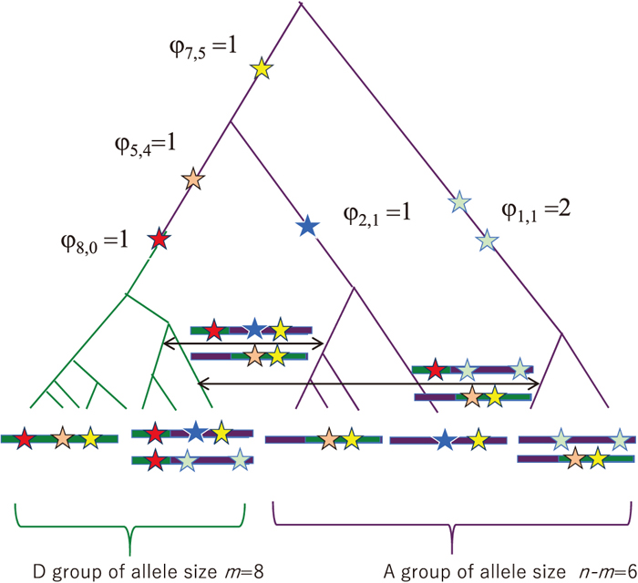
The 2D SFS is formulated to extract information about an incomplete selective sweep that is inscribed as biallelic SNPs in a genomic region sampled from a single panmictic diploid population. Two allele groups, the D group of size m (1 ≤ m < n) and the ancestral allele (A) group of size n−m where n is the entire sample size, are defined by the derived/ancestral state of a predetermined focal site or a core site, with the derived allele frequency being fr = m/n. These groups are extended to an LD region or a core region surrounding it (Fujito et al., 2018a). The 2D SFS for linked neutral polymorphism in the core region is denoted by the matrix {φi,j}, where the (i,j) element represents the number of segregating sites at which i (0 ≤ i ≤ m) derived alleles are found in the D group and j (0 ≤ j ≤ n−m) derived alleles are found in the A group. The total number of derived alleles is 1 ≤ k = i + j < n. We are concerned only with segregating sites in a sample and ignore φ0,0 and φm,n−m or set them to 0. φi,0 denotes the number of segregating sites at which i derived alleles can be found only in the D group. For 1 ≤ i < m and 1 ≤ j ≤ n−m, the presence of φi,j > 0 implies that, under the assumption of the infinite-sites model (Kimura, 1969), these segregating sites have experienced recombination. Note that when φi,n−m > 0, there are only three different types of gametes specified by the core site and a linked site, despite the fact that recombination between the sites is required to produce them. In other words, when we distinguish between the derived and ancestral alleles, the presence of four different types of gametes is not a necessary condition for the involvement of recombination.
The SFS can capture rich information about the SNP sites (Sawyer and Hartl, 1992; Bustamante et al., 2001). The entire distribution was used in the composite likelihood methods (Kim and Stephan, 2002; Nielsen et al., 2005; Williamson et al., 2007) as well as in inference methods about population demographic histories (Liu and Fu, 2015; Lapierre et al., 2017; Terhorst et al., 2017). However, the SFS is usually very sparse. As a 2D SFS is even more sparse, it is sensible and convenient to consider compressed versions simultaneously:
|
ξ
k
=
∑
i=0
k
φ
i,k-i
for 1≤k<n,
| (1a) |
|
ζ
i
=
∑
j=0
n-m
φ
i,j
=
φ
i,0
+
ζ
˜
i
for 1≤i<m,
| (1b) |
where
ξk and
ζi, with
φi,0 and
ζ
˜
i
=
∑
j=1
n-m
φ
i,j
, denote the one-dimensional (1D) SFS for the entire sample and the D group subsample, respectively.
In addition to the entire SFS, we consider various summary statistics, which include D by Tajima (1989), H by Fay and Wu (2000), E by Zeng et al. (2006), K instead of the original symbol L by Ferretti et al. (2017), and Fc by Fujito et al. (2018a, 2018b). However, if D, H, E and K are applied to the entire sample, the statistical power may be weakened in the present case of incomplete or partial selective sweeps. We therefore apply them to the D group subsample and re-evaluate their statistical behavior in this circumstance. The pattern and extent of polymorphism within the D group are the key features to be estimated for detecting incomplete selective sweeps. One such feature is captured by the Fc statistic, which can be rewritten in terms of {φi,j} as
|
F
c
=
∑i
φ
i,j
∑(
i+j
)
φ
i,j
.
| (2) |
Each summation is taken over all values of
i and
j in 0 ≤
i ≤
km, 0 ≤
j ≤ min(
n−
m,
km) and 1 ≤
i +
j ≤
km, where
km is the largest number of the
k =
i +
j derived alleles in the frequency class
cr−1. Here,
cr at a core site with
m derived alleles (
km <
m) is determined under the standard neutral model of constant size, hereafter referred to as the standard model (
Fujito et al., 2018a). In a sample of size 503 <
n < 1,367,
km takes one of 1, 3, 9, 25, 68, 185 and 503 in the seven possible frequency classes, with each having nearly equal numbers of segregating sites, and we set
cr = 1 if
m = 1,
cr = 2 if 1 <
m ≤ 3, etc. For the promoter region of
ST8SIA2 with
n = 1,008 and
m = 349 in the East Asian (EAS) population (1000GD), we set
cr = 7 from 185 <
m ≤ 503; thus,
km = 185 in class 6. Using
km, we can rewrite the denominator in
Formula (2) as
∑
k=1
k
m
k
ξ
k
.
The two vector components φi,0 and
ζ
˜
i
in Formula (1b) are most informative and convenient to describe IAV. We denote the maximum value of i by imax, which satisfies φi,0 > 0. φi,0 > 0 indicates two possibilities. One for a wide range of i with φi,0 > 0 (or a large imax) results from a soft sweep, wherein more than one distinct derived haplotype with respect to a core site has been subjected to positive selection since it began to act. As recombination is unlikely to generate φi,0 > 0 under the circumstances discussed in this study (see below), this would provide strong evidence for soft sweeps, regardless of the
ζ
˜
i
values. However, φi,0 > 0 for some i values may occasionally be created by the cumulative effects of recombination, genetic drift and insufficient sampling processes (Fig. 1). It is then necessary to examine if
ζ
˜
i
>0
holds, because it is an unambiguous sign of recombination with respect to the core site, as discussed above and in the four-gamete test (Hudson and Kaplan, 1985), and cannot be produced directly by any form of selective sweep. The rationale behind this is as follows. Suppose that a strong selective sweep is ongoing. Under this ideal situation, the genealogy among the derived alleles in the D group would be less structured with shortened basal branches, and their family size manifested by mutations would remain small in most cases. Recombination between the D and A groups can therefore make
ζ
˜
i
positive only for restricted i values in
1≤i≤
i
max
+
and
m-
i
max
-
≤i<m
, provided that these maximum family sizes (
i
max
±
) revealed by recombination are much smaller than m/2. The former case for
1≤i≤
i
max
+
can occur for mutations that originate from the A group, but are subsequently recombined with the derived core alleles. On the other hand, the latter case for
m-
i
max
-
≤i<m
can occur for mutations that are shared by all the lineages in the D group (Fig. 1). In either case, the recombining unit size must be identical to the number of descendant lineages of that recombining branch in the D group. Conversely, if a reciprocal relationship, such as
ζ
˜
i
=
ζ
˜
m-i
, is observed, it can be considered as a manifestation of the family size within the D group. Unfortunately, this exact relationship can be observed only when the population recombination rate of ρ = 4Ner is limited (Ne and r refer to the effective population size and the recombination rate per core region per generation, respectively). It is possible for
ζ
˜
m-i
>0
to be created even if i individual recombination events involve only singleton branches. As this is very unlikely for
ζ
˜
i
with small values of i,
ζ
˜
m-i
declines more slowly than
ζ
˜
i
as i increases. Therefore,
ζ
˜
i
with small values of i reflects the genealogical structure of IAV more accurately than the reciprocal
ζ
˜
m-i
. In addition, the absolute value of
ζ
˜
i
may differ greatly from that of
ζ
˜
m-i
because the relevant mutations involved are asymmetric in number, even within the same A group. In fact,
ζ
˜
m-i
>0
is produced only by mutations in the stem lineage of the D group, whereas
ζ
˜
i
>0
can be produced by a much wider range of mutations that have accumulated in the A group.
Overall, in the absence of recombination events, we have
ζ
˜
i
=0
exactly for 1 ≤ i < m, irrespective of the mode of selective sweep. Under a hard sweep, φi,0 > 0 is concentrated in a narrow range of 1 ≤ i ≤ imax, whereas under a soft sweep, φi,0 > 0 spreads over a wide range of i; however, there is a gray zone in between. In the presence of recombination,
ζ
˜
i
>0
under a hard sweep is generally concentrated in
1≤i≤
i
max
+
and
m-
i
max
-
≤i<m
because of the small family size within the D group. When
i
max
+
differs from
i
max
-
, we consider the larger one, denoted by
i
max
*
, as the
ζ
˜
i
-based estimate of the maximum family size within IAV. The size of imax and
i
max
*
under a soft sweep may be much larger than those under a hard sweep, and recombination augments this trend.
Based on the different implications of φi,0 and
ζ
˜
i
outlined above, we divide the total number of segregating sites (Sζ) within the D group into two components, Sζ0 and Sζ1, as follows:
|
S
ζ
=
∑
i=1
m-1
ζ
i
=
∑
i=1
m-1
φ
i,0
+
∑
i=1
m-1
ζ
˜
i
=
S
ζ0
+
S
ζ1
.
| (3a) |
used
Sζ to estimate the time elapsed since a selective sweep assuming a star-shaped genealogy, and
Satta et al. (2018) studied the nonequilibrium distribution of {
ζi} normalized in individual frequency classes
cr (1 ≤
cr ≤ 8, depending on the derived core allele frequency in the 1000GD). However, no-one has studied
φi,0 and
ζ
˜
i
or
Sζ0 and
Sζ1, separately. We also divide the total number of derived alleles (
Lζ) within the D group into two components,
Lζ0 and
Lζ1, as follows:
|
L
ζ
=
∑
i=1
m-1
i
ζ
i
=
∑
i=1
m-1
i
φ
i,0
+
∑
i=1
m-1
i
ζ
˜
i
=
L
ζ0
+
L
ζ1
,
| (3b) |
where
Lζ is the sum of the scaled SFS (
Fu, 1995) of
ζ
i
′
=i
ζ
i
within the D group and is expected to be small under strong selective sweeps. However, it is desirable to exclude the possibility of either background selection (
Charlesworth and Charlesworth, 2012 and references therein) or an intrinsically low population mutation rate in a core region (
θ = 4
Neu, where
u is the neutral mutation rate per region per generation). To have such internal control, we may also compute the number of derived alleles in the entire sample (
L
ξ
=
∑
k=1
n-1
k
ξ
k
) and use it to standardize the IAV components in
Formula (3b):
|
L
c0
=
L
ζ0
/
L
ξ
,
L
c1
=
L
ζ1
/
L
ξ
and
L
c
=
L
ζ
/
L
ξ
=
L
c0
+
L
c1
.
| (4) |
We emphasize that the unstandardized Lζ0 is also important. Under the assumption of a molecular clock, Thomson et al. (2000) and Tang et al. (2002) used Lξ/n as an estimator of the scaled TMRCA (utG = θTG, where TG = tG/4Ne) of a random sample of size n. We note that Lξ/n is the average number of mutations per lineage that have accumulated during tG generations. Hudson (2007) provided the variance formula,
V
u
t
G
, of utG. We can analogously estimate the scaled TMRCA (utD = θTD, where TD = tD/4Ne) of the D group from the average number of mutations per lineage (C) that accumulated during tD generations. However, it is essential to exclude recombinant SNP sites so that we define the estimator as follows:
Furthermore, following
Hudson (2007), we define its variance as
|
V
u
t
D
=
L
ζ0
m
-
m-1
m
θ
φ
2
,
| (5b) |
where
θ
φ
=
1
(
m
2
)
∑
i=1
m-1
i(
m-i
)
φ
i,0
is the pairwise mean number of the mutational differences at the non-recombinant SNP sites within the D group. If we write
B =
Lξ/
n −
C,
B becomes equal to the number of mutations that have accumulated in the stem lineage of the D group. Thus, an alternative estimate of
B is obtained by directly counting the number in the 2D SFS:
|
B=
∑
i=m-
i
max
-
m
∑
j=0
n-m
φ
i,j
=
∑
i=m-
i
max
-
m
ζ
i
.
| (6) |
We can use either
B +
C or
Lξ/
n as an estimate of
utG. Under the standard model, we expect
E{
Lξ} =
θ(
n − 1) (
Watterson, 1975;
Fu, 1995), where
E{ } is an expectation operator, and
E{
B +
C} =
θ(
n − 1)/
n. In
Formulae (5a and
b), we also note that
u differs from region to region because
u =
μl, where
μ is the mutation rate per site and
l is the length of a (core) region. The
ρ insensitivity of
utD and
V
u
t
D
is crucial when applied to autosomal regions. This property will be examined later by coalescent simulations.
Next, we are concerned with the average number of derived alleles per segregating site in three categories:
|
G
c0
=
L
ζ0
/
S
ζ0
,
G
c1
=
L
ζ1
/
S
ζ1
and
G
c
=
L
ζ
/
S
ζ
.
| (7) |
Provided that there is at least one segregating site in each category, these
G statistics are indices for the multiplicity of derived alleles per segregating site within the D group. In particular,
Gc0 can be referred to, by definition, as the average family size in the D group. All three categories should be small under a hard sweep if recombination is rare. Conversely, relatively large values of
Gc0 and
Gc1 signify a soft sweep and recombination, respectively. The expected value of
Gξ =
Lξ/
Sξ in the entire sample can be approximated by
E{
Gξ} ≈
E{
Lξ}/
E{
Sξ} for a large number of segregating sites, where
S
ξ
=
∑
k=1
n-1
ξ
k
. Using the standard model and by defining
a
n
=
∑
k=1
n-1
1/k
, we have
E{
Gξ} ≈ (
n − 1)/
an, which is greater than 100 for
n = 1,000, or each segregating site in this large sample is represented by more than 100 derived alleles on average. Thus, the
G statistics are rated “small” if they are much smaller than 100 in the 1000GD.
In addition to Gc0, we consider the following index of the IAV multiplicity:
|
γ(
i
m
)=
∑
i
m
m-1
φ
i,0
∑
i=1
m-1
φ
i,0
.
| (8) |
is based on the interpretation that the ratio of
ξ
i
/
∑
i=1
n-1
ξ
i
represents the probability of observing
i derived alleles at a segregating site in a sample of size
n (
Kim and Stephan, 2002;
Charlesworth and Charlesworth, 2012).
Gc0 is more sensitive to
φi,0 with large values of
i than
γ(
im), although
Gc0 and
γ(
im) are closely related. For a hard sweep with
fr = 0.6 or
m = 600 in a sample of size
n = 1,000,
γ(
im) = 0.1 will result in
im = 6, irrespective of
ρ, and
Gc0 may become about 6–7. However, both
Gc0 and
γ(
im) depend strongly on the number of singletons (
φ1,0). If there are too many singletons, these values are kept small, which is undesirable for distinguishing between hard and soft sweeps. Therefore, we also examine and may interchangeably use an alternative
γ
*
(
i
m
)
that excludes
φ1,0 from the definition given in
Formula (8). Under the standard model, we have
E{γ(
i
m
)}≈(
a
m
-
a
i
m
)/
a
m
and
E{
γ
*
(
i
m
)}≈(
a
m
-
a
i
m
)/(
a
m
-1)
, which become 0.59 and 0.69, respectively, if
im = 10 and
m = 600. Similarly, we examine
G
c0
*
that excludes singletons while calculating
Gc0. As a soft sweep is defined by the presence of more than one distinct lineage (or haplotype) in the D group, we may impose a criterion in terms of relatively large values of
γ*(10) and
G
c0
*
.
Many inference procedures for selective sweeps are based on differences among the unbiased estimators of θ (Tajima, 1989; Fay and Wu, 2000; Zeng et al., 2006, 2017; Ferretti et al., 2017). Under the standard model, we can obtain an estimate of θ as θs = ξ1 from the observed number of singletons (Fu and Li, 1993; Fu, 1995) or one of the following formulae:
|
θ
w
=
1
a
n
∑
k=1
n-1
ξ
k
,
| (9a) |
|
θ
π
=
1
(
n
2
)
∑
k=1
n-1
k(n-k)
ξ
k
,
| (9b) |
|
θ
L
=
1
n-1
∑
k=1
n-1
k
ξ
k
,
| (9c) |
|
θ
H
=
1
(
n
2
)
∑
k=1
n-1
k
2
ξ
k
.
| (9d) |
Among six possible pairwise combinations of the four estimators in
Formulae (9), four difference statistics have been proposed:
|
D
ξ
=(
θ
π
-
θ
w
)/
N
D
(
S
ξ
),
| (10a) |
|
H
ξ
=(
θ
π
-
θ
H
)/
N
H
(
S
ξ
),
| (10b) |
|
E
ξ
=(
θ
L
-
θ
w
)/
N
E
(
S
ξ
),
| (10c) |
|
K
ξ
=(
θ
w
-
θ
H
)/
N
K
(
S
ξ
).
| (10d) |
(
Sξ) is the standardizing coefficient, which can be expressed as follows:
|
N
Ω
(
S
ξ
)=
λ
n
S
ξ
+
κ
n
S
ξ
(
S
ξ
-1)
,
| (10e) |
with
λn and
κn specific to the Ω statistic (Table 4 in
Ferretti et al., 2017, but with the numerator
n − 2 in
κ
n
D
being read as
n + 2, as in
Tajima, 1989). To quantify IAV based on these statistics, we simply replace
ξk by
ζi and
n by
m in
Formulae (9) and
(10). We denote the latter as
Dζ,
Hζ,
Eζ and
Kζ. Under a hard sweep and in the absence of recombination, it is expected that
θw >
θπ >
θL >
θH, and therefore,
Dζ < 0,
Eζ < 0,
Hζ > 0,
Kζ > 0. However, the mode of selective sweeps and the presence of recombination can greatly alter these expectations.
The case of ST8SIA2
Before going further, let us exemplify these statistics with actual data: the promoter region of the EAS ST8SIA2 locus (Fujito et al., 2018a, 2018b). The core site consists of three promoter SNPs and divides the whole sample into CGC and non-CGC haplotype groups. The core region is ca. 15 kb long (Chr 15, 92924515–92939701 in GRCh37), which is 1–3 kb shorter than that in the previous study (Fujito et al., 2018a) because of the exclusion of apparent recombinant sites located near the 5’ and 3’ ends. For the EAS sample in the 1000GD, we obtained the following values: Sζ = 30, Fc = 0.013, Lc = 0.09 (Lc0 = 0.002, Lc1 = 0.088), Gc = 47.0 (Gc0 = 1.52, Gc1 = 153), θw = 4.67, θπ = 0.39, θL = 4.05, θH = 7.71, Dζ = −2.47, Hζ = −4.52, Eζ = −0.30 and Kζ = −0.93. We also obtained a small maximum family size of imax = 4 from φ4,0 = 1 and φi>4,0 = 0 or γ(im) = 0 for im ≥ 5, demonstrating the reduced IAV in this genomic region. Consistent with these findings, the number of segregating sites (Sζ) within the CGC haplotype group is much smaller than Sξ = 132 in the entire sample. All the observed values of Fc, Lc0, Gc0 and Dζ are small at highly significant levels of P < 0.001 in the simulated standard model. We observed that the small Fc value results in part from the exclusion of the derived alleles that belong to cr = 7, or more precisely in the frequency range of
m-
i
max
-
≤i<m
in Formula (2). If they had been included, Fc would have been as large as Lc. Therefore, the exclusion procedure in Fc is legitimate because these derived alleles originated in the A group and were deceptively incorporated into the IAV by recombination. The Gc1 and Lc1 ≈ 40Lc0 values show significant effects of recombination on the IAV. The negative Dζ and Hζ values are potentially useful to quantify an incomplete selective sweep, even though Dξ and Hξ for the entire sample lack their statistical powers (Table S5 in Fujito et al., 2018a). Dζ < 0 reflects an excess of rare alleles and a lack of intermediate frequency alleles. Hζ < 0 reflects a lack of intermediate frequency alleles and an excess of high frequency alleles. In the present case, an excess of high frequency alleles results from recombination, unlike their gradual increase toward fixation by positive selection. This is reflected in
ζ
˜
i
>0
for
m-
i
max
-
≤i<m
with
i
max
-
=3
. Finally, the selective sweep for the CGC haplotype group is so strong and recent that we may estimate the TMRCA (tD = C/μl) of the CGC group as 12.2 ± 3.9 thousand years (ky) from C = 32/349 = 0.092, the mutation rate per site per year of μ = 0.5 × 10⁻⁹ (Scally and Durbin, 2012), and θφ = 0.183 (B = 18 and Lξ/n = 15.6, a slightly smaller value than B + C). Although the CGC haplotype originated in Africa long ago, positive selection began to exert pressure on a single ancestral haplotype lineage in East Asia around 12 ky ago (Fujito et al., 2018b). Therefore, the core region of ST8SIA2 provides a solid example of a hard sweep using standing variations (Przeworski et al., 2005; Schrider and Kern, 2016), namely hardening soft sweeps (Wilson et al., 2014).
SIMULATED 2D SFS
Modes of selective sweeps and effects of recombination
We present a simulated 2D SFS in Supplementary Fig. S1 for a small sample of n = 68, under the conditions of the presence or absence of recombination and hard or soft sweeps for the D group (ms by Hudson, 2002; discoal by Kern and Schrider, 2016). The methods for testing neutrality and examining statistical power are the same as described in Fujito et al. (2018a) and are not repeated here. An alternative representation of {φi,j}, as presented in Table 1, demonstrates that in the absence of recombination, only φi,0, φ0,j and φm,j elements can have non-zero values, or polymorphism is represented only by the three edges of the matrix {φi,j}. This is because the D group is always monophyletic with respect to the A group and φi,n−m = 0 holds true for all possible values of i. Conversely, the presence of only three different types of gametes along with φi,n−m > 0 is a definite indication of recombination. If the D and A groups are reciprocally monophyletic, we also expect φm,j = 0 for 1 ≤ j < n−m. In any case, the D and A groups evolve “independently” in the absence of recombination. It is recombination that generates the SNP sites with
ζ
˜
i
=
∑
j=1
n-m
φ
i,j
>0
for some values of i in 1 ≤ i < m and requires a 2D SFS to completely describe the pattern and level of polymorphism for incomplete selective sweeps.
Table 1. Compressed expression of a 2D SFS for the non-zero elements of the matrix {
φi,j}
| i | j | k | φi,j |
|---|
| 0 | 1 | 1 | 76 |
| 1 | 0 | 1 | 8 |
| 0 | 2 | 2 | 29 |
| 0 | 3 | 3 | 61 |
| 3 | 0 | 3 | 3 |
| 0 | 4 | 4 | 7 |
| 0 | 5 | 5 | 2 |
| 5 | 0 | 5 | 1 |
| 0 | 6 | 6 | 2 |
| 0 | 7 | 7 | 1 |
| 0 | 10 | 10 | 7 |
| 0 | 13 | 13 | 111 |
| 34 | 0 | 34 | 5 |
| 34 | 2 | 36 | 7 |
| 34 | 8 | 42 | 11 |
| 34 | 18 | 52 | 4 |
| 34 | 21 | 55 | 100 |
For a selective sweep, we used discoal (Kern and Schrider, 2016) for n = 68, m = 34, θ =100, a = 2Nes = 400, fr = 0.5 and ρ = 0. The subscripts i and j represent the numbers of derived alleles in the D and A groups, respectively, and k = i + j.
Figure 2 shows that for hard sweeps, the expected values of φi,0 and
ζ
˜
i
divided by the number of their respective singletons decrease more rapidly than those of 1/i expected in the standard model (Fu, 1995) as i increases. φi,0 and
ζ
˜
i
are subcritical, and they indicate that alleles in the D group do not manifest large family sizes of lineages that share particular mutations. The declining pattern of
ζ
˜
i
depends on the recombination rate ρ. Contrastingly, φi,0 is almost unchangeable by recombination. This remarkable robustness results from the fact that although recombination may occasionally contribute to φi,0 > 0, its effect is restricted to i in 1 ≤ i ≤ imax for some small number of imax. In fact, φi,0 > 0 for large values of i can be realized only by particular mutations in an ancestral recombination graph (Griffiths, 1991; Griffiths and Marjoram, 1997) together with fortuitous loss or no sampling of recombinant haplotypes in the A group. Under ordinary circumstances, φi,0 therefore remains unaffected even by frequent recombination. Thus, tD and the variance in Formula (5) are also insensitive to recombination under selective sweeps (Supplementary Fig. S2). However, recombination dramatically increases
ζ
˜
i
for
1≤i≤
i
max
+
and
m-
i
max
-
≤i<m
(Fig. 2). Although
ζ
˜
i
>0
in the two opposite ranges of i is somehow related to the genealogical structure of IAV, the outcome may suffer from repeated occurrences of recombination, thereby no longer reflecting the structure accurately. In fact,
ζ
˜
i
>0
for
m-
i
max
-
≤i<m
can occur much more frequently than 1/i, irrespective of fr, indicating that it is related to the recombination processes between the D and A groups and not the coalescent processes with mutations within the D group.

To further quantify φi,0,
ζ
˜
i
and their related summary statistics, we performed extensive coalescent simulations. The results of these simulations are summarized semi-quantitatively in Table 2, which gives the empirical criteria to evaluate the significance of sweep signals, classify the mode of selective sweep, and assess the effects of recombination. The family size is independent of ρ, as it should be, but is strongly dependent on the mode and strength of the selective sweeps. Supplementary Table S1 presents 18 summary statistics for IAV under hard sweeps when θ = 20, n = 1,000, a = 2Nes = 500 (s: genic selection intensity), and fr = 0.3, 0.6 and 0.9. As mentioned above, φi,0 is insensitive to ρ and so are the related Sζ0, Lζ0 and Gc0. In contrast, none of the four ζ-based estimators of θ are insensitive to ρ. This sensitivity is also reflected in Hζ, Eζ and Kζ, all of which can take positive and negative values as ρ changes. However, there is an exception to this large fluctuation. Dζ can keep a negative value within the examined parameter range because it depends on θw and θπ, and not on θL and θH, which are much more sensitive to ρ than the former two. In other words, recombination generates superficial signals on θL and θH through
ζ
˜
i
>0
for large values of i. These results suggest that we cannot use Hζ, Eζ or Kζ without knowing the accurate values of ρ in actual data analyses.
Table 2. Semi-quantitative criteria for detecting and classifying incomplete selective sweeps and evaluating the significance of recombination effects
| Level | IAV
Multiplicity |
ζ
˜
i
=0
for all
values of i
Lc1 and Gc1 = 0 |
ζ
˜
i
>0
for some
values of i
Lc1 > 0 and Gc1 > 0 |
|---|
Low
Fc « 1
Lc0 « 1
Relatively high | Small imax
γ*(10) < 0.1
G
c0
*
<9
| Hard sweep
No recombination | Hard sweep
Recombination |
Large imax
0.1 <γ*(10)
9≤
G
c0
*
| Soft sweep
No recombination | Soft sweep
Recombination |
Figure 3 shows the receiver operating characteristic (ROC) curves comparing the sensitivity (true-positive rate or power, 1 − β) and 1 – specificity (false-positive rate, α) of Fc, Lc, Lc0, Gc and Gc0, as well as those of Dζ, Hζ, Eζ and Kζ. The former five are tested in left-tailed tests and the latter four are tested in two-tailed tests (Fig. 2 in Ferretti et al., 2017). Each ROC curve was constructed from 1,000 simulations under strong selection (a = 500) and 1,000 simulations under near neutrality (a = 1, f0 = 0.5 and fr = 0.6) to facilitate random sampling of the derived alleles with a specified frequency (fr). Thus, our ROC curves are conservative compared to those when pure neutrality is assumed as a null hypothesis, and a comparison between pure neutrality (by ms) and near neutrality (by discoal) indicates visible effects of a = 1 on the 2D SFS (Supplementary Fig. S3). The area under an ROC curve, often denoted as AU(RO)C, measures the discriminative ability of a statistic. For hard sweeps (Fig. 3A) and with ρ = 0, Fc, Lc0 and Gc0 can discriminate the hypotheses well and may be categorized as excellent, as a rule of thumb. Among the four difference statistics, Dζ outperforms Hζ, Eζ and Kζ. However, if ρ = 50, Lc0 and Gc0 outperform Fc, while Hζ and Kζ outperform Eζ and Dζ. Recombination reduces the power of Fc because this statistic is not completely free from the effects of recombinant haplotypes. This is also reflected in the relatively low power of Gc and Lc. The powers of Hζ, Kζ and Eζ become even greater when ρ = 50 than when ρ = 0. This unexpectedly enhanced power results from the increased values of ζi for large values of i because of the high recombination rate. Overall, for hard sweeps, (i) it is possible to infer the maximum and average family sizes among D group lineages; (ii) to evaluate IAV, it is recommended to use φi,0 and closely related summary statistics, such as Gc0, Lc0 and Fc; and (iii) the power of some difference statistics is extremely sensitive to recombination, and, thus, caution is required when interpreting the application results. Regarding (iii), an alternative may be to recalculate the difference statistics based on φi,0 rather than ζi.

A soft sweep can be modeled by a high initial frequency of the D group, such as f0 = 0.1 (Ferrer-Admetlla et al., 2014; Kern and Schrider, 2016), and it generates SNP sites with φi,0 > 0 for multiple intermediate values of i. Although effects of recombination on the pattern of
ζ
˜
i
are similar to those of hard sweeps, IAV for soft sweeps can be considerably high such that φi,0 and
ζ
˜
i
spread broadly in the 1 ≤ i < m range. For the soft sweep in Fig. 2B and in a specified range of 1 ≤ i ≤ 30, for example, we observed γ(10) ≈ 0.18 for ρ = 50, 20 and 0. These values are significantly larger than those for the hard sweeps shown in Fig. 2A, i.e., γ(10) ≈ 0.03 for ρ = 50, 20 and 0. Supplementary Table S2 presents the 18 statistics for soft sweeps. As mentioned above, φi,0-related statistics are remarkably robust to recombination, although this does not guarantee their ability to identify soft sweeps. In fact, the absolute values are substantially larger than those for the corresponding hard sweeps. With increased φi,0 and
ζ
˜
i
for intermediate values of i, all other statistics are significantly affected. The ROC curves for f0 = 0.1, fr = 0.6 and ρ = 0 (Fig. 3B) show lower discriminative abilities of Fc, Lc0 and Gc0 and almost no power of Dζ, Hζ, Eζ and Kζ for low cutoff values. Detecting soft sweeps strongly depends on the typically unknown parameter f0. If we reduce the value of f0 from 0.1 to 0.05, the powers of some statsitics are recovered. If we increase the value of fr from 0.6 to 0.9, the powers of some statistics are recovered as well.
The duration time (T) of the selected phase in our simulation is approximately given by
T=
1
a
ln
(1-
f
0
)
f
r
f
0
(1-
f
r
)
in units of 4Ne generations (Kern and Schrider, 2016): T = 2.60/a for f0 = 0.1 and fr = 0.6, 3.35/a for f0 = 0.05 and fr = 0.6, and 4.39/a for f0 = 0.1 and fr = 0.9. All these duration times are shorter than 0.01 if a ≥ 500. Considering that
T=
t
4
N
e
=
ut
θ
and
T
D
=
u
t
D
θ
in Formula (5a), we may use them to formally redefine the hard and soft sweeps. A selective sweep would be hard if TD ≤ T (tD ≤ t), and vice versa. Similarly, a selective sweep would be soft if TD > T (tD > t), or, equivalently, if more than one distinct ancestral lineage is assured beyond T, and vice versa. The frequency change of the D group depends on the strength and mode of selection (Wilde et al., 2014), and the same is true for T and TD. T is a major factor that affects the power of a statistic wherein f0 becomes a more crucial determinant than fr (for the case of fr = 1, see Innan and Kim, 2004; Przeworski et al., 2005). The increased extent of the power varies largely among the statistics used, i.e., Fc, Lc0 and Gc0 are rather robust to changes in f0 and fr, whereas Dζ and Eζ are sensitive, but Hζ is insensitive. Generally, the power of detecting soft sweeps of f0 = 0.1 by a single SFS statistic may not be sufficiently high for a given low false-positive rate α. Readers may refer to Nielsen et al. (2005), Zeng et al. (2006, 2007), Grossman et al. (2010), Ayub et al. (2013), Sheehan and Song (2016) and Schrider and Kern (2017) for improved methods that combine several population genetic summary statistics and related issues.
Past incomplete selective sweeps
Any method would lose the ability to reject the null model in favor of a selective sweep with the time (τ in units of 4Ne generations) elapsed since the fixation of a beneficial allele (Simonsen et al., 1995; Kim and Stephan, 2002; Przeworski, 2003). As sweep signals dissipate rapidly due to new mutations and recombination, the detectable period τ of a selective sweep may not greatly exceed 0.1 (Przeworski, 2003; Ferretti et al., 2017). In the case of modern humans, this may amount to 4,000 generations or 105 years if Ne = 104 and the generation time is 25 years. Similarly, we are concerned with the possibility that positive selection would cease before a selective sweep is completed, presumably because of the ever-changing physical and/or cultural environment. We want to determine the smallest value of τ that can be statistically distinguishable from τ = 0 (ongoing sweep) and the statistic that is most suitable for this distinction. If τ > 0, the condition for a past hard sweep becomes TD ≤ T + τ, and that for a past soft sweep becomes TD > T + τ. During the time period of τ (forward in time), the D group frequency changes from fr to fr(τ) by genetic drift. Therefore, in a sample taken at τ, we observe the D group alleles with a number that may differ greatly from nfr = m and may range from 0 (loss) to n (fixation in the sample). Theoretically, a large number of coalescent events can occur even during a time period as short as τ = 0.05. Tavaré (1984) and Takahata and Nei (1985) derived two seemingly different formulae for the probability gn,k(2τ) of the number (k) of distinct ancestors 2τ units of time ago in a sample of size n wherein time τ is measured in units of 2Ne generations (Chen, 2012 for the case of time-varying population sizes). Wakeley (2009) highlighted their equivalence, provided that the denominator in his formula (3.42) is read as k!(i – k)!n(i) rather than i!(i – k)!n(i). gn,k(2τ) with n = 100 or more shows that k at τ = 0.05 would be concentrated between 15 and 25 (Supplementary Fig. S4), thereby suggesting that these post-sweep coalescences substantially alter IAV.
We examined Fc, Lc0, Gc0 and Dζ to determine how their ability to detect ongoing selective sweeps declines with τ, and we measured their power at τ = 0.01, 0.03 and 0.05 when a type I error rate α was specified as 0.01. Figure 4 shows that for hard sweeps, the Fc power fades most rapidly, followed by Lc0. However, the Gc0 power remains high for a relatively long time, and the Dζ power exbihits a complicated pattern. The primary change in these statistics results from the newly created φi,0 > 0 for the relatively large values of i or increased imax due to coalescence in an elongated neutral phase of a post-sweep (Supplementary Fig. S5). Sζ0 and Lζ0 increase proportionally with τ, as does Lc0 = Lζ0/Lξ; however, Gc0 = Lζ0/Sζ0 increases more slowly and retains its power for a relatively long time. It is rather unexpected that Gc0 does not easily distinguish between ongoing and past selective sweeps. In contrast, as the power of Fc reduces to 50% or less even at τ = 0.01, it would be most useful to evaluate if τ > 0. The presence of recombination enhances this decline dramatically.
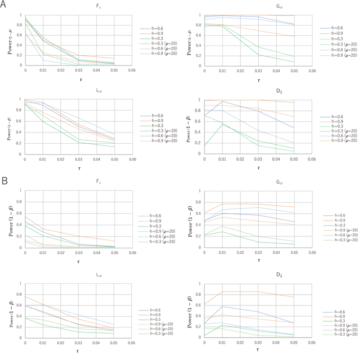
Overall, if we observe significantly small values of Fc, Lc0 and Gc0 together with small values of imax and γ(im), we identify an ongoing hard sweep. If we observe significantly small values of imax, γ(im) and Gc0 but relatively large values of Fc as compared to Lc0, we identify a past hard sweep. The same conclusions are applied to the case of soft sweeps (Fig. 4). However, the powers of Fc, Lc0, Gc0 and Dζ for soft sweeps may be low even at τ = 0 and approach the specified level of α rapidly with τ. In hard and soft sweeps, recombination plays a significant role in diminishing the powers of Fc and Dζ, whereas Gc0 and Lc0 are somewhat resistant.
APPLICATIONS TO HUMAN GENOMES
A genomic landscape revealed by 100 intronic SNPs
In this section, we render a genomic landscape with a 2D SFS, although it is not exhaustive. By filtering biallelic SNP sites in the 1000GD by autosomal introns and Global MAF (ca. 40%), we randomly chose >100 core sites, and examined LD and 2D SFS in the EAS population (see Supplementary Table S3 for their SNP reference sequence (rs) numbers). To facilitate the determination of a core region for each core site, we used a distance similar to the “half length” of LD (Reich et al., 2001), which is the distance from a core site at which LD drops below 1/2. However, we assumed a more tightly linked core region than expected by the half length. For this, we used r2 (Hill and Robertson, 1968), took the average over SNP sites with frequencies greater than 0.1fr in a 1-kb non-overlapping window, and determined the distance at which the averaged r2 value drops below 3/4. Two such distances on both sides of a core site mark the boundaries of the core region. The size determined in this way varies greatly among the core regions. In many cases, the averaged r2 value decreases below 3/4 even in the first 1-kb window from a core site (for instance, rs1484214), and in other cases it extends over a 150-kb region (for instance, rs7541057). In total, we excluded 45 sites with <1-kb core regions and added the same number of sites to keep the total number of 100 core sites. We confirmed that those 45 excluded SNPs do not show any signals of selective sweeps.
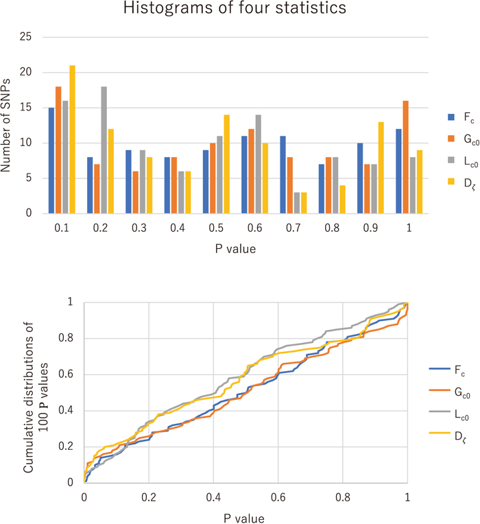
Assuming near neutrality of the 100 core variants, no recombination within a core region, and the nonequilibrium demography of Schaffer et al. (2005), we computed the P values of Fc, Lc0, Gc0 and Dζ, and examined the uniformity of their distributions by the chi-squared and Kolmogorov-Smirnov (KS with n = 100) tests as well as other multiple testing approaches (Fig. 5). The distribution for Fc is fairly uniform and does not reject any core site (
χ
df=9
2
=5.0
with P ≈ 0.8 and gmax = 0.089 with P > 0.05 in the KS test). Similarly, we obtained
χ
df=8
2
= 13.95
(P > 0.05) and gmax = 0.144 (0.05 > P > 0.01) for Lc0,
χ
df=9
2
=15.0
(P < 0.05) and gmax = 0.106 (P > 0.05) for Gc0, and
χ
df=7
2
= 19.1
(P < 0.01) and gmax = 0.151 (0.05 > P > 0.01) for Dζ. Thus, there are some indications against the null hypothesis. The multiple testing of Fc, Lc0, Gc0 and Dζ (Benjamini and Hochberg, 1995) consistently rejects zero, five, eight and eight core sites, respectively, with a 10% false discovery rate (FDR). Such different performances among the statistics result partly from their different sensitivities to recombination. The least sensitive are Gc0 and Lc0, the second least sensitive is Fc, and the most sensitive is Dζ. If Lc0, Gc0 and Dζ are used, at most one core site is erroneously rejected and the remaining four to seven support false null hypotheses. Thus, with a 10% FDR,
137~140
145
=95~97%
of intronic variants in human genomes are consistent with selective neutrality (Kimura, 1968). We also applied the same multiple testing to Fisher’s combined P values of Fc, Lc0 and Gc0, and obtained 10 loci for P < 0.01. This is consistent with the result of the independent tests, but it is overstated because of positive dependence among the three statistics. Regarding the proportion π0 of the true null hypotheses among all the hypotheses (Storey and Tibshirani, 2003; Benjamini et al., 2006), we estimated π0 to be 0.90 from the multiple testing and histogram (Fig. 5). The most significant deviation from neutrality is observed at an intron variant C/T (rs1587725) that is located in a serine/threonine kinase 32 (STK32B) and associated with an autosomal recessive skeletal dysplasia. The C frequency in the African population is < 12%, but approximately 80% in the non-African populations.
It is worth noting that these conclusions are based on the null hypothesis, which assumes the absence of recombination in addition to neutrality. Recombination affects the distributions of Fc, Lc0, Gc0 and Dζ by decreasing Sζ0 and contrastingly increasing Sζ1 in IAV (Supplementary Fig. S6). Although such effects of recombination are small for the case of selective sweeps with low levels of IAV, they can be substantial for the case of neutrality with relatively high levels of IAV. In the case of neutrality, recombination increases the expected values of Fc and Dζ so that their observed values become relatively small. For the same reason, recombination decreases the expected values of Lc0 and Gc0 or makes the distributions skew toward 0. Thus, in the presence of recombination, Fc- and Dζ-based tests become too sensitive, but Lc0- and Gc0-based tests become conservative. It is difficult to choose an appropriate recombination rate when testing a null hypothesis. However, the fact that the P values of the four statistics are approximately uniformly distributed under the null hypothesis of no recombination suggests that the effect of recombination is not substantial in the core region with r2 ≥ 3/4 despite a large number of segregating sites that indicate recombination. Simulated r2 values for various recombination rates are presented in Supplementary Fig. S7.
Six selected regions
We also examined six genomic regions encompassing the genetic loci of lactase (LCT) (Enattah et al., 2002; Tishkoff et al., 2007), ectodysplasin A receptor (EDAR) (Sabeti et al., 2007; Fujimoto et al., 2008; Kimura et al., 2009; Kamberov et al., 2013), abnormal spindle-like microcephaly (ASPM) (Evans et al., 2005), microcephalin-1 (MCPH1) (Mekel-Bobrov et al., 2005), neuregulin-1 (NRG1), and a disintegrin and metalloproteinase domain17 (ADAM17) (Pickrell et al., 2009). We selected these regions as representatives to test the power of our statistics. The six regions include two well-established cases, LCT (rs4988235) and EDAR (rs3827760), for positive selection, and two controversial cases, ASPM (rs41310927) and MCPH1 (rs930557), in relation to an LRH-based outlier approach (Yu et al., 2007) as well as allelic surfing (Currat et al., 2006). Further, to extend our previous study on ST8SIA2 (Fujito et al., 2018b), the regions include NRG1 (rs3924999) and ADAM17 (rs2709591), which are variants that are known to be associated with the risks of schizophrenia and various psychiatric phenotypes (Pickrell et al., 2009). The six core regions were determined in the same way as described in the 100-intron genomic landscape (Supplementary Fig. S8) and the observed values of several statistics are summarized in Table 3. First, we examined the level of the IAV through Fc and Lc0, the multiplicity through γ*(im) and
G
c0
*
, and the roles of recombination through Gc1 and Lc1 (Table 2). The P values were computed in the null hypothesis of pure neutrality in the nonequilibrium demographic model of the EAS or European (EUR) population (Schaffner et al., 2005) with the number of segregating sites being fixed to an observed one. Second, we estimated the TMRCA (tD) in the D group from the observed C value, the mutation rate μ, and the 3/4 length (l) core region.
Table 3. IAV statistics for
LCT and
ASPM in EUR (
n = 1,006) and for
EDAR,
MCPH1, NRG1 and
ADAM17 in EAS (
n = 1,008) in the 1000GD
| Loci (sweep mode) m (l) | LCT (hard)
511 (100 kb) | EDAR (hard)
880 (65 kb) | ASPM (NS)
413 (165 kb) | MCPH1 (soft)
770 (32 kb) | ADAM17 (soft)
871 (26 kb) | NRG1 (NS)
765 (3 kb) |
|---|
| Sζ0, Sζ1 | 66, 10 | 223, 67 | 279, 78 | 196, 92 | 111, 19 | 10, 3 |
| Lζ0, Lζ1 | 84, 2056 | 529, 33805 | 1394, 15348 | 785, 40146 | 561, 7840 | 19, 761 |
| Fc | 0.0054*** | 0.257* | 0.123 | 0.103** | 0.229* | 0.070 |
| Lc0 | 0.0015*** | 0.0091*** | 0.013 | 0.013** | 0.023** | 0.010 |
| imax | 6*** | 48*** | 187 | 85*** | 213 | 7 |
| γ*(10),
G
c0
*
| 0***, 2.8*** | 0.08***, 5.5*** | 0.33, 13 | 0.27, 10.2** | 0.31, 13.5** | 0, 3.3 |
The P values of Fc, Lc0, imax, γ*(10) and
G
c0
*
for each gene were obtained by ms (Hudson, 2002) using the observed Sξ value and demographic model by Schaffner et al. (2005); *** P < 0.001, ** 0.001 ≤ P < 0.01, * 0.01 ≤ P < 0.05 (see Supplementary Table S3 for the full table). NS: no evidence for a selective sweep.
For LCT in the EUR population, the core region became l = 100 kb long (Chr 2, 136608646–136708564). If we instead use the 1/2 length, the core spans a 600-kb genomic region. When l = 100 kb, there are 76 segregating sites within the D group, which are 14% (< fr = 51%) of the total in the same region. The IAV level is very low and provides the strongest evidence for a selective sweep. The estimated maximum and average family sizes are so small that the majority of the Sζ0 = 66 sites are singletons (
G
c0
*
<3
), and there is no segregating site with a multiplicity as high as 10 ≤ i or γ(10) ≤ γ*(10) = 0. Thus, the IAV in the T-13910 group—100% association with lactase persistence in the Finnish population—is unambiguously classified as an ongoing hard sweep (Table 2; Peter et al., 2012; Ronen et al., 2015). Nevertheless, there are additional Sζ1 = 10 segregating sites and Lζ1 = 2,056 derived alleles that are linked to the D group by recombination. This non-negligible effect of recombination is quantified by Gc1 and Lc1. Further, we obtained tD = 3,280 ± 480 years from C = 0.16 as well as
V
u
t
D
=5.7×
10
-4
with θφ = 0.33 (B = 52 and Lξ/n = 55.8, a slightly larger value than B + C). As mentioned earlier, this estimate of tD for a hard sweep provides a lower bound of the time period (t) of the selected phase. The simulation showed that t can be much longer than tD (data not shown). Our estimate of tD is as short as a recent onset of positive selection in Bronze Age Europeans (Allentoft et al., 2015), shorter than 4,000 years based on ancient DNA (Mathieson et al., 2015), much shorter than 7,500 years based on the ABC approach (Itan et al., 2009), but within a wide range of allele ages roughly estimated by LRH conservation (Bersaglieri et al., 2004).
We chose the core site of EAS EDAR at the nonsynonymous variant site 1540. The 3/4 length core region becomes 65 kb long, while the 1/2 length core region spans a region of > 500 kb (Chr 2, 109465127–109530021). There are 290 segregating sites within the high-frequency D group (fr = 0.87), which are about 59% of the total in the same region. The IAV level is as low as Lc0 = 0.0091, but Fc = 0.257 is higher than 0.196 in our previous estimate based on a different core region (Fujito et al., 2018a). The IAV multiplicity with imax = 48,
G
c0
*
≈5.5
, and γ*(10) < 0.1 is low, but higher than that in LCT. Including the two sites with i = 120 and j = 48, and with i = 384 and j = 17, the family size in the D group is fairly large, and recombination apparently plays a substantial role in increasing Gc1 and Lc1. From C = 0.60 and θφ = 1.19 (B = 58 and Lξ/n = 58.3, in agreement with B + C), we estimated tD ≈ 18.5 ± 2.5 ky. The derived core allele may not have originated in the main ancestral populations of East Asians (Mathieson et al., 2015). Yet all these features are best classified as a hard sweep that has been operating at least over the past 18.5 ky (t > tD).
The core region of ASPM in the EUR population is 165 kb long (Chr 1, 196990327–197155021). As this region is more than five times longer than that in our previous analysis (Fujito et al., 2018a), it includes a large number of segregating sites in the D group. The IAV level is inflated in terms of Lc0 and Fc. The IAV multiplicity is accordingly high and exhibits a fairly large family size (imax = 187,
i
max
*
=143
,
G
c0
*
≈13
, and γ*(10) ≈ 0.33). Despite the relatively low frequency, fr = 0.41, significant roles of recombination are apparent. These features are consistent with previous work (Yu et al., 2007) that showed that the region is not identified empirically as an outlier in the LRH test. The estimates of C = 3.38 and θφ = 5.91 (B = 113 and Lξ/n = 106, a slightly smaller value than B + C) led to tD ≈ 41 ± 7.9 ky.
Some genetic variants of the MCPH1 gene rapidly increased their frequencies in Eurasia. The 3/4 length core region in the EAS population is 32 kb long (Chr 8, 6286532–6318958) and there are 288 segregating sites (65% of the total) in the D group that show significantly low levels of Fc and Lc0 However, the core region exbihits relatively large family sizes (imax = 85,
i
max
*
=76
,
G
c0
*
≈10
, and γ*(10) = 0.27) and abundant recombinant haplotypes. These features are classified as an ongoing soft sweep with signficant effects of recombination. From C = 1.0 and θφ = 2.0 (B = 64 and Lξ/n = 61.7, a slightly smaller value than B + C), we have t < tD = 62.5 ± 13.2 ky, indicating that the selection began to operate after the major out-of-Africa dispersal (Bae et al., 2017; Mondal et al., 2019). However, in the EUR population, the IAV pattern and level differ significantly. The core region becomes 30 kb long (Chr 8, 6284798–6309364), and it shows a high IAV level and multiplicity with large values of Fc and Lc0 as well as those of imax = 802,
i
max
*
=9
,
G
c0
*
≈141
, and γ*(10) = 0.47. imax has the largest possible value when m = 803, and even if this φ802,0 = 4 is excluded, there still exist four sites of φ801,0 = 3, φ458,0 = 1, φ343,0 = 1, and φ340,0 = 1. The estimate of C = 8.7 in the D group (θφ = 2.35, B = 37 but Lξ/n = 37.3) shows tD = 580 ± 180 ky, which corresponds to a time much earlier than the origin of modern humans (Bae et al., 2017). There is no indication of any selective sweep for the MCPH1-derived allele at rs930557 in the EUR population.
ADAM17 converts NRG1 to its active form in the NRG-ERBB4 signaling pathway, and both genomic regions exhibit iHS selection signals in the EAS population (Pickrell et al., 2009). The core region of ADAM17 is 26 kb long (Chr 2, 9490015–9515668). The IAV level is low in terms of Fc and Lc0, but the IAV multiplicity is high (imax = 213,
i
max
*
=3
,
G
c0
*
≈13.5
, and γ*(10) = 0.31). The large value of imax results from the single occurrence of φ213,0 = 1. If that is excluded, the value of imax drops substantially, but is still as large as 48. These features may well be classified as an ongoing soft sweep. Using C = 0.64 and θφ = 1.16 (B = 24 and Lξ/n = 24.3, in agreement with B + C), we have tD = 49 ± 20 ky (> t). On the other hand, the core region of NRG1 in the EAS population becomes only 3 kb long (Chr 8, 32451286–32454158), the shortest among the six genes and containing only 13 segregating sites (72% of the total) in the D group. The small core region shows a relatively small family size (imax = 7,
i
max
*
=6
,
G
c0
*
=3.3
, and γ*(10) = 0), but it results in a broad distribution of any statistic and a large type I error rate. We have 17 ± 7.1 ky from C = 0.025 and θφ = 0.05 (B = 2 and Lξ/n = 1.8, in good agreement with B + C). There is no statistically significant indication of a selective sweep for NRG1.
Of the 18 summary statistics mentioned in this paper, we have paid special attention to each of Fc, Lc0 and Gc0 to infer significant signals of positive selection, the mode of selective sweeps, and the role of recombination. In certain circumstances, however, we may wish to evaluate the overall significance level, which is expressed by combined tests rather than individual ones. Ayub et al. (2013) used the aforementioned Fisher’s combined method. Alternatively, we may follow Zeng et al. (2006, 2007), who proposed a compound test for multiple statistics such as Dξ and Hξ, or Grossman et al. (2010), who developed a composite method of multiple signals. Of these three, as Fisher’s method is straightforward, we used it here again even though the Fc-, Lc0- and Gc0-based tests are positively correlated with each other and accordingly the small combined P value is generally overstated. We obtained
χ
df=6
2
=41.4 (P=2.4×10⁻⁷) for LCT,
χ
df=6
2
=34.1 (P=6.4×10⁻⁶) for EDAR,
χ
df=6
2
=29.3 (P=5.2×10⁻⁵) for MCPH1,
χ
df=6
2
=25.6 (P=2.7×10⁻⁴) for ADAM17,
χ
df=6
2
=13.3 (P=0.038) for NRG1 and
χ
df=6
2
=10.2 (P=0.117) for ASPM. Not surprisingly, these significance levels measured by the combined P values agree well with our conclusions based on individual tests (Table 3).
We compared the above results with those of nSL (Ferrer-Admetlla et al., 2014) using selscan software (version 1.2.0a) for common biallelic variants (MAF > 1%). Specifying an optional command of “--max-extend-nsl” and checking the significant decay of the EHH curves, we set the stopping condition for nSL computations as 1,500 loci. We observed that the normalized nSL is significantly large for LCT (P < 0.0001), EDAR (P = 0.0003) and ADAM17 (P = 0.0096); marginal for NRG1 (P = 0.029); and non-significant for ASPM (P = 0.418) and MCPH1 (P = 0.263). These P values for LCT, EDAR, ASPM and ADAM17 agree with our results, but those for MCPH1 and NRG1 somewhat differ. The difference in MCPH1 probably results from different sensitivities to coupled effects of recombination and a soft sweep. As the MCPH1 core region exbibits the highest proportion (Sζ1/Sζ) of segregating sites that underwent recombination (Table 3), nSL may be confused by the high frequencies of recombinant haplotypes. The difference in NRG1 likely results from a small core region that reduced the detection power of our method.
CONCLUSIONS
In this study, we have shown that the pattern and level of IAV under an incomplete selective sweep can be satisfactorily described by 2D SFS. This allows the separation of segregating sites that have experienced recombination from those that have not. The former and latter classes of segregating sites are expressed by internal and one edge elements and by two or three marginal vectors of the 2D SFS matrix, respectively. Recombination affects genealogical relationships, but nevertheless reveals the family size of a mutation in a derived allele or haplotype group. Based on these features and findings, we have developed 2D SFS-based statistics that can have high power, be robust with respect to recombination and nonequilibrium demography, and be used to distinguish not only between hard and soft sweeps, but also between ongoing and past incomplete selective sweeps. However, any sample can lack indispensable recombination signals, thereby leading to erroneous conclusions, particularly when distinguishing the effects of recombination from those of a soft selective sweep. By applying 2D SFS to 100 intronic regions randomly sampled from the EAS population, we have concluded that about 96% of random core SNPs are selectively neutral (Kimura, 1968). In addition, among the six Eurasian genetic loci with known unusual patterns and levels of DNA polymorphism, we have classified two as ongoing hard sweeps, two as ongoing soft sweeps, and two as non-significant. We have also demonstrated that 2D SFS is useful to date an incomplete selective sweep in relation to the TMRCA in a selected allele group.
ACKNOWLEDGMENTS
We thank two anonymous reviewers for their critical reading and useful comments. This work was supported in part by the Japan Society for the Promotion of Science grant 16H04821 to Y. S. and the Scientific Research on Innovative Areas, a MEXT Grant-in-Aid Project FY2016-2020 to N. T.
REFERENCES
- 1000 Genomes Project Consortium (2015) A global reference for human genetic variation. Nature 526, 68–74.
- Akbari, A., Vitti, J. J., Iranmehr, A., Bakhtiari, M., Sabeti, P. C., Mirarab, S., and Bafna, V. (2018) Identifying the favored mutation in a positive selective sweep. Nat. Methods 15, 279–282.
- Akey, J. M. (2009) Constructing genomic maps of positive selection in humans: where do we go from here? Genome Res. 19, 711–722.
- Akey, J. M., Eberle, M. A., Rieder, M. J., Carlson, C. S., Shriver, M. D., Nickerson, D. A., and Kruglyak, L. (2004) Population history and natural selection shape patterns of genetic variation in 132 genes. PLoS Biol. 2, e286.
- Allentoft, M. E., Sikora, M., Sjögren, K.-G., Rasmussen, S., Rasmussen, M., Stenderup, J., Damgaard, P. B., Schroeder, H., Ahlströn, T., Vinner, L., et al. (2015) Population genomics of Bronze Age Eurasia. Nature 522, 167–172.
- Ayub, Q., Yngvadottir, B., Chen, Y., Xue, Y., Hu, M., Vernes, S. C., Fisher, S. E., and Tyler-Smith, C. (2013) FOXP2 targets show evidence of positive selection in European populations. Am. J. Hum. Genet. 92, 696–706.
- Bae, C. J., Douka, K., and Petraglia, M. D. (2017) On the origin of modern humans: Asian perspectives. Science 358, eaai9067.
- Benjamini, Y., and Hochberg, Y. (1995) Controlling the false discovery rate: A practical and powerful approach to multiple testing. J. R. Stat. Soc. Series B Stat. Methodol. 57, 289–300.
- Benjamini, Y., Krieger, A. M., and Yekutiel, D. (2006) Adaptive linear step-up procedures that control the false discovery rate. Biometrika 93, 491–507.
- Bersaglieri, T., Sabeti, P. C., Patterson, N., Vanderploeg, T., Schaffner, S. F., Drake, J. A., Rhodes, M., Reich, D. E., and Hirschhorn, J. N. (2004) Genetic signatures of strong recent positive selection at the lactase gene. Am. J. Hum. Genet. 74, 1111–1120.
- Braverman, J. M., Hudson, R. R., Kaplan, N. L., Langley, C. H., and Stephan, W. (1995) The hitchhiking effect on the site frequency spectrum of DNA polymorphisms. Genetics 140, 783–796.
- Bustamante, C. D., Wakeley, J., Sawyer, S., and Hartl, D. L. (2001) Directional selection and the site-frequency spectrum. Genetics 159, 1779–1788.
- Charlesworth, B., and Charlesworth, D. (2012) Elements of Evolutionary Genetics (2nd edition). Roberts and Company Publishers, Colorado, USA.
- Chen, H. (2012) The joint allele frequency spectrum of multiple populations: a coalescent theory approach. Theor. Popul. Biol. 81, 179–195.
- Chen, H., Hay, J., and Slatkin, M. (2015) A hidden Markov model for investigating recent positive selection through haplotype structure. Theor. Popul. Biol. 99, 18–30.
- Coop, G., Bullaughey, K., Luca, F., and Przeworski, M. (2008) The timing of selection at the human FOXP2 gene. Mol. Biol. Evol. 25, 1257–1259.
- Currat, M., Excoffier, L., Maddison, W., Otto, S. P., Ray, N., Whitlock, M. C., and Yeaman, S. (2006) Comment on “Ongoing adaptive evolution in ASPM, a brain size determinant in Homo sapiens” and “Michrocephalin, a gene regulating brain size, continues to evolve adaptively in humans”. Science 313, 172.
- Enard, W., Przeworski, M., Fisher, S. E., Lai, C. S., Wiebe, V., Kitano, T., Monaco, A. P., and Pääbo, S. (2002) Molecular evolution of FOXP2, a gene involved in speech and language. Nature 418, 869–872.
- Enattah, N. S., Sahi, T., Savilahti, E., Terwilliger, J. D., Peltonen, L., and Järvelä, I. (2002) Identification of a variant associated with adult-type hypolactasia. Nat. Genet. 30, 233–237.
- Evans, P. D., Gilbert, S. L., Mekel-Bobrov, N., Vallender, E. J., Anderson, J. R., Vaez-Azizi, L. M., Tishkoff, S. A., Hudson, R. R., and Lahn, B. T. (2005) Microcephalin, a gene regulating brain size, continues to evolve adaptively in humans. Science 309, 1717–1720.
- Fan, S., Hansen, M. E., Lo, Y., and Tishkoff, S. A. (2016) Going global by adapting local: a review of recent human adaptation. Science 354, 54–59.
- Fay, J. C., and Wu, C.-I. (2000) Hitchhiking under positive Darwinian selection. Genetics 155, 1405–1413.
- Ferrer-Admetlla, A., Liang, M., Korneliussen, T., and Nielsen, R. (2014) On detecting incomplete soft or hard sweeps using haplotype structure. Mol. Biol. Evol. 31, 1275–1291.
- Ferretti, L., Ledda, A., Wiehe, T., Achaz, G., and Ramos-Onsins, S. E. (2017) Decomposing the site frequency spectrum: the impact of tree topology on neutrality tests. Genetics 207, 229–240.
- Field, Y., Boyle, E. A., Telis, N., Gao, Z., Gaulton, K. J., Golan, D., Yengo, L., Rocheleau, G., Froguel, P., McCarthy, M. I., et al. (2016) Detection of human adaptation during the past 2000 years. Science 354, 760–764.
- Fu, Y. X. (1995) Statistical properties of segregating sites. Theor. Popul. Biol. 48, 172–197.
- Fu, Y.-X., and Li, W.-H. (1993) Statistical tests of neutrality of mutations. Genetics 133, 693–709.
- Fujimoto, A., Kimura, R., Ohashi, J., Omi, K., Yuliwulandari, R., Batubara, L., Mustofa, M. S., Samakkam, U., Settheetham-Ishia, W., Ishida, T., et al. (2008) A scan for genetic determinants of human hair morphology: EDAR is associated with Asian hair thickness. Hum. Mol. Genet. 17, 835–843.
- Fujito, N. T., Satta, Y., Hayakawa, T., and Takahata, N. (2018a) A new inference method for ongoing selective sweep. Genes Genet. Syst. 93, 149–161.
- Fujito, N. T., Satta, Y., Hane, M., Matsui, A., Yashima, K., Kitajima, K., Sato, C., Takahata, N., and Hayakawa, T. (2018b) Positive selection on schizophrenia-associated ST8SIA2 gene in post-glacial Asia. PLoS One 13, e0200278.
- Garud, N. R., Messer, P. W., Buzbas, E. O., and Petrov, D. A. (2015) Recent selective sweeps in North American Drosophila melanogaster show signatures of soft sweeps. PLoS Genet. 11, e1005004.
- Green, R. E., Krause, J., Briggs, A. W., Maricic, T., Stenzel, U., Kircher, M., Patterson, N., Li, H., Zhai, W., Fritz, M. H.-Y., et al. (2010) A draft sequence of the Neandertal genome. Science 328, 710–722.
- Griffiths, R. C. (1991) The two-locus ancestral graph. In: Selected Proceedings of the Symposium on Applied Probability. (eds.: Basawa, I. V., and Taylor, R. L.), pp. 100-117. Institute of Mathematical Statistics, Hayward, California, USA.
- Griffiths, R. C., and Marjoram, P. (1997) An ancestral recombination graph. In: Progress in Population Genetics and Human Evolution (IMA Volumes in Mathematics and Its Applications, vol. 87) (eds.: Donnelly, P., and Tavaré, S.), pp. 257–270, Springer-Verlag, New York, USA.
- Grossman, S. R., Shylakhter, I., Karlsson, E. K., Byrne, E. H., Morales, S., Frieden, G., Hostetter, E., Angelino, E., Garber, M., Zuk, O., et al. (2010) A composite of multiple signals distinguishes causal variants in regions of positive selection. Science 327, 883–886.
- Harris, A. M., Garud, N. R., and DeGiorgio, M. (2018) Detection and classification of hard and soft sweeps from unphased genotypes by multilocus genotype identity. Genetics 210, 1429–1452.
- Hermisson, J., and Pennings, P. S. (2005) Soft sweeps: Molecular population genetics of adaptation from standing genetic variation. Genetics 169, 2335–2352.
- Hill, W. G., and Robertson, A. R. (1968) Linkage disequilibrium in finite populations. Theoret. Appl. Genet. 38, 226–231.
- Hudson, R. R. (2002) Generating samples under a Wright-Fisher neutral model of genetic variation. Bioinformatics 18, 337–338.
- Hudson, R. R. (2007) The variance of coalescent time estimates from DNA sequences. J. Mol. Evol. 64, 702–705.
- Hudson, R. R., and Kaplan, N. L. (1985) Statistical properties of the number of recombination events in the history of a sample of DNA sequences. Genetics 111, 147–164.
- Hunter-Zinck, H., and Clark, A. G. (2015) Aberrant time to most recent common ancestor as a signature of natural selection. Mol. Biol. Evol. 32, 2784–2797.
- Innan, H., and Kim, Y. (2004) Pattern of polymorphism after strong artificial selection in a domestication event. Proc. Natl. Acad. Sci. USA 101, 10667–10672.
- Itan, Y., Powell, A., Beaumont, M. A., Burger, J., and Tomas, M. G. (2009) The origins of lactase persistence in Europe. PLoS Comput. Biol. 5, e1000491.
- Kamberov, Y. G., Wang, S., Tan, J., Gerbault, P., Wark, A., Tan, L., Yang, Y., Li, S., Tang, K., Chen, H., et al. (2013) Modeling recent human evolution in mice by expression of a selected EDAR variants. Cell 152, 691–702.
- Kaplan, N. L., Hudson, R. R., and Langley, C. H. (1989) The “hitchhiking effect” revisited. Genetics 123, 887–899.
- Kelly, J. K. (1997) A test of neutrality based on interlocus associations. Genetics 146, 1197–1206.
- Kern, A. D., and Schrider, D. R. (2016) Discoal: flexible coalescent simulations with selection. Bioinformatics 32, 3839–3841.
- Kim, Y., and Stephan, W. (2002) Detecting a local signature of genetic hitchhiking along a recombining chromosome. Genetics 160, 765–777.
- Kimura, M. (1968) Evolutionary rate at the molecular level. Nature 217, 624–626.
- Kimura, M. (1969) The number of heterozygous nucleotide sites maintained in a finite population due to steady flux of mutations. Genetics 61, 893–903.
- Kimura, R., Yamaguchi, T., Takeda, M., Kondo, O., Toma, T., Haneji, K., Hanihara, T., Matsukusa, H., Kawamura, S., Maki, K., et al. (2009) A common variation in EDAR is a genetic determinant of shovel-shaped incisors. Am. J. Hum. Genet. 85, 528–535.
- Klopfstein, S., Currat, M., and Excoffier, L. (2006) The fate of mutations surfing on the wave of a range expansion. Mol. Biol. Evol. 23, 482–490.
- Kouprina, N., Pavlicek, A., Mochida, G. H., Solomon, G., Gersch, W., Yoon, Y.-H., Collura, R., Ruvolo, M., Barrett, J. C., Woods, C. G., et al. (2004) Accelerated evolution of the ASPM controlling brain size begins prior to human brain expansion. PLoS Biol. 2, e126.
- Lapierre, M., Lambert, A., and Achaz, G. (2017) Accuracy of demographic inferences from the site frequency spectrum: the case of the Yoruba population. Genetics 206, 439–449.
- Liu, X., and Fu, Y.-X. (2015) Exploring population size changes using SNP frequency spectra. Nat. Genet. 47, 555–559.
- Mathieson, I., Lazaridis, I., Rohland, N., Mallick, S., Patterson, S., Roodenberg, S. A., Harney, E., Stewardson, K., Fernandes, D., Novak, M., et al. (2015) Genome-wide patterns of selection in 230 ancient Eurasians. Nature 528, 499–503.
- Maynard Smith, J., and Haigh, J. (1974) The hitch-hiking effect of a favourable gene. Genet. Res. 23, 23–35.
- Mekel-Bobrov, N., Gilbert, S. L., Evans, P. D., Vallender, E. J., Anderson, J. R., Hudson, R. R., Tishkoff, S. A., and Lahn, B. T. (2005) Ongoing adaptive evolution of ASPM, a brain size determinant in Homo sapiens. Science 309, 1720–1722.
- Mondal, M., Bertranpetit, J., and Lao, O. (2019) Approximate Bayesian computation with deep learning supports a third archaic introgression in Asia and Oceania. Nat. Commun. 10, 246.
- Nei, M., and Li, W.-H. (1979) Mathematical model for studying genetic variation in terms of restriction endonucleases. Proc. Natl. Acad. Sci. USA 76, 5269–5273.
- Nielsen, R., Hellmann, I., Hubisz, M., Bustamante, C., and Clark, A. G. (2007) Recent and ongoing selection in the human genome. Nat. Rev. Genet. 8, 857–868.
- Nielsen, R., Williamson, S., Kim, Y., Hubisz, M. J., Clark, A. D., and Bustamante, C. (2005) Genomic scans for selective sweeps using SNP data. Genome Res. 15, 1566–1575.
- Orr, H. A., and Betancourt, A. J. (2001) Haldane’s sieve and adaptation from the standing genetic variation. Genetics 157, 875–884.
- Pennings, P. S., and Hermisson, J. (2006) Soft sweeps III: the signature of positive selection from recurrent mutation. PLoS Genet. 2, e186.
- Peter, B. M., Huerta-Sanchez, E., and Nielsen, R. (2012) Distinguishing between selective sweeps from standing variation and from a de novo mutation. PLoS Genet. 8, e1003011.
- Pickrell, J. K., Coop, G., Novembre, J., Kudaravalli, S., Li, J. Z., Absher, D., Srinivasan, B. S., Barsh, G. S., Myers, R. M., Fledman, M. W., et al. (2009) Signals of recent positive selection in a worldwide sample of human populations. Genome Res. 19, 826–837.
- Przeworski, M. (2003) Estimating the time since the fixation of a beneficial allele. Genetics 164, 1667–1676.
- Przeworski, M., Coop, G., and Wall, J. D. (2005) The signature of positive selection on standing genetic variation. Evolution 59, 2312–2323.
- Pybus, M., Luisi, P., Dall’Olio, G. M., Uzkudun, M., Laayouni, H., Bertranpetit, J., and Engelken, J. (2015) Hierarchical boosting: a machine-learning framework to detect and classify hard selective sweeps in human populations. Bioinformatics 31, 3946–3952.
- Racimo, F. (2016) Testing for ancient selection using cross-population allele frequency differentiation. Genetics 202, 733–750.
- Reich, D. E., Cargill, M., Bolk, S., Ireland, J., Sabati, P. C., Richter, D. J., Lavery, T., Kouyoumjian, R., Farhadian, S. F., Ward, R., et al. (2001) Linkage disequilibrium in the human genome. Nature 411, 199–204.
- Ronen, R., Tesler, G., Akbari, A., Zakov, S., Rosenberg, N. A., and Bafna, V. (2015) Predicting carriers of ongoing selective sweeps without knowledge of the favored allele. PLoS Genet. 11, e1005527.
- Ronen, R., Udpa, N., Halperin, E., and Bafna, V. (2013) Learning natural selection from the site frequency spectrum. Genetics 195, 181–193.
- Sabeti, P. C., Reich, D. E., Higgins, J. M., Levine, H. Z., Richter, D. J., Schaffner, S. F., Gabriel, S. B., Platko, J. V., Patterson, N. J., McDonald, G. J., et al. (2002) Detecting recent positive selection in the human genome from haplotype structure. Nature 419, 832–837.
- Sabeti, P. C., Varilly, P., Fry, B., Lohmueller, J., Hostetter, E., Cotsapas, C., Xie, X., Byrne, E. H., McCarroll, S. A., Gaudet, R., et al. (2007) Genome-wide detection and characterization of positive selection in human populations. Nature 449, 913–918.
- Satta, Y., Fujito, N. T., and Takahata, N. (2018) Nonequilibrium neutral theory for hitchhikers. Mol. Biol. Evol. 35, 1362–1365.
- Sawyer, S. A., and Hartl, D. L. (1992) Population genetics of polymorphism and divergence. Genetics 132, 1161–1176.
- Scally, A., and Durbin, R. (2012) Revising the human mutation rate: implications for understanding human evolution. Nat. Rev. Genet. 13, 745–753.
- Schaffner, S. F., Foo, C., Gabriel, S., Reich, D., Daly, M. J., and Altshuler, D. (2005) Calibrating a coalescent simulation of human genome sequence variation. Genome Res. 15, 1576–1583.
- Scheinfeldt, L. B., Biswas, S., Madeoy, J., Connelly, C. F., Schadt, E. E., and Akey, J. M. (2009) Population genomics analysis of ALMS1 in humans reveals a surprisingly complex evolutionary history. Mol. Biol. Evol. 26, 1357–1367.
- Schrider, D. R., and Kern, A. D. (2016) S/HIC: robust identification of soft and hard sweeps using machine learning. PLoS Genet. 12, e1005928.
- Schrider, D. R., and Kern, A. D. (2017) Soft sweeps are the dominant mode of adaptation in the human genome. Mol. Biol. Evol. 34, 1863–1877.
- Sheehan, S., and Song, Y. S. (2016) Deep learning for population genetic inference. PLoS Comput. Biol. 12, e1004845.
- Simonsen, K. L., Churchill, G. A., and Aquadro, C. F. (1995) Properties of statistical tests of neutrality for DNA polymorphism data. Genetics 141, 413–429.
- Slatkin, M., and Rannala, B. (1997) Estimating the age of alleles by use of intraallelic variability. Am. J. Hum. Genet. 60, 447–458.
- Slatkin, M., and Rannala, B. (2000) Estimating allele age. Annu. Rev. Genomics Hum. Genet. 1, 225–249.
- Stephan, W., Wiehe, T. H. E., and Lenz, M. W. (1992) The effect of strongly selected substitutions on neutral polymorphism: analytical results based on diffusion theory. Theor. Popul. Biol. 41, 237–254.
- Storey, J. D., and Tibshirani, R. (2003) Statistical significance for genomewide studies. Proc. Natl. Acad. Sci. USA 100, 9440–9445.
- Tajima, F. (1989) Statistical method for testing the neutral mutation hypothesis by DNA polymorphism. Genetics 123, 585–595.
- Takahata, N., and Nei, M. (1985) Gene genealogy and variance of interpopulational nucleotide differences. Genetics 110, 325–344.
- Tang, H., Siegmund, D. O., Shen, P., Oefner, P. J., and Feldman, M. W. (2002) Frequentist estimation of coalescence times from nucleotide sequence data using a tree-based partition. Genetics 161, 447–459.
- Tavaré, S. (1984) Line-of-descent and genealogical processes, and their applications in population genetics models. Theor. Popul. Biol. 26, 119–164.
- Terhorst, J., Kamm, J. A., and Song, Y. S. (2017) Robust and scalable inference of population history from hundreds of unphased whole-genomes. Nat. Genet. 49, 303–309.
- Teshima, K. M., Coop, G., and Przeworski, M. (2006) How reliable are empirical genomic scans for selective sweeps? Genome Res. 16, 702–712.
- Thomson, R., Pritchard, J. K., Shen, P., Oefner, P. J., and Feldman, M. W. (2000) Recent common ancestry of human Y chromosomes: evidence from DNA sequence data. Proc. Natl. Acad. Sci. USA 97, 7360–7365.
- Tishkoff, S. A., Reed, F. A., Ranciaro, A., Voight, B. F., Babbitt, C. C., Silverman, J. S., Powell, K., Mortensen, H. M., Hirbo, J. B., Osman, M., et al. (2007) Convergent adaptation of human lactase persistence in Africa and Europe. Nat. Genet. 39, 31–40.
- Tournebize, R., Poncet, V., Jakobsson, M., Vigouroux, Y., and Manel, S. (2018) McSwan: a joint site frequency spectrum method to detect and date selective sweep across multiple population genomes. Mol. Ecol. Resour. 19, 283–295.
- Vitti, J. J., Grossman, S. R., and Sabeti, P. C. (2013) Detecting natural selection in genomic data. Annu. Rev. Genet. 47, 97–120.
- Wakeley, J. (2009) Coalescent Theory: An Introduction. Roberts and Company Publishers, Greenwood Village, Colorado, USA.
- Watterson, G. A. (1975) On the number of segregating sites in genetical models without recombination. Theor. Popul. Biol. 7, 256–276.
- Wilde, S., Timpson, A., Kirsanow, K., Kaiser, E., Kayser, M., Unterländer, M., Hollfelder, N., Potekhina, I. D., Thomas, M. G., et al. (2014) Direct evidence for positive selection of skin, hair, and eye pigmentation in Europeans during the last 5,000 y. Proc. Natl. Acad. Sci. USA 111, 4832–4837.
- Williamson, S. H., Hubisz, M. J., Clark, A. G., Payseur, B. A., Bustamante, C. D., and Nielsen, R. (2007) Localizing recent adaptive evolution in the human genome. PLoS Genet. 3, e90.
- Wilson, B. A., Petrov, D. A., and Messer, P. W. (2014) Soft selective sweeps in complex demographic scenarios. Genetics 198, 669–684.
- Yang, Z., Li, J., Wiehe, T., and Li, H. (2018) Detecting recent positive selection with a single locus test bipartitioning the coalescent tree. Genetics 208, 791–805.
- Yu, F., Hill, R. S., Schaffner, S. F., Sabeti, P. C., Wang, E. T., Mignault, A. A., Ferland, R. J., Moyzis, R. K., Walsh, C. A., and Reich, D. (2007) Comment on “Ongoing adaptive evolution of ASPM, a brain size determinant in Homo sapiens.” Science 316, 370.
- Zeng, K., Fu, Y.-X., Shi, S., and Wu, C.-I. (2006) Statistical tests for detecting positive selection by utilizing high-frequency variants. Genetics 174, 1431–1439.
- Zeng, K., Shi, S., and Wu, C.-I. (2007) Compound tests for the detection of hitchhiking under positive selection. Mol. Biol. Evol. 24, 1898–1908.
