A novel tracking and analysis system for time-lapse cell imaging of Saccharomyces cerevisiae

ABSTRACT

Recent studies have revealed that tracking single cells using time-lapse fluorescence microscopy is an optimal tool for spatiotemporal evaluation of proteins of interest. Using this approach with Saccharomyces cerevisiae as a model organism, we previously found that heterochromatin regions involved in epigenetic regulation differ between individual cells. Determining the regularity of this phenomenon requires measurement of spatiotemporal epigenetic-dependent changes in protein levels across more than one generation. In past studies, we conducted these analyses manually to obtain a dendrogram, but this required more than 15 h, even for a single set of microscopic cell images. Thus, in this study, we developed a software-based analysis system to analyze time-lapse cellular images of S. cerevisiae, which allowed automatic generation of a dendrogram from a given set of time-lapse cell images. This approach is divided into two phases: a cell extraction and tracking phase, and an analysis phase. The cell extraction and tracking phase generates a set of necessary information for each cell, such as geometrical properties and the daughter–mother relationships, using image processing-based analysis techniques. Then, based on this information, the analysis phase allows generation of the final dendrogram by analyzing the fluorescent characteristics of each cell. The system is equipped with manual error correction to correct for the inevitable errors that occur in these analyses. The time required to obtain the final dendrograms was drastically reduced from 15 h in manual analysis to 0.8 h using this novel system.

INTRODUCTION

Changes in the expression status of epigenetically regulated genes, which are independent of DNA sequence, are important mechanisms by which individual cells generate diversity. Intercellular relationships are altered in pathological states, including cancer, suggesting that epigenetic regulation of cellular heterogeneity is a putative therapeutic target (Buzzetti et al., 2016; Meng et al., 2016; Tsuchida and Friedman, 2017). Although epigenetic regulation of gene expression varies between individual cells, most of the current work in the epigenetics field has been based on analysis of cell populations, in which the expression of epigenetically regulated genes is likely to vary between cells. However, because the characteristics of individual cells cannot be clarified by analysis of heterogeneous cell populations, the molecular mechanisms of epigenetic regulation remain incompletely understood. Therefore, we previously developed a unique method using Saccharomyces cerevisiae as a model organism, to track epigenetic changes in gene expression in single cells, which revealed among multiple cell populations the presence of a minority group with highly distinct phenotypic behavior (Mano et al., 2013). Single-cell analysis enables evaluation of the phenotypes of minority cell populations that would otherwise be undetectable, and is likely to facilitate the identification of mechanisms that have thus far been overlooked by conventional analyses of total cell populations.

Single-cell analysis techniques have been developed in a variety of other organisms. In many cases, a small number of cells in a distinct but small cell population are differentially regulated, and these minority cell populations play important roles in the total cell population (Osborne et al., 2011; Kitada et al., 2012; Winter et al., 2015). Thus, it is necessary to analyze single cells to elucidate the important functions of minority populations embedded in the total cell population, which are not detectable by conventional whole-population analyses.

We previously developed the single-cell tracking system by introducing the EGFP gene encoding a fluorescent protein into a specific region of heterochromatin that is important in epigenetic regulation of gene expression. Spreading of the labeled heterochromatin region, such as by epigenetic regulation, weakened expression of the EGFP gene. The fluorescence was quantified continuously using a fluorescence microscope, enabling analyses of changes in epigenetic status at the single-cell level (Mano et al., 2013).

Time-lapse experiments using fluorescence microscopy require a long follow-up period, and the large amount of imaging data requires a considerable amount of time and effort to analyze manually. Because manual analysis consists of repeating simple tasks, such as the association of cells for each frame, daughter–mother association, and association of fluorescent images with bright-field images, the time required for analysis can be greatly reduced by automation. Indeed, a number of methods have been developed for automated analysis of cell tracking (Meijering et al., 2012; Shen et al., 2017). Li et al. (2008) enabled cell tracking using IMM (interacting multiple models), which employs a Kalman filter-based tracking filter with various motion mechanisms. Winter et al. (2011, 2015) also used lineage information to automatically improve tracking accuracy. Recently, software capable of analyzing multiple cell types has been developed using machine learning (Van Valen et al., 2016; Tsai et al., 2019).

A substantial body of work has evaluated cell tracking not only in animal cells, but also in yeast and Escherichia coli, which form denser colonies that interfere with segmentation and tracking (Kvarnstrom et al., 2008; Wang et al., 2010; Hashimoto et al., 2016; Versari et al., 2017). However, many of these studies focused on improving segmentation algorithms, which resulted in shortcomings such as the inability to construct a tree diagram and to track the expression of fluorescent proteins.

To improve our manual single-cell tracking method, which requires a huge amount of processing time, we developed a software-based tracking system for the analysis of time-lapse cellular images of S. cerevisiae. The results show that the newly developed software has potential for use in yeast epigenetics research.

MATERIALS AND METHODS

Yeast culture and time-lapse experiments

Yeast was pre-cultured from OD = 0.05 to the logarithmic growth phase in liquid YPD and subsequently diluted to OD = 0.0005. The diluted yeast cells were seeded into a dedicated lane of a microfluidic plate (ONIX), which limited the growth of each colony to a monolayer and trapped the cells in the viewing area in the center of the plate by air pressure flushing. After trapping the yeast at a maximum of 8 points, bright-field images were captured every 4 min, and fluorescence images were captured every 40 min using an Axio Observer Z1 (Carl Zeiss) microscope equipped with a 40× Plan-Neofluar objective lens (NA = 1.3).

Files required for analysis

The bright-field images were named in increments of +1 from “001” in the order they were taken (e.g., “001”, “002”, “003”). The increment in the fluorescence image file name is dependent on the bright-field image capture interval (e.g., “001”, “011”, “021”). In addition, the images had a resolution of 694 pixels (width) by 520 pixels (height) and were in BMP file format.

RESULTS AND DISCUSSION

Previous analysis and cell region extraction and tracking

The cell line (FUY1679: MATa ADE2 lys2 his3 leu2 trp1 ura3 trp1::HTB1-2×mCherry::TRP1 HMR-left-HTB1-ECFP HMR-left-HTB1-ECFP HML-right-HTB1-EYFP) used in the present study has ECFP inserted on the left side of the HMR region of chromosome III, and EYFP inserted on the right side of the HML region (Fig. 1A). The ECFP and EYFP proteins, when fused to the histone protein Htb1, remain in the nucleus (Mano et al., 2013). In the HMR and HML regions, gene expression was negatively regulated by Sir proteins, and boundaries were formed by neighboring region of E-silencers or I-silencers. Previous studies identified that gene expression activation and deactivation are distinctly regulated in new generations by changes in epigenetic silencing. In the present study, we used this model as a means to visualize changes in protein expression on the tree diagram.

Fig. 1.

Manual analysis procedure. (A) Schematic representation of loci for GFP-fusion proteins. mCherry was inserted for nuclear position correction. (B) Time-lapse image of cells used for analysis (every 80 min). Bright-field (BF) images and fluorescence images were captured every 4 and 40 min, respectively. (C) Frame of manual cell tracking. All cells were assigned a unique number, and cells in each frame were associated.

mCherry was inserted to correct for nuclear position. The bright-field images corresponding to the fluorescence images taken every 40 min were respectively extracted, and the behavior of each individual cell within the population was tracked (Fig. 1B). Cells were numbered in the order of their birth, beginning at “1” (Fig. 1C). Particular cells were assigned the same number between frames, but their positions shifted slightly. Evaluating the migration and gene expression patterns of cells between frames is necessary for our analysis, and the migration destination of the cells after 40 min had to be found by comparing the bright-field images taken every 4 min. The amount of work required increases rapidly as the number of frames and cells to be tracked increases, making manual analysis extremely difficult. We spent more than 7 h on this step.

Cells were numbered frame by frame, and daughter–mother associations were then determined for each cell. When the cells were close together, distinguishing mother cells from daughter cells was difficult. In fact, some mother and daughter cells could not be discriminated in the bright-field images at 40-min intervals, and so we evaluated them using bright-field images taken at 4-min intervals, although this approach was more time-consuming, compounding the difficulty of these analyses. After daughter–mother relationships were determined, the fluorescence of the mother and daughter cells present in each frame was measured. When all the cells were measured, fluorescence values were recorded in Microsoft Excel (Table 1). Also, when a cell division occurred, the corresponding parent cell and daughter cell information was recorded in Excel. The tree diagram was completed by numbering the Excel file for every frame and inputting the data to expression analysis software.

Table 1. An example of an Excel file for data aggregation

#Cell Number	Flag	parent	BF	mCherry	mCherryBG	EYFP	EYFPBG	ECFP	ECFPBG
1	1		177	29	21	40	24	57	58
2	0		96	21	21	22	24	58	58
3	0		97	22	21	24	24	59	58
4	1		185	38	21	56	24	58	58
5	0		98	27	21	54	24	81	58
6	0		98	20	21	25	24	59	58
7	0		97	21	21	23	24	57	58
8	0		97	22	21	23	24	58	58
9	1		156	42	21	78	24	78	58
10	0		97	20	21	23	24	58	58
11	0		97	20	21	23	24	55	58
12	0		99	21	21	24	24	56	58
13	1	4	185	38	21	58	24	60	58
14	1	1	181	33	21	46	24	67	58
15	1	9	160	21	21	29	24	59	58

The daughter cell, its mother cell, and the fluorescence value of each frame were entered into the file. BG means background and BF means bright field.

Since this analysis requires nearly a whole day to complete, we developed a software-based computer-aided analysis system to reduce the time required for analysis. In this system, cell region extraction was performed on each bright-field image frame captured every 4 min using the peripheral boundaries of the cells. However, because cell peripheral boundaries were often weakly defined because of depth-of-field and/or lighting-related issues with the microscope employed, edge enhancement and interpolation (Hirano et al., 2003) were applied to enhance weak boundaries in each bright-field frame, and the region regarded as a cell was then extracted (Fig. 2A). We used the watershed image segmentation algorithm for cell segmentation (Fig. 2B) (Najman and Schmitt, 1994). In this method, the edge intensity of an image is regarded as a topographic terrain, and a water-filling process is simulated in each catchment of the terrain to detect its watersheds. In the cell-extraction problem, each catchment and watershed detected by this algorithm corresponds to a cell region and its boundary. The novel software system took 2 min to identify a total of 1,708 cells in each frame, and 15 min to identify and correct three split errors. Errors in this step were then corrected manually using the error-correcting capability of the software (see below).

Fig. 2.

Cell region extraction and association of cells between frames. (A) Left panel, outer peripheral edge of cells in a raw image; middle panel, after edge enhancement and interpolation to enhance outer peripheral edges; right panel, result of cell region extraction after the watershed algorithm was applied to the middle panel. Each cell is shown in a different color. (B) Watershed segmentation algorithm used in cell region extraction (A). Left panel, edge intensity of an image regarded as topological terrain; middle panel, simulation of a water-filling process for each catchment; right panel, the position where waters in two different catchments meet is detected as a watershed (shown in red), which gives the boundary between the catchments. (C) Association of an identical cell between two successive frames. C₀ and C₁–C_k represent the target cell in the current frame and its candidates in the next frame, respectively. F_k denotes the evaluation value for the candidate cell C_k. The cell C_k whose F_k is the minimum is fundamentally associated with the target cell C₀, in the next frame.

Cell extraction from each frame often resulted in identical cells being associated in two successive frames because cells in each frame were segmented/extracted independently, neglecting frame-to-frame consistency. Such an association was detected using a cell tracking technique. Let C₀ and C_k denote the target cell in the current frame and its k-th candidate cell in the next frame, respectively. The tracking process utilized an evaluation value, F_k, to estimate the degree of correspondence between the cell C₀ and its candidate C_k. Let p_x, l_x and a_x be the center of gravity, circumference length and area of the cell C_x, respectively (x = 0, k). Using this geometrical information, F_k was defined as   

$$F_k=W_p\left|{\mathit{p}}_0-{\mathit{p}}_k\right|+W_l\left|l_0-l_k\right|+W_a\left|a_0-a_k\right|,$$

where W_p, W_l and W_a are the weighting coefficients determined empirically as 20, 1 and 2, respectively. Actually, F_k was evaluated for each candidate cell C_k located in a certain vicinity in the next frame centered at p₀ in the current frame (Fig. 2C). Although the simplest strategy to identify the corresponding cell for C₀ was to find C_k whose F_k was the lowest among all candidates, this strategy unfortunately results in conflicts in the identification of target cells, leading to an increase in correspondence errors. An annealing technique was thus introduced to overcome this difficulty, where the corresponding cell in the next frame was determined for each target cell whose minimum F_k was less than that of a prescribed threshold, and the threshold was then gradually increased by a prescribed step size to identify the remainder of the cells.

Daughter–mother associations

Some cells undergoing division in one frame resulted in daughter cells appearing in successive frames. These cells could not be assigned to a mother cell using our tracking system, leaving some cells unidentified. In these cases, the daughters of mother cells were identified using morphological analysis.

As illustrated in Fig. 3A, the boundary between a daughter and a mother cell is weaker than that between parent cells. Based on this property, we assigned daughter cells to mother cells by evaluating the strength of the boundary between each daughter and its mother candidates located in the vicinity of the daughter cell. To stably evaluate boundary strength, daughter–mother association was performed after each target daughter had grown so that its area exceeded a prescribed threshold. To evaluate the boundary strength between the target daughter cell D₀ and its mother candidate M_k, the boundary region R_k between D₀ and M_k was defined (Fig. 3B) using the 3×3 mask (Fig. 3C) and the edge-enhanced version of the frame that included D₀ and M_k. The edge-enhanced frame (middle panel of Fig. 2A) was first binarized with a suitable threshold to produce a binarized boundary image. The boundary region R_k between D₀ and M_k was then defined as a set of pixels each of whose 3×3 vicinities included pixels belonging to D₀, M_k, or the boundary of cells, as illustrated in the left panel of Fig. 3C: the set excluded a pixel whose 3×3 vicinity included pixels belonging to the other candidate cells or the background, as shown in the right panel in Fig. 3C. The boundary strength between D₀ and M_k, denoted as B_k, was then evaluated as the median pixel value in the corresponding boundary region R_k on the acquired bright-field raw frame. B_k was actually evaluated for each candidate M_k located in a prescribed vicinity of the target daughter D₀, similar to what is shown in Fig. 2C.

Fig. 3.

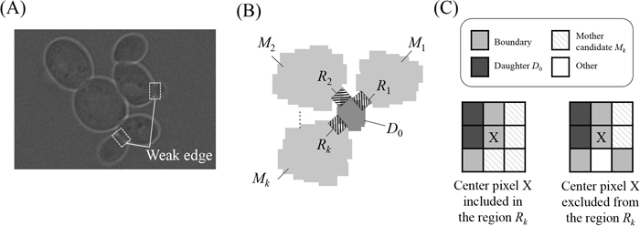
Daughter–mother association. (A) Raw image including a daughter–mother pair. Note that the boundaries between the daughter and mother cells in the white boxes are very weak. (B) Boundary region R_k (shaded region) between the daughter cell D₀ and its mother candidate M_k defined using the 3×3 mask shown in (C). (C) Center pixel X in the 3×3 mask included in or excluded from the boundary region R_k. Lower left panel, center pixel X included in R_k, whose 3×3 vicinity includes pixels belonging to D₀, M_k or boundaries; lower right panel, center pixel X excluded from R_k, whose 3×3 vicinity includes at least a pixel other than the one in D₀, M_k and boundaries.

Finally, the parent of each daughter was determined using B_k for each candidate. As in the tracking process, the simplest way to determine the mother of a daughter D₀ was to find the candidate M_k whose B_k was the minimum of all the candidates. However, because such a simple strategy increased identification errors, the annealing technique was utilized again. The parent cell was determined for each daughter cell whose minimum B_k was less than a prescribed threshold, and the threshold was gradually increased by a prescribed step size to identify the parents of the remainder of the daughter cells.

Manual correction for possible errors

After applying cell region extraction, cell tracking, and the daughter–mother cell association step to each frame of a set of time-lapse images, all the required properties of each cell were identified, including its area, perimeter, center of gravity, correspondence to a cell in the previous frame, and mother cell. These properties were stored for use in fluorescence analysis. However, several kinds of errors may occur during cell region extraction, the tracking step, and/or the daughter–mother association step, which can result in the assignment of erroneous properties to each cell. These errors were corrected manually.

For example, errors in the cell extraction process include cell over- and under-extraction and erroneous cell fragmentation or concatenation (Fig. 4A). These errors were manually corrected using a mouse-driven painting tool in our system. Erroneous association between cells was another type of error (Fig. 4B), which was corrected by directly editing the corresponding property (the corresponding cell in the previous frame or mother cell).

Fig. 4.

Examples of errors in the software system. (A) Error in cell region extraction and its manual correction. Upper panel, error in the cell extraction step, where the cell in the red circle fragments; lower panel, manual error correction using the painting tool. (B) Error in cell association between frames due to large motion. Upper left panel, the target cell for cell association; upper right panel, without manual correction. The corresponding cell is not identified in the next frame; lower right panel, manual correction that associates the target cell with the one in the red circle in the next frame. (C) Error propagation between frames. Red cells represent the progeny of cell #2. A daughter–mother association error in the 51st frame propagates to successive frames, which produces erroneous identifications of the progeny shown in the ellipse in the 85th frame. Manual correction of the error once in the 51st frame prevents all successive errors, leading to correct identifications in the 85th frame.

Figure 4C shows the propagation of an error between frames, where progeny of cell #2 are shown in red. The error in the daughter-mother association in the 51st frame affects successive daughter–mother associations, which produces an erroneous identification of the progeny unless a manual correction is performed in the 51st frame. Making one manual correction once in the 51st frame can prevent error propagation in successive frames.

Fluorescence analysis and generation of dendrogram

Because each cell was tracked over numerous frames and each and every daughter–mother association was identified, fluorescence analysis could be performed automatically by evaluating the fluorescence intensities for each cell using the pixel intensity in each cell region on each fluorescence image.

The result was recorded in an Excel file, similar to manual input, and the tree diagram was completed (Fig. 5). Differently colored circles are present on each branch because these cells were numbered manually in the order of birth, but in the automatic analysis system they were not numbered until the cell size exceeded a certain value. The expression level of cell region i is indicated by the evaluation value F_i. When ECFP was used, the fluorescence luminance was Y_i, the background fluorescence intensity was Y_bg, and the maximum luminance value was Y_max (arbitrary). Likewise, when mCherry was used, the fluorescence luminance was C_i, the background fluorescence intensity was C_bg, and the maximum luminance value was C_max (user-specified). Using this information, F_i is defined as   

$${\mathrm{F}}_{\mathrm{i}}=\left(\left({\mathrm{Y}}_{\mathrm{i}}-{\mathrm{Y}}_{\mathrm{b}\mathrm{g}}\right)/{\mathrm{Y}}_{\mathrm{m}\mathrm{a}\mathrm{x}}\right)/\left(\left({\mathrm{C}}_{\mathrm{i}}-{\mathrm{C}}_{\mathrm{b}\mathrm{g}}\right)/{\mathrm{C}}_{\mathrm{m}\mathrm{a}\mathrm{x}}\right).$$

Figure 5 shows an example of the dendrograms obtained after full manual analysis (upper) and by the software system with manual error correction (lower). Some branches differed at the top and bottom of the dendrograms, although we were able to output almost the same tree diagram. The difference in branching was due to cell numbering, but otherwise there was no essential difference between the dendrograms.

Fig. 5.

Dendrogram generation. Upper panel, the dendrogram obtained after full manual analysis; lower panel, the dendrogram obtained using the software with manual error correction. Circles on the vertical lines indicate identical cells in different frames, and branching indicates cell division. The ECFP signal is shown in green, and the EYFP signal in yellow. Cells that were no longer tracked or dead are shown as gray circles. The daughter–mother relationships of cells that divided from those in the first frame are set manually and shown as blue circles to distinguish them from those identified using the analysis method in Fig. 3.

Experimental results

Software-based computer-aided analysis was performed using the same data as used for manual analysis (101 bright-field images, 11 fluorescence images, 400 min tracking time) (Fig. 6). In a cell extraction, the system took 2 min to identify a total of 1,708 cells in each frame, and 15 min to identify and correct the three split errors. One reason for the division error was that high-intensity nuclei were regarded as cell boundaries. In cell tracking, an identical cell appearing in two consecutive frames was identified 1,650 times and daughter–mother relationships were identified 56 times, and these analyses took 30 sec. It took 30 min to identify and correct one pair of mistakes of an identical cell appearing in two consecutive frames and four pairs of mistakes in daughter–mother cell associations. Daughter–mother mistakes occurred frequently when the outline of the daughter cells was blurred in the bright field. Finally, it took 3 min to output the phylogenetic tree. The total analysis time was about 50 min.

Fig. 6.

Manual and automatic analysis times. Each step is displayed in a gray column and arranged in the order of analysis.

CONCLUSION

This study reports new software that greatly reduces the analysis time for time-lapse cell images of Saccharomyces cerevisiae. The software enables screening of silencing-related factors in S. cerevisiae and will contribute to the identification of genes affected by the heterochromatic region changes that occur between mother cells and daughter cells across generations.

ACKNOWLEDGMENTS

We thank Kohei Watarai and Hiroyuki Yoshimura for assisting in the development of the software. This study was supported by a grant from the Life Science Innovation Center (University of Fukui).

REFERENCES

•  Buzzetti,  E.,  Pinzani,  M., and  Tsochatzis,  E. A. (2016) The multiple-hit pathogenesis of non-alcoholic fatty liver disease (NAFLD). Metabolism 65, 1038–1048.
•  Hashimoto,  M.,  Nozoe,  T.,  Nakaoka,  H.,  Okura,  R.,  Akiyoshi,  S.,  Kaneko,  K.,  Kussell,  E., and  Wakamoto,  Y. (2016) Noise-driven growth rate gain in clonal cellular populations. Proc. Natl. Acad. Sci. USA 113, 3251–3256.
•  Hirano,  K.,  Yoshida,  T., and  Sakai,  Y. (2003) Edge enhancement and interpolation technique based on electric circuit simulation and its application to image segmentation. Electron. Comm. Jpn. 3 86, 22–33.
•  Kitada,  T.,  Kuryan,  B. G.,  Tran,  N. N. H.,  Song,  C.,  Xue,  Y.,  Carey,  M., and  Grunstein,  M. (2012) Mechanism for epigenetic variegation of gene expression at yeast telomeric heterochromatin. Genes Dev. 26, 2443–2455.
•  Kvarnström,  M.,  Logg,  K.,  Diez,  A.,  Bodvard,  K., and  Käll,  M. (2008) Image analysis algorithms for cell contour recognition in budding yeast. Opt. Express 16, 12943–12957.
•  Li,  K.,  Miller,  E. D.,  Chen,  M.,  Kanade,  T.,  Weiss,  L. E., and  Campbell,  P. G. (2008) Cell population tracking and lineage construction with spatiotemporal context. Med. Image Anal. 12, 546–566.
•  Mano,  Y.,  Kobayashi,  T. J.,  Nakayama,  J.,  Uchida,  H., and  Oki,  M. (2013) Single cell visualization of yeast gene expression shows correlation of epigenetic switching between multiple heterochromatic regions through multiple generations. PLoS Biol. 11, e1001601.
•  Meijering,  E.,  Dzyubachyk,  O., and  Smal,  I. (2012) Methods for cell and particle tracking. Methods Enzymol. 504, 183–200.
•  Meng,  X.-M.,  Nikolic-Paterson,  D. J., and  Lan,  H. Y. (2016) TGF-β: the master regulator of fibrosis. Nat. Rev. Nephrol. 12, 325–338.
•  Najman,  L., and  Schmitt,  M. (1994) Watershed of a continuous funtion. Signal Processing 38, 99–112.
•  Osborne,  E. A.,  Hiraoka,  Y., and  Rine,  J. (2011) Symmetry, asymmetry, and kinetics of silencing establishment in Saccharomyces cerevisiae revealed by single-cell optical assays. Proc. Natl. Acad. Sci. USA 108, 1209–1216.
•  Shen,  H.,  Tauzin,  L. J.,  Baiyasi,  R.,  Wang,  W.,  Moringo,  N.,  Shuang,  B., and  Landes,  C. F. (2017) Single particle tracking: from theory to biophysical applications. Chem. Rev. 117, 7331–7376.
•  Tsai,  H.-F.,  Gajda,  J.,  Sloan,  T. F. W.,  Rares,  A., and  Shen,  A. Q. (2019) Usiigaci: Instance-aware cell tracking in stain-free phase contrast microscopy enabled by machine learning. Softwarex 9, 230–237.
•  Tsuchida,  T., and  Friedman,  S. L. (2017) Mechanisms of hepatic stellate cell activation. Nat. Rev. Gastroenterol. Hepatol. 14, 397–411.
•  Van Valen,  D. A.,  Kudo,  T.,  Lane,  K. M.,  Macklin,  D. N.,  Quach,  N. T.,  DeFelice,  M. M.,  Maayan,  I.,  Tanouchi,  Y.,  Ashley,  E. A., and  Covert,  M. W. (2016) Deep learning automates the quantitative analysis of individual cells in live-cell imaging experiments. PLoS Comput. Biol. 12, e1005177.
•  Versari,  C.,  Stoma,  S.,  Batmanov,  K.,  Llamosi,  A.,  Mroz,  F.,  Kaczmarek,  A.,  Deyell,  M.,  Lhoussaine,  C.,  Hersen,  P., and  Batt,  G. (2017) Long-term tracking of budding yeast cells in brightfield microscopy: CellStar and the evaluation platform. J. R. Soc. Interface 14, 20160705.
•  Wang,  Q.,  Niemi,  J.,  Tan,  C.-M.,  You,  L., and  West,  M. (2010) Image segmentation and dynamic lineage analysis in single-cell fluorescence microscopy. Cytometry A 77, 101–110.
•  Winter,  M.,  Wait,  E.,  Roysam,  B.,  Goderie,  S. K.,  Ali,  R. A. N.,  Kokovay,  E.,  Temple,  S., and  Cohen,  A. R. (2011) Vertebrate neural stem cell segmentation, tracking and lineaging with validation and editing. Nat. Protoc. 6, 1942–1952.
•  Winter,  M. R.,  Liu,  M.,  Monteleone,  D.,  Melunis,  J.,  Hershberg,  U.,  Goderie,  S. K.,  Temple,  S., and  Cohen,  A. R. (2015) Computational image analysis reveals intrinsic multigenerational differences between anterior and posterior cerebral cortex neural progenitor cells. Stem Cell Reports 5, 609–620.