Consumer panic buying: Understanding the behavioral and psychological aspects

Abstract

Panic buying is a consumer behavior caused by negative emotions and social influences after a disaster. This study identifies (1) how panic buying occurs over time and (2) who panic buys. Based on the theoretical background of the behavioral and emotional nature of panic buyers, we conducted empirical segmentation to integrate behavioral and psychological data. This study focuses on Japanese consumer packaged goods during the COVID-19 outbreak and finds that there are two waves of increased purchases related to the timing of government interventions between February and April 2020. One of the unique features of this study is combining individual purchase data with psychological factors such as anxiety for COVID-19 and impulsiveness for unplanned purchase measured by a questionnaire survey. Another one is allowing for heterogeneity among consumers in terms of demographic or psychographic characteristics. The results show that panic buying occurred for a limited segment of consumers, that is, consumers with more purchasing experience, including female with larger families hardly panic buy and rather stockpile a little more than usual.

1.  INTRODUCTION

Panic buying is a phenomenon often seen after a major disaster, such as an earthquake (Forbes, 2017; Hori & Iwamoto, 2014) or the SARS crisis (Cheng, 2004). During the COVID-19 pandemic, panic buying emptied store shelves around the world, and understanding this phenomenon has been the focus of recent research (Kirk & Rifkin, 2020; Loxton et al., 2020; Prentice, Chen, & Stantic, 2020; Yuen, Wang, Ma, & Li, 2020). When panic buying causes products to become scarce and prices to soar, consumer welfare is affected, and long-term relationships between firms and customers are destabilized. Thus, policymakers and marketers must heed the consumer and psychology research that has examined the mechanism of panic buying during the COVID-19 outbreak (Dholakia, 2020a; 2020b; Notebaert, 2020; Novemsky, 2020).

The Oxford English Dictionary defines panic buying as “the action of buying large quantities of a particular product or commodity due to sudden fears of a forthcoming shortage or price rise.” It has long been known that people exhibit panic responses after a disaster. According to Fritz and Marks (1954, p. 30), “the term ‘panic’ has been used quite widely to describe a wide variety of ‘irrational’ behavior of individuals exposed to danger situations.” Hall, Fieger, Prayag, and Dyason (2021, p. 2) states “panic buying is not necessarily caused by a supply deficit per se, although perceptions of a future deficit are significant, but by consumers’ heightened anxiety and fear.” It is a variant of stockpiling which is modeled as a rational, forward-looking behavior (Meyer & Assunção, 1990; Sun, 2005; Sun, Neslin, & Srinivasan, 2003). However, panic buying goes beyond rational stockpiling since (1) it is a response to a state of emergency, for example, a pandemic, natural disaster, or economic crisis; (2) purchases often exceed the optimal level required for the expected shortage; and (3) the panic is often laden with negative emotions, such as anxiety or fear. Hence, the term “stockpiling” has been used when it is considered to be a rational or adaptive response, while the term “panic buying” has been used when the behavior is excessive, irrational or emotional attempt (Lee, Wu, & Lee, 2021; Rajkumar & Arafat, 2021). Panic buying also differs from “hoarding disorder,” a term that is often used in pathological contexts, such as that of a compulsive disorder (Frost & Gross, 1993; Steketee & Frost, 2003). There are several reasons why consumers panic: (1) to alleviate anxiety, fear and to control their lives, (2) as a reaction to anticipated future scarcity, and (3) in response to the buying patterns of others, for example, after seeing empty shelves or to conform to the behaviors of friends or family members (Dholakia, 2020a, 2020b; Notebaert, 2020).

Although panic buying is a common phenomenon after disasters, it was a niche research area, and recent research mentioned that there are few psychological studies dealing with it (Bentall et al., 2021; Yuen et al., 2020). In contrast, as panic buying became a serious problem in many parts of the world due to the threat of COVID-19, there is an increase in empirical research addressing individual-level psychological factors related to panic buying. However, most of the studies are based on questionnaire surveys (e.g., Bentall et al., 2021; Chua, Yuen, Wang, & Wong, 2021; Islam et al., 2021; Kemp, Kennett‐Hensel, & Williams, 2014), and it is not clear to what extent psychological factors are reflected in actual purchasing behaviors. In this study, we uniquely attempt to understand both behavioral and psychological aspects by integrating different types of data at an individual level: actual purchase data and psychographics obtained from a survey. This allows us to explain the quantitative degree of panic buying by consumers (e.g., how much more they purchased, and in which product categories the extra purchases were) and the psychological factors behind it.

In addition, the limitations are that most studies have focused on a mere one-time panic buying opportunity. In the early stages of a pandemic, more consumers may panic buy. However, it is assumed that the degree of panic buying within individual consumers will change over time. To the best of our knowledge, little is known about how individuals change their behavior in multiple panic buying occasions. By analyzing this behavior, we can understand how consumers learn from their past experiences and make their next purchases.

This empirical study aims to identify: (1) how panic buying occurs over time; and (2) who panic buys. Specifically, it focuses on two waves of panic buying in Japan and structurally classifies consumers’ buying patterns at that time. We also evaluated the contribution of consumer demographics, psychographics, and media usage to the segments. In the analysis, we first measured the magnitude of the temporary purchase increases in 173 product categories of consumer packaged goods using scanner panel data. Next, for each of these categories, we evaluated the increase in purchase amounts compared to previously for each individual and conducted consumer segmentation. To collect psychographic data, we administered a questionnaire survey to the same respondents. This hybrid approach enabled us to integrate quantitative modeling with a psychological survey.

The remainder of this paper introduces evidence from Japan on the temporary purchase increases and reviews the literature related to consumer panic buying. We then detail the research framework, explain our data and models, and present the results. Finally, the discussion section concludes the paper with a discussion of the managerial implications of our findings.

2.  CONCEPTUAL DEVELOPMENT AND LITERATURE REVIEW

The relationship between the timing of government intervention and purchase increase: Evidence from Japan

In the early stages of the COVID-19 pandemic in Japan, temporary purchase increases of consumer packaged goods linked to government interventions were observed. We begin with a timeline of the spread of COVID-19 and the two main government interventions: the temporary closure of elementary and secondary schools and the first state of emergency. Figure 1 shows the number of COVID-19 infections from January 1 to May 31, 2020 (Ministry of Health, Labor & Welfare, 2020). The first infection was confirmed in Japan on January 16. Subsequently, with the increased awareness of the COVID-19 crisis, the government issued a temporary closure of elementary and secondary schools on February 27. As the number of infections continued to rise from the end of March, the government declared the first state of emergency in major cities, including Tokyo and Osaka, on April 7, after which the declaration was extended nationwide on April 16. Consequently, the number of infections gradually declined, and the first state of emergency was lifted on May 25.

Figure 1

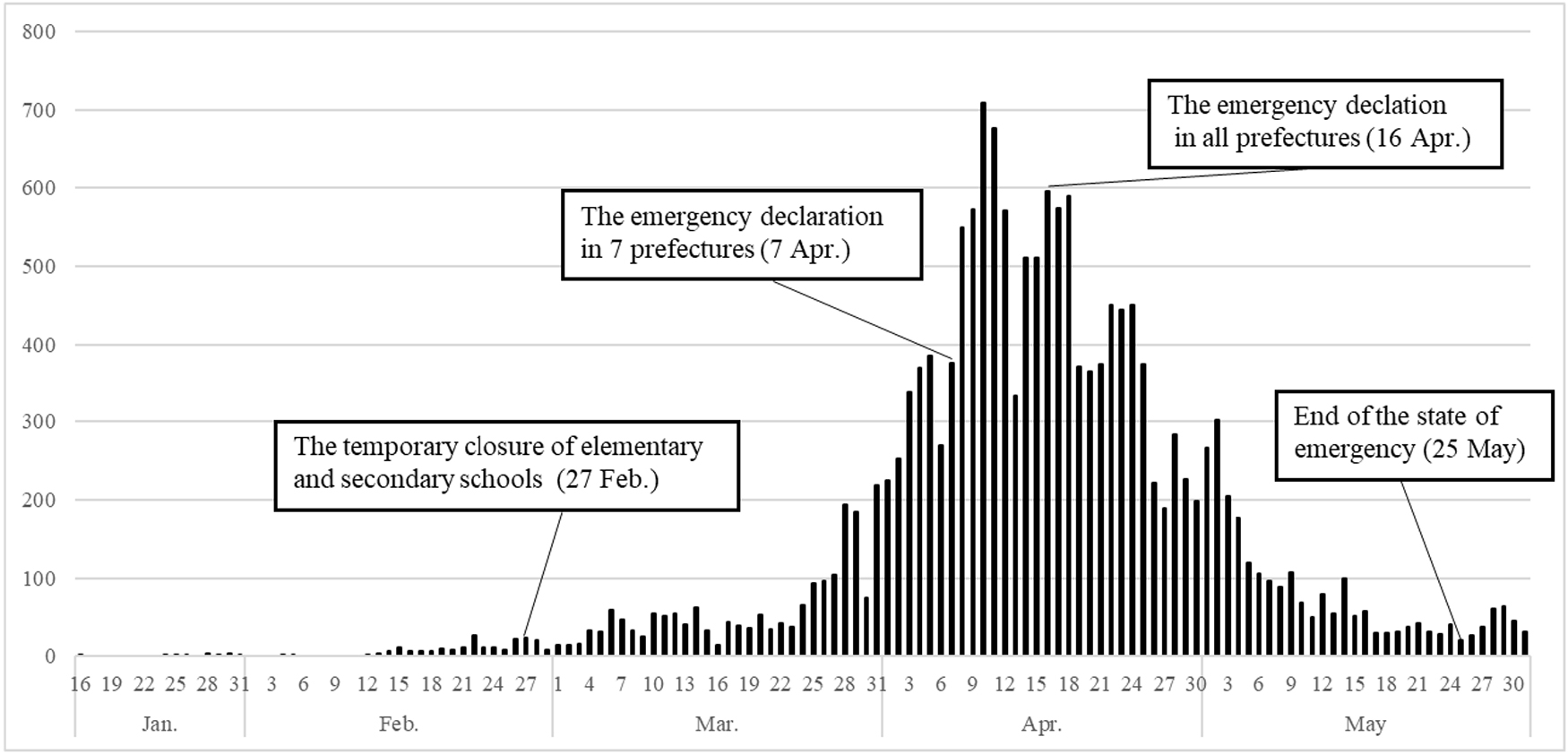
The number of COVID-19 infections in Japan.

Previous research indicates that government interventions can cause temporary purchase increases (e.g., Prentice et al., 2020), and our case in Japan confirms this as well. Figure 2 shows the time series of the year-on-year ratio (7-day moving average) of the purchase amount of consumer packaged goods, which was calculated using the Syndicated Consumer Index (SCI), Japan’s largest consumer individual-level scanner panel data¹⁾. The year-on-year purchase amount ratio was computed by dividing the purchase amount per panelist on each date in 2020 with that of 2019. Based on the data, the first wave of temporary increases occurred after the declaration of school closures. The second wave was also associated with the declaration of the first state of emergency. The second wave was different from the first, in that the purchase amount did not increase immediately after the declaration of the state of emergency. The declaration was anticipated and reported extensively on television news and other media before it was issued; hence, there was an increase approximately one week before the declaration. This study focuses on the two waves of temporary purchase increases in response to these government interventions.

Figure 2

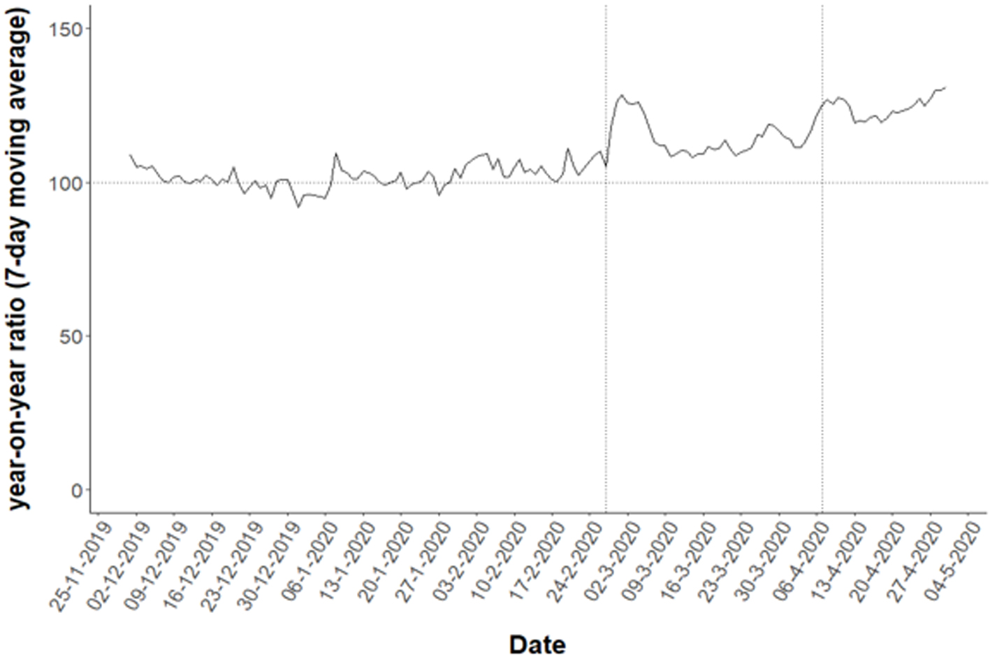
Time series of the year-on-year ratio (7-day moving average) of the purchase amount of consumer packaged goods. Note. The vertical line on the left represents the declaration of the school closure (February 27), and the vertical line on the right represents the declaration of a state of emergency in major cities (April 7).

Individual factors related to panic buying

Previous studies have highlighted several factors contributing to panic buying. Rajkumar and Arafat (2021) classified the factors into three categories: (1) disaster-related factors such as severity and duration of the event; (2) individual factors including psychological and informational factors; and (3) supply and demand related factors such as a limited supply of essentials. With regard to the first of these, we have already pointed out that government interventions in response to the severity of COVID-19 led to panic buying. On that basis, this study will focus on individual factors to understand the characteristics of panic buyers. Table 1 summarizes previous studies on the individual factors of panic buying.

Table 1 Literature on individual factors of panic buying

Paper	Factors related to panic buying					Data
		Negative emotions	Purchase characteristics	Social influence	Others
Cheng (2004)	Anxiety, Fear, Hopelessness, Distress	✓				Population-based survey
Gasink et al. (2009)	Worry about influenza	✓				Survey of clinic patients
Hori & Iwamoto (2014)	Demographics: larger number of family members, urban area, older age, homemaker wives				✓	Scanner panel data
Kemp et al. (2014)	Anxiety, Fear, Lack of control, Rumination	✓				Online survey
Khare et al. (2019)	Social media: number of tweets, Public warning of hurricane			✓		Tweet data
Naeem (2020)	Social media			✓		Telephonic interview
Yuen et al. (2020)	Perceived threat, Perceived scarcity, Fear of the unknown, Coping behavior, Social influence, Social trust	✓		✓		Systematic literature review
Bentall et al. (2021)	Demographics: male, number of children, income, Paranoia, Depression, Death anxiety, Cognitive reflection task, Personal risk	✓			✓	Online survey
Chua et al. (2021)	Perceived scarcity, Anticipation of regret, Online shopping frequency		✓		✓	Online survey
Islam et al. (2021)	Scarcity, Social media, Arousal, Urge to buy impulsively		✓	✓	✓	Online survey
Lee et al. (2021)	Risk perception, State anxiety, Trust in social media	✓		✓		Survey of students
This paper	Anxiety Psychographics: Impulsiveness, Price consciousness, Conformity, Feelings of guilt Media usage: TV news, mobile news, social media, EC Demographics	✓	✓	✓	✓	Single source data including scanner panel data, device log data and online survey

One of the most fundamental elements is that panic buying is accompanied by negative emotions, such as anxiety (Cheng, 2004; Kemp et al., 2014; Lee et al., 2021) and fear (Cheng, 2004; Kemp et al., 2014; Sterman & Dogan, 2015). After a natural disaster, these undesirable negative emotions can arise when an individual feels a lack of control of the situation (Kemp et al., 2014). Mawson (2005) categorized individual reactions to disasters as being triggered by anxiety when the perceived risk of physical danger is mild, and fear when it is severe. The present study deals with the period between February and April 2020, when the fear of the threat of COVID-19 was spreading among the Japanese public. Because few people were in a state of severe physical danger at that stage, our central focus is placed on anxiety. In our study, we explicitly use the terms “hoarding” and “panic buying” differently, defining panic buying as hoarding behavior conducted by consumers experiencing anxiety.

In terms of consumer purchase characteristics, panic buying is characterized by impulsive and unplanned consumer behavior (Dholakia, 2020a; Islam et al., 2021). Although impulsive buying has long been studied in consumer behavior research (e.g., Rook, 1987), panic buying is a variant of impulsive buying, in which consumers suddenly flock to stores instead of maintaining their regularly scheduled shopping. In such a situation, perceived scarcity (Chua et al., 2021; Islam et al., 2021; Sterman & Dogan, 2015; Yuen et al., 2020) and expectations of supply shortages (Yoon, Narasimhan, & Kim, 2018) cause consumers to buy things they do not really need; therefore, it is likely that panic buyers buy indiscriminately based on availability, rather than preference or price (Dholakia, 2020a).

Panic buying is also triggered by social influence. Panic buying is caused by being influenced by the actions of others, such as looking at empty shelves and listening to friends and family members (Dholakia, 2020b). The tendency to imitate or conform to the behavior of others is reflected in this behavior. Furthermore, several other studies have demonstrated the influence of the media. Naeem (2020) found that social media enhances social exchanges and develops social influences, thus increasing consumer panic buying. Naeem (2020) also implied that even though real-time information about COVID-19 on social media sites can encourage people to make smart decisions, it can also make them more anxious and lead to panic buying. Similarly, Islam et al. (2021) revealed that excessive social media use is related to panic buying during the crisis.

Research framework

Figure 3 illustrates the present study’s conceptual framework. As noted in the previous section, there was an association between the timing of government policy interventions and the temporary purchase increases of consumer packaged goods. In particular, we focused on the two waves of purchase increases in Japan in response to the two policy interventions. However, even if there was an increase in purchases at the aggregate level of the market, each consumer’s actions would be different; therefore, we took a segmentation approach to understand the heterogeneity among consumers during this time.

Figure 3

Conceptual framework.

We first identified temporarily hoarded product categories. Here, we evaluated the purchase increases in response to the two policy interventions in an aggregate time series for each product category. Second, we captured consumer hoarding at an individual level; if an individual made more purchases than in the previous year, the individual is considered as a hoarder. Using the amount of an individual’s hoarding, we then conducted consumer segmentation. After the segmentation, we evaluated the members of the segment by demographics, psychographics, and media usage. This is discussed in detail in the next section.

3.  METHODS

Identification of temporarily hoarded product categories

As previously mentioned, as far as the total value of consumer packaged goods, there were two temporary purchase increase waves related to government interventions. However, those increases did not necessarily occur in each product category. Hence, we first identified the product categories that consumer temporarily hoarded, using scanner panel data (SCI); the sample size used in this analysis is 38,213, the same as in Figure 2. We obtained data for 173 categories of consumer packaged goods for the time series of the year-on-year ratio (7-day moving average) of purchase amounts from December 1, 2019, to April 28, 2020. Consumer packaged goods include groceries, beverages, daily necessities, cosmetics and drugs.

To identify the temporary purchase increases in each category, we focused on the waveforms of the time series. As shown in Figure 4, we set two conditions using the peak of the wave and the mean before / after government interventions. The first condition is the degree of increase compared to normal times. Specifically, we examined the degree of increase within short term after the government intervention compared to the mean value before the intervention. The second is to verify whether the increase is temporary or not. Specifically, we examined the extent to which purchases returned to normal using the mean value during sufficiently long term after the intervention.

Figure 4

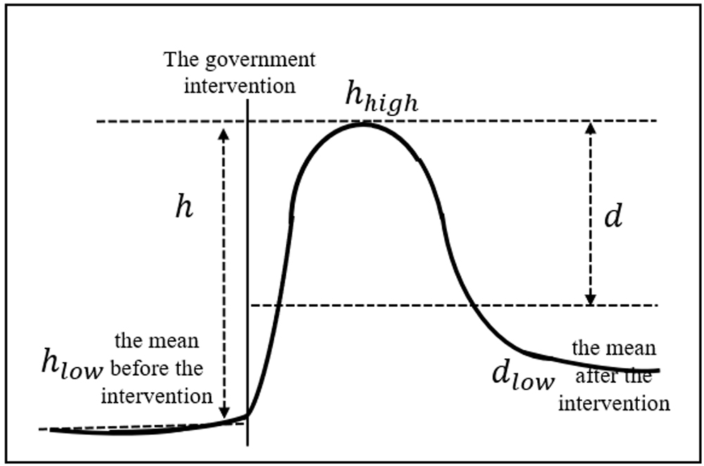
Parameters for the waveform.

This study attempts to identify temporary increase from actual purchase data, but to the best of our knowledge, there has been little research on panic buying from this perspective. Therefore, with respect to the identification of the waveform, we drew inspiration from Goldenberg, Libai, and Muller (2002) in the adjacent marketing field. Goldenberg et al. (2002) parameterized the peak and trough of the waveform and identified the shape of the waveform in an a priori way²⁾. For this operation, the variables (1) the peak of the waveform and (2) the return depth from the peak were used³⁾. This also works well for us to capture temporary purchase increase from the waveform. However, it cannot simply be applied, so we operate it as described below.

First, we measured the peak and baseline in the waveform to capture the purchase increase (not necessarily temporary) in each category (see also Figure 4). Let h_low be the baseline, measured as the mean value from December 1, 2019 to February 26, 2020 (the day before the declaration of the school closures). Let h_high be the peak of the wave, measured as the maximum value within two weeks of the government interventions. $h_{\mathit{high}}^{\left(1\right)}$ is defined as the maximum value during the two weeks from February 27 (the declaration of school closures) to March 11, and $h_{\mathit{high}}^{\left(2\right)}$ is defined as the maximum value during the two weeks from April 1 (a week before the declaration of a state of emergency) to April 14. We define the maximum value of the waveform as the peak, but the maximum value is susceptible to an outlier. In order to reduce the impact of an outlier, we use a 7-day moving average as a time series indicator. This operation removes random variations that appear as coarseness in a plot of raw time series data. In addition, we set the measurement period of h_high to two weeks because the peak and trough of purchase increases in total of all categories occur in about two weeks (see also Figure 2). Furthermore, since the periods during which the peaks and troughs occurred are similar for the first and second waves, the periods for $h_{\mathit{high}}^{\left(1\right)}$ and $h_{\mathit{high}}^{\left(2\right)}$ are defined as equal to two weeks. In the specification of the period of $h_{\mathit{high}}^{\left(2\right)}$, we set the starting point a week before the declaration of the state of emergency because there was a purchase increase before the declaration was issued as it was expected in advance and widely reported in the media. Using these values, the increase in purchase amount h is defined as $h^{\left(1\right)}=h_{\mathit{high}}^{\left(1\right)}-h_{\mathit{low}}$ in the first wave and $h^{\left(2\right)}=h_{\mathit{high}}^{\left(2\right)}-h_{\mathit{low}}$ in the second wave.

Next, we confirmed whether the purchase increases were temporary. Let d_low be the return value of the waveform measured as the mean value during the four weeks after the government intervention. We set a time frame of four weeks, which is long enough to take into account the intervention interval. $d_{\mathit{low}}^{\left(1\right)}$ is defined as the mean value from February 27 to March 26, and $d_{\mathit{low}}^{\left(2\right)}$ is defined as the mean value from April 1 to April 28. We expressed the return value of the waveform d as $d^{\left(1\right)}=h_{\mathit{high}}^{\left(1\right)}-d_{\mathit{low}}^{\left(1\right)}$ for the first wave and $d^{\left(2\right)}=h_{\mathit{high}}^{\left(2\right)}-d_{\mathit{low}}^{\left(2\right)}$ for the second wave. Table 2 summarizes the variable definitions discussed above.

Table 2 Summary of variable definitions

hlow	Baseline measured as the mean value from December 1, 2019 to February 26, 2020 (the day before the declaration of the school closures)
hhigh	The peak of the wave measured as the maximum value within two weeks of the government intervention
$h_{\mathit{high}}^{\left(1\right)}$	The maximum value during the two weeks from February 27 (the declaration of school closures) to March 11
$h_{\mathit{high}}^{\left(2\right)}$	The maximum value during the two weeks from April 1 (a week before the declaration of a state of emergency) to April 14
h(1)	$h^{\left(1\right)}=h_{\mathit{high}}^{\left(1\right)}-h_{\mathit{low}}$
h(2)	$h^{\left(2\right)}=h_{\mathit{high}}^{\left(2\right)}-h_{\mathit{low}}$
dlow	The return value of the waveform measured as the mean value during the four weeks after the government intervention
$d_{\mathit{low}}^{\left(1\right)}$	The mean value from February 27 to March 26
$d_{\mathit{low}}^{\left(2\right)}$	The mean value from April 1 to April 28
d(1)	$d^{\left(1\right)}=h_{\mathit{high}}^{\left(1\right)}-d_{\mathit{low}}^{\left(1\right)}$
d(2)	$d^{\left(2\right)}=h_{\mathit{high}}^{\left(2\right)}-d_{\mathit{low}}^{\left(2\right)}$

Note that the reason we defined the d conditions in this way is to remove the effect of a sustained demand increase. For example, in some product categories, the purchase increases were not temporary but continuous due to the influence of people staying at home. In this case, the waveform had a narrower peak and trough, and the value of d was smaller. Such product categories are regarded, in this study, as not temporary purchase increases related to panic buying. Added to this, we treat d_low as the mean value, not the minimum value. This is because we need to exclude the pattern of a momentarily drop and then continuing to rise again. Since the minimum value does not exclude this pattern, the mean value is appropriate.

We first calculated h and d for the total value of consumer packaged goods for the two observed waves. We then calculated these values for each category and identified the categories with temporary purchase increases in which both h and d were greater than the total value⁴⁾. 52 categories in the first wave and 63 categories in the second wave were extracted (see Appendix Tables A.1 and A.2 for further details)⁵⁾. We used these temporarily hoarded product categories for the subsequent analysis.

Data

Multiple data tied at individual levels are used for the segmentation analysis, comprising purchase history of scanner panel data, demographics, psychographics collected via a survey, and device log data from television and mobile devices. These data were collected by INTAGE Inc., a Japanese marketing research company. The purchase history and device log data are representative panel data that have been utilized in the marketing by many companies in Japan. We further conducted a questionnaire survey on the panelists to obtain the psychographics. Ultimately, 968 respondents are included in this study.

Purchase History. For the product categories where hoarding occurred, we indexed the amount of hoarding compared to normal at the individual level. q_i1 represents the purchase amount (yen) of respondent i for the corresponding categories for two weeks during the first wave (from February 27 to March 11, 2020). q_i2 is the purchase amount for the corresponding categories for two weeks during the second wave (from April 1 to 14, 2020). Since q_i1 and q_i2 are defined by aggregating multiple categories, rather than by individual categories, the effect of purchase intervals for individual products is eliminated. Next, $\stackrel{-}{q_{i1}}$ represents the average purchase amount per two weeks for the corresponding categories during the first wave (see Appendix Table A.1) in the past year (from February 1, 2019, to January 31, 2020). Similarly, $\stackrel{-}{q_{i2}}$ is the average purchase amount per two weeks in the corresponding categories during the second wave (see Appendix Table A.2) in the past year (from February 1, 2019, to January 31, 2020). Using these, we define y_i1 and y_i2 (consumer hoarding indexes) as the extent to which consumers hoarded more than usual.   

$$y_{i1}=\log \left(q_{i1}\right)-\log \left(\stackrel{-}{q_{i1}}\right)\text{,}{y}_{i2}=\log \left(q_{i2}\right)-\log \left(\stackrel{-}{q_{i2}}\right)$$(1)

Note that $\stackrel{-}{q_{i1}}$ and $\stackrel{-}{q_{i2}}$ are defined as the values of the annual average per two weeks, not the values of the same period in the previous year of q_i1 and q_i2. Unlike the aforementioned analysis of aggregated time series data, in the analysis of purchase amounts at the individual level, the magnitude of intra-individual variability becomes larger, if $\stackrel{-}{q_{i1}}$ and $\stackrel{-}{q_{i2}}$ are just two weeks of data. Hence, to avoid the noise, we use the annual average per two weeks.

Table 3 presents the summary statistics for these variables. Figure 5 shows the plots of the consumer hoarding indexes y_i1 and y_i2, which take positive values when consumption increased compared to the average purchase amount in the past year and negative values when it decreased. The correlation coefficient is 0.124, suggesting that across the sample population, the first and second waves of hoarding did not necessarily occur among the same individuals.

Table 3 Summary statistics of the variables for purchase amounts

	mean	sd	min	max
qi1	3050.1	3132.9	82.0	37938.0
$\stackrel{-}{q_{\mathrm{i}1}}$	2304.8	1695.9	51.1	11838.1
qi2	2922.0	2977.8	59.0	33016.0
$\stackrel{-}{q_{\mathrm{i}2}}$	2252.8	1728.7	95.9	15180.4
yi1	0.082	0.863	−3.100	2.888
yi2	0.054	0.280	−2.774	3.332

Figure 5

Plot of consumer hoarding index in first and second waves.

Psychographics. The survey data were collected from April 23 to 27, 2020. As shown in Table 4, we measured the psychographic constructs using multiple items with a 7-point Likert scale ranging from 1 (fully disagree) to 7 (fully agree). The first construct is perceived anxiety of COVID-19. Anxiety is measured using three items, following Maheswaran and Meyers-Levy (1990) and Winterich and Haws (2011). The second construct is impulsiveness, which represents consumer propensity for impulsive and unplanned purchasing. Impulsiveness was tested using two items from Ailawadi, Neslin, and Gedenk (2001). The third construct is price-consciousness, representing consumers’ perceptions of price and we used three items as defined by Ailawadi et al. (2001) to test for it. If panic buying is a price-independent hoarding behavior (Dholakia, 2020a), then this construct is expected to have a negative effect on such behavior. The fourth is conformity, which represents social relationships and is defined as how easily one’s choices depend on others. We borrowed two items from Mehrabian and Stefl (1995). The last construct is guilt, which expresses how much guilt consumers feel when they make a purchase that cannot be logically justified. We borrowed three items from Mishra and Mishra (2011) for guilt.

Table 4 Variable measurements for psychographics

		Loading	Cronbach’s alpha	Composite reliability	AVE
Anxiety	I feel tense about the COVID-19 outbreak.	0.888	0.866	0.870	0.692
	I feel anxious about the COVID-19 outbreak.	0.810
	I feel fearful about the COVID-19 outbreak.	0.804
Impulsiveness	I often make an unplanned purchase when the urge strikes me.	0.921	0.805	0.822	0.702
	I often find myself buying products on impulse in the grocery store.	0.732
Price consciousness	I compare the prices of at least a few brands before I choose one.	0.829	0.819	0.824	0.612
	I find myself checking the prices even for small items.	0.787
	It is important to get the best price for the products I buy.	0.722
Conformity	I often rely and act upon the advice of others.	0.814	0.764	0.764	0.618
	I tend to rely on others when I have to make an important decision quickly.	0.760
Feelings of guilt	I feel guilty when I make impulse purchases	0.796	0.727	0.734	0.512
	I regret when I make purchases that I am unable to logically justify.	0.718
	I feel guilty when considering luxurious products and services that are pleasurable but not necessary	0.562

Correlation matrix	1	2	3	4	5
1. Anxiety	0.832
2. Impulsiveness	0.074	0.838
3. Price consciousness	0.267	−0.242	0.783
4. Conformity	0.161	0.298	0.121	0.786
5. Feelings of guilt	0.243	−0.220	0.449	0.243	0.716

Note. Diagonal values of the correlation matrix represent the square root of average variance extracted (AVE) values. All other values represent the correlation coefficients.

Confirmatory factor analysis (Table 4) demonstrated that the goodness-of-fit index (GFI) = 0.976, comparative fit index (CFI) = 0.979, and the root mean squared error of approximation (RMSEA) = 0.043. Cronbach’s alpha values and composite reliability (CR) values are above the cut-off criterion of 0.7 (Bagozzi & Yi, 1988; Hair, Black, Babin, & Anderson, 2010). For convergent validity, average variance extracted (AVE) values of all constructs are greater than 0.5. For discriminant validity, evidence is present when the square root of the AVE for each construct exceeds the corresponding correlations between that and any other construct (Fornell & Larcker, 1981). Our results met this condition.

Demographics. We used the six demographics of gender, age, number of family members, number of children, household income (ten million yen), and education level. Gender is expressed as a dummy variable, where 1 represents male. Other demographics are expressed as continuous variables. The number of children is defined as the number of children under the age of 14 in a household. Education level is quantified by the number of years of education after elementary school.

Device Log Data from Television and Mobile Devices. Log data of television viewing and mobile usage were used in this study. The television data were automatically coded to identify which program each respondent watched at a certain time; we created television news and talk show variables to define their average daily usage (minutes). The mobile data were also automatically coded to identify which app each respondent used on their smartphones; we created social networking services (SNS), mobile news, e-commerce (EC), and healthcare variables to define average daily usage (minutes). These app categories were identified based on information from the Google Play Store. The observed period was from February 27 to April 14, 2020, corresponding to the period between the two policy interventions (from the declaration of the school closure to one week after the state of emergency). This period also corresponded to the period of the purchase variables. Table 5 shows the summary statistics of the samples.

Table 5 Summary statistics

	mean	sd
Gender (male = 1)	0.42	0.49
Age	47.96	11.82
Number of family members	2.83	1.22
Number of children	0.45	0.78
Income	0.61	0.28
Education	14.42	1.77
SNS	10.36	22.22
Mobile news	23.63	41.08
EC	3.70	10.02
Healthcare	0.86	3.16
TV news	37.84	39.33
TV talk shows	43.05	50.39

Model

We used the Gaussian mixture model (McLachlan & Peel, 2000) to segment consumers using two indicators of consumer hoarding index, y_i1 and y_i2. The model can be expressed as follows:   

$$f\left({\mathit{y}}_i\right)=\sum _{k=1}^K{\pi }_k{f}_k\left({\mathit{y}}_i|{\mathit{\mu }}_k,{\mathbf{\Sigma }}_k\right)$$(2)

y_i = (y_i1, y_i2)' is the vector of response variables for respondent i. f_k(y_i|μ_k, Σ_k) is the kth component density for y_i. Each component is assumed to have a Gaussian distribution N(μ_k, Σ_k); μ_k is a mean vector, and Σ_k represents the covariance matrix. π_k is a mixing coefficient, where 0 ≤ π_k ≤ 1 and Σ_kπ_k = 1. We used the EM algorithm to estimate the model (Fraley & Raftery, 1998; McLachlan & Peel, 2000).

After identifying the segments, we used a multinomial logit model to descriptively interpret the characteristics of the segments.   

$$\mathit{Pr}\left(s_i=k|{\mathit{x}}_i\right)=\frac{exp\left({\mathit{x}}_i\prime {\mathit{\beta }}_k\right)}{{\sum }_{k=1}^{K}exp\left({\mathit{x}}_i\prime {\mathit{\beta }}_k\right)}$$(3)

where s_i is the indicator of respondent i’s segment; x_i is a vector of demographics, psychographics, and media use variables for respondent i; and β_k is the parameter vector. As a base segment for the multinomial logit model, which is the alternative normalized to have coefficients equal to zero (Cameron & Trivedi, 2005), we chose Segment 1, which has the largest number of respondents and set β₁ = 0.

4.  RESULTS

To determine the number of segments, we first estimated the model by varying the number of segments from one to seven. The EM algorithm used for the estimation is sensitive to the initial values of the parameters (Masyn, 2013). Thus, to reduce the likelihood of convergence to local maxima, we estimated the model with 50 random sets of starting parameters and adopted the minimum log-likelihood model as the best model for each number of segment models. Next, we calculated the Akaike Information Criterion (AIC), the Bayesian Information Criterion (BIC) (Schwarz, 1978) and the Consistent AIC (CAIC) (Bozdogan, 1987) as shown in Table 6. We obtained the minimum BIC and CAIC value for the five-segment model, while the AIC value was minimized in the six-segment model. Among the three criteria, the penalization is least strong in the AIC, stronger in the BIC, and strongest in the CAIC. It is known that there is a possibility that AIC overestimates the number of segments in a segmentation using a mixture model (Collins & Lanza, 2009). Therefore, we adopted the five-segment model as the best model based on the results supported by the two information criteria, BIC and CAIC.

Table 6 Log-likelihood statistics for model selection

	LL	AIC	BIC	CAIC
1-Segment	−2501.3	5012.5	5036.9	5041.9
2-Segment	−2395.4	4812.8	4866.5	4877.5
3-Segment	−2353.8	4741.6	4824.5	4841.5
4-Segment	−2317.0	4679.9	4792.0	4815.0
5-Segment	−2287.8	4633.6	4775.0	4804.0
6-Segment	−2274.1	4618.2	4788.9	4823.9
7-Segment	−2268.2	4618.3	4818.2	4859.2

Our segmentation results are clear and correspond to the magnitude of hoarding during the first and second waves. Table 7 shows the profile of purchasing for each segment. Table 8 details the demographics, psychographics, and media use variable coefficients, representing the impact of each variable on segment membership. Note that Segment 1 is the base segment, and the parameters are fixed at 0.

Table 7 Profile of purchasing

		Number of samples		Mean		Mean (a)		Mean (b)		a/b (%)
		n	%	yi1	yi2	qi1	qi2	$\stackrel{-}{q_{\mathrm{i}1}}$	$\stackrel{-}{q_{\mathrm{i}2}}$	1st	2nd
1	Experienced shoppers	379	39.2%	0.216	0.145	3534	3166	2750	2646	129%	120%
2	Inactive shoppers	235	24.3%	−1.000	−0.074	883	2540	2146	2065	41%	123%
3	Weak panic buyers	153	15.8%	0.417	−1.020	3484	919	2129	2184	164%	42%
4	Rational shoppers	145	15.0%	0.530	0.945	3624	5060	2000	1944	181%	260%
5	Strong panic buyers	56	5.8%	1.630	0.591	6197	2818	1228	1370	505%	206%

Table 8 Parameter estimates of the segment membership coefficients

	Variables	Inactive shoppers		Weak panic buyers		Rational shoppers		Strong panic buyers
		coef.	s.e.	coef.	s.e.	coef.	s.e.	coef.	s.e.
Demographics	Constant	1.789	0.845**	−0.506	1.003	1.104	0.990	−4.514	1.586***
	Gender (male = 1)	0.538	0.184***	0.380	0.212*	0.345	0.218	1.430	0.325***
	Age	−0.009	0.008	0.007	0.010	−0.017	0.010*	0.015	0.016
	Number of family members	−0.271	0.097***	−0.364	0.115***	−0.217	0.117*	−0.052	0.170
	Number of children	0.044	0.152	0.231	0.178	0.254	0.167	0.564	0.241**
	Income	0.386	0.332	0.348	0.386	0.645	0.393	−0.195	0.591
	Education	−0.114	0.050**	−0.023	0.059	−0.093	0.059	0.065	0.090
Psychographics	Anxiety	0.085	0.097	0.225	0.115*	0.006	0.111	0.489	0.183***
	Impulsiveness	0.029	0.096	0.200	0.110*	−0.228	0.109**	0.456	0.173***
	Price consciousness	0.016	0.098	0.110	0.115	0.255	0.116**	0.236	0.182
	Conformity	−0.174	0.104*	−0.134	0.120	−0.240	0.122**	−0.084	0.182
	Feelings of guilt	0.081	0.103	0.203	0.121*	−0.094	0.116	−0.065	0.179
Media use	SNS	0.008	0.004**	0.006	0.005	−0.006	0.006	0.007	0.007
	Mobile news	0.001	0.002	0.000	0.003	0.005	0.002**	0.007	0.003**
	EC	−0.013	0.010	−0.010	0.010	−0.009	0.011	−0.053	0.031*
	Healthcare	−0.013	0.028	0.007	0.028	−0.016	0.034	−0.030	0.055
	TV news	0.001	0.003	0.000	0.003	−0.001	0.003	0.000	0.004
	TV talk shows	0.000	0.002	0.001	0.002	0.001	0.002	−0.001	0.004

Note. *** p < .01, ** p < .05, * p < .10.

Segment 1, which has the highest composition ratio (39.2%), includes typical household shoppers who often purchase daily consumer goods. Because the mean values of $\stackrel{-}{q_{i1}}$, $\stackrel{-}{q_{i2}}$ in this segment, which represent the average purchase amounts under a normal condition (not under a pandemic), are higher than other segments, we label this segment experienced shoppers. In Table 8, the coefficients of gender in segments 2–4 are positive and include more males, indicating that, conversely, this base segment includes more females. Similarly, segment 1 has the larger number of family members. This segment, which is a standard household with a large number of family members and female shoppers, increased purchases to 129% during the 1st wave and 120% during the 2nd wave compared to normal (Table 7).

It is important to note that these consumers only stockpiled small amounts within the bounds of common sense. This study suggests that panic buying is not common behavior for consumers who purchase many consumer packaged goods on a daily basis. As an additional validation, we calculated purchase increases by category in Appendix Tables B.1 and B.2. In both the first and second waves, purchases of hygiene products (such as wet tissues, hand skin care, paper towels, and facial tissues) and staple foods (such as flour, spaghetti, pre-mixed flour and pack instant noodle) increased. However, even in the categories with the largest increases, the increase rates were only 1.5 to 2.5 times higher than usual. Hence, this result also shows that experienced shoppers stockpiled within a sensible range.

In contrast, panic buyers are included in Segment 5 which has the smallest composition (5.8%) and the smallest average purchase amounts ($\stackrel{-}{q_{i1}}$, $\stackrel{-}{q_{i2}}$). They increased their purchases by 505% in the first wave and by 206% in the second wave. By category, as shown in Tables B.1 and B.2, in the first wave, large amounts were hoarded, especially hygiene products, about 7 to 22 times more than usual. The same trend was observed in the second wave, but the degree of increase was smaller than in the first wave. This segment, as shown in Table 8, has positive and significant coefficients (p < .01) for anxiety and impulsiveness. Because these consumers purchased impulsively, driven by negative emotions, we name this segment strong panic buyers. It is consistent with previous studies that showed that anxiety (Kemp et al., 2014; Lee et al., 2021) and impulsiveness (Islam et al., 2021) are related to panic buying. In addition, strong panic buyers tended to be more male, who had more children, watched more mobile news, and used less e-commerce. Although it is consistent with previous studies that the presence of children is related to panic buying (Bentall et al., 2021), our study’s uniqueness is that panic buying occurred among male who had less purchasing experience. The results suggest that panic buying occurs among consumers with low daily purchasing volumes, who do not use e-commerce much, and mainly takes place in physical stores. While most of the previous studies are based on surveys at a single point in time, the empirical results of the panel data, that a lack of purchasing experience leads to panic buying, is unique to this study.

Another segment with panic buyers is segment 3 (15.8%). Consumers in this segment hoarded in the first wave but not in the second. Segment 3 has marginally positive and significant coefficients (p < .10) for anxiety and impulsiveness. The traits of anxiety, impulsiveness, and more male are similar to strong panic buyers. Thus, we consider these consumers to be weak panic buyers. Besides this, weak panic buyers tended to have smaller families and feel guilty for unnecessary consumption. Members in this segment purchased typical panic buying products (such as hygiene products and staple foods) during the first wave. However, from the second wave onwards, they refrained from purchasing these products due to guilt over unnecessary consumption.

Consumers in segment 2 (24.3%) did not shop much during the first wave and only shopped a little more during the second wave. Since conformity is marginally negative and significant (p < .10), it is inferred that they are only slightly affected by the actions of those around them.

Segment 4 consumers, who hoarded more in the second wave, have following characteristics; they tended to be younger, have smaller families, watched more mobile news, and demonstrated higher price consciousness, lower conformity, and lower impulsiveness. Panic buyers are likely to buy indiscriminately based on availability rather than price (Dholakia, 2020a), while panic buying is also induced by the behavior of others. Since the consumers in Segment 4 have the opposite tendency, they are more likely to hoard for other rational reasons. For example, their purchases are characterized by hoarding staple foods, seasonings, and alcohol, according to Table B.2. This segment includes a large number of young households, therefore, it is possible that their consumption increased due to their children’s schools closing.

5.  SUMMARY AND CONCLUSIONS

This study conducted consumer segmentation to understand panic buying behavior during the COVID-19 outbreak. Panic buying is a consumer behavior caused by negative emotions and social influences. The classical theory of consumer behavior does not necessarily apply to this panic buying; therefore, this field represents a niche area of consumer behavior research (Dholakia, 2020b; Yuen et al., 2020). However, panic buying is a common phenomenon that is often seen after disasters, and there has been a worldwide increase in research related to panic buying after the COVID-19 pandemic. Understanding the mechanism of panic buying has many important implications, including maintaining people’s health during such disasters, informing government policymaking, and ensuring a stable supply of goods for the retail industry. In this context, this study attempted to understand the phenomenon using an integrated data approach that included actual purchase behavioral data and psychographics. Its novelty is that it demonstrates the distinction between the behavioral and psychological aspects of panic buyers.

The study analyzed how panic buying occurs over time and showed that two temporary purchase increases occurred in the Japanese consumer packaged goods market between February and April 2020. These temporary purchase increases were associated with the timing of two government interventions related to the severity of COVID-19. The panic buyers identified in this study were found to substantially hoard in both the first and second waves. They hoarded large amounts of especially hygiene products, between 7 and 22 times more than usual. Using psychographics related to these consumers, this study reveals that panic buyers have stronger anxiety of COVID-19 and impulsiveness for unplanned purchases. We also indicate that panic buyers tend to be more male who do not usually purchase many consumer goods. However, our results suggest panic buying is not a common behavior that many consumers engage in. The evidence in Japan indicates that consumers with more purchasing experience, including female with larger families do not panic buy and only stockpile a little more than usual. The results on individual purchasing experiences are unique to this study, which used panel data, whereas many previous studies on panic buying were based on surveys.

This study presents managerial implications for the management of consumer anxiety related to panic buying. Consumers are more likely to engage in anxiety-driven panic buying in response to policy interventions in the immediate aftermath of a disaster; however, subsequent hoarding may occur in association with policy interventions but is not necessarily accompanied by anxiety, and consumers may have learned from previous experiences. In this context, policymakers must be especially cautious in their initial responses to a disaster: it is important to implement measures that do not cause excessive anxiety among consumers. Another perspective to note is that the percentage of panic buyers is not particularly high; therefore, curbing their panic buying will enable the rest to continue to shop. Limiting the amount that can be purchased by one person is an effective operation for retailers to prevent supply shortages.

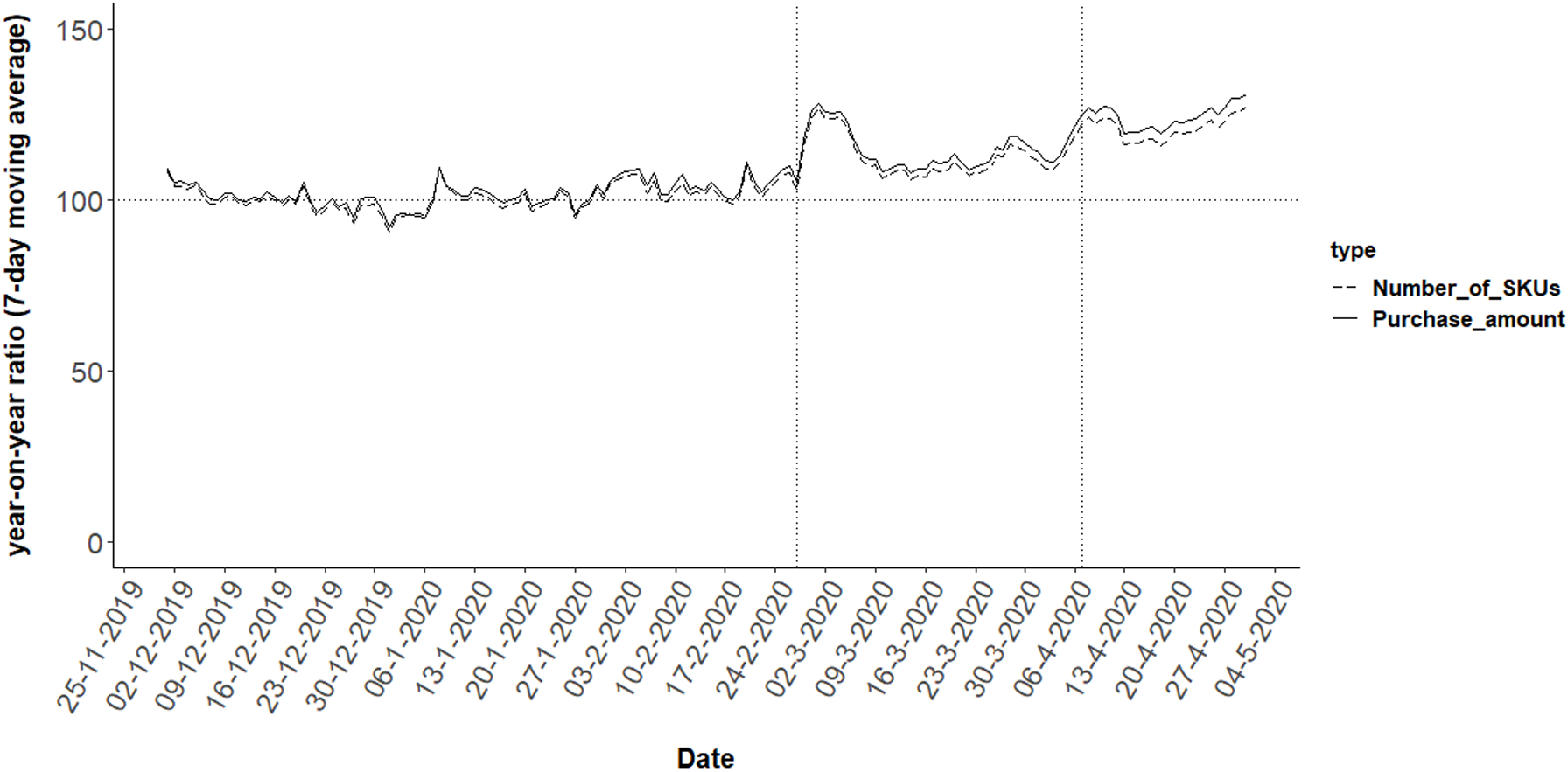
Finally, this study has some limitations that present opportunities for future research. First, our analysis is based on purchase amounts, and we do not refer to the price changes of each product. The reason for this is that precise quantity information is not available for some categories in our data set. For instance, products could be sold individually or in bulk, but the number of units adjusted for size is not documented. For example, with respect to SKUs of toilet paper, we cannot easily distinguish whether it is a pack of 8 or a pack of 12 just from the data we have. Thus, it is difficult to capture SKUs qualitatively and decompose purchase amount into price and quantity in multiple categories. If this problem is solved in future, we would attempt to analyze the relationship of prices and quantities. We do, however, have some support for the fact that the increase in purchase amount is largely the result of an increase in purchase quantity and not due to price increases. Under the assumption that the quality of SKUs is not distinguished, we can show this. Appendix Figure C shows the time series of the year-on-year ratio (7-day moving average) of the number of SKUs purchased, using the same calculation as the purchase amount in Figure 2. From this figure, we can see that the variation in the purchase amount and the number of SKUs purchased are similar.

Second, we did not find a strong relationship between the segment of panic buying and media usage, especially television viewing. A reason may be that we manipulated the media usage variable as consumers’ general habits, rather than media contact related to COVID-19. Although there are limitations to the data used in this study, if we could identify associations between television programs and mobile apps and COVID-19, we could extract more influential data on media usage behavior.

FOOTNOTE

1)  The Syndicated Consumer Index (SCI) is managed by INTAGE Inc. and has been in constant operation since 2012. The sample size used to calculate the indicators in Figure 2 was 38,213. Figure 2 shows the total value of consumer packaged goods, including groceries, beverages, daily necessities, cosmetics, and drugs.

2)  Goldenberg et al. (2002) focused on the following waveform pattern: “an initial peak, then a trough of sufficient depth and duration to exclude random fluctuations, and eventually sales levels that exceeded the initial peak.” They called this a “saddle.”

3)  Strictly speaking, in addition to these, the variable saddle duration was used.

4)  We focus on the total value of consumer packaged goods as the reference value at which at least the temporary purchase increases occurred.

5)  We can see that d condition is valid even with a qualitative check. The categories actually excluded by the d condition, especially in the second wave, are: seasoning (including sauce, sugar, honey, cooking rice wine, spice and condiment), butter, cheese, bacon, roast pork, fresh/boiled noodle, bouillon and consomme. These are categories that are expected to be in constant and ongoing demand due to increased opportunities for eating at home.

ACKNOWLEDGEMENTS

The authors thank the editors and anonymous reviewers for their helpful and constructive suggestions. The authors are also grateful to INTAGE Inc. for providing the data. This research was supported by Japan Society for the Promotion of Science, KAKENHI (19K01947; 19K13835; 21H00759; 22K20145).

Appendix

 

Table A.1 Temporarily hoarded product categories during the first wave

First Wave
No	Product Category	h	d		No	Product Category	h	d
1	household gloves	199.5	107.2		31	insecticide	42.8	44.1
2	sanitary napkins	157.8	118.6		32	wrapping film	42.6	22.8
3	paper towels	157.7	103.2		33	barley tea	41.9	30.3
4	wet tissues	153.0	116.1		34	kitchen drain bags	41.9	22.4
5	facial tissues	111.1	95.5		35	food extracts	40.9	17.4
6	toilet paper	109.8	74.3		36	pet care products	40.7	32.1
7	dried noodles	104.7	58.4		37	stew	40.7	23.8
8	pre-cooked rice	92.9	56.0		38	cooking rice wine	40.1	19.3
9	spaghetti	92.8	51.9		39	canned vegetables	38.3	19.0
10	other household cl.	90.3	58.8		40	salt	37.4	29.2
11	disposable cl. paper	83.5	46.9		41	frozen fruit/veges	33.7	16.3
12	instant noodle packs	81.7	51.7		42	hand and skincare	32.9	16.4
13	pre-mixed flour	79.2	31.5		43	breadcrumbs	31.4	17.6
14	air freshener	76.4	51.8		44	toilet-bowl cleaner	31.2	14.3
15	pasta sauce	75.7	43.6		45	ketchup	31.0	14.8
16	soap	69.0	38.4		46	instant soup	30.7	18.8
17	flour	63.4	27.9		47	mayonnaise	30.5	20.4
18	curry	56.6	36.7		48	tomato juice	30.1	22.6
19	laundry bleach	53.4	29.6		49	health food	29.5	23.9
20	cup instant noodles	52.7	36.0		50	heavy detergent	29.0	20.1
21	ochazuke topping	48.3	34.4		51	frozen prepared food	29.0	16.1
22	aluminum foil	48.0	24.7		52	bath cleaner	27.5	15.2
23	rice	47.6	30.3
24	other sundries	47.6	62.7
25	canned seafood	46.5	19.7
26	canned fruit	45.9	23.6
27	food packages	44.3	17.3
28	dishwashing liquid	44.2	24.8
29	macaroni	43.5	18.8
30	rice seasoning mix	43.4	26.9

Note: This table is sorted in descending order for h-values.

Table A.2 Temporary hoarded product categories during the second wave

Second Wave
No	Product Category	h	d		No	Product Category	h	d
1	household gloves	131.6	30.5		31	rice	42.3	25.0
2	food extracts	121.1	37.4		32	wrapping film	41.9	20.8
3	pre-mixed flour	116.0	24.1		33	whisky	41.4	18.1
4	spaghetti	113.8	41.7		34	hand and skin care	41.1	9.2
5	whipped cream	113.2	20.9		35	beauty and health drinks	40.6	35.3
6	dried noodles	105.3	44.1		36	dishwashing liquid	39.0	5.7
7	flour	96.7	8.3		37	other all-purps seasoning	38.8	12.4
8	air freshener	90.2	36.9		38	toilet paper	38.7	26.4
9	pasta sauce	81.9	30.7		39	bath cleaner	37.2	21.9
10	soap	75.6	10.4		40	soy sauce	37.0	9.4
11	instant noodle packs	72.0	24.8		41	pouch-packed food	36.8	13.4
12	macaroni	68.8	15.9		42	toilet-bowl cleaner	35.9	11.6
13	other household cl.	63.8	25.0		43	seasoning soy sauce	35.8	10.0
14	pre-cooked rice	63.6	28.2		44	kitchen drain bags	34.4	10.8
15	paper towels	61.2	14.4		45	other food products	34.2	7.8
16	sweet rice wine	59.6	22.3		46	cooking/tempura oil	34.1	11.6
17	aluminum foil	58.4	24.5		47	other sundries	33.8	21.3
18	disposable cl. paper	54.2	15.9		48	ponzu sauce	33.4	11.1
19	canned seafood	53.1	13.2		49	instant soup	33.1	10.0
20	food packages	52.7	11.1		50	hair color	32.5	21.7
21	laundry bleach	52.6	24.9		51	kitchen brushes/sponges	32.4	13.5
22	sesame oil	50.9	6.2		52	seaweed	30.9	7.9
23	wet tissues	49.1	14.6		53	dried fish flakes	30.7	6.8
24	starch noodle	48.1	12.4		54	soda	30.4	19.8
25	canned vegetables	47.7	15.1		55	cup instant noodles	30.0	13.6
26	rice seasoning mix	47.0	18.4		56	miso paste	29.9	7.5
27	curry	46.8	20.6		57	frozen seafood	28.5	6.8
28	breadcrumbs	44.3	7.2		58	regular coffee	28.4	13.5
29	powdered stock	43.4	16.2		59	miso/suimono soup	27.8	16.2
30	ochazuke topping	43.1	19.1		60	food seasoning mix	26.9	6.2
					61	hair rinse	26.5	19.6
					62	cat food	26.4	16.5
					63	wine	26.0	8.1

Note: This table is sorted in descending order for h-values.

Table B.1 Increase in purchase amounts by segment (Seg. 1−3)

	Experienced Shoppers		Inactive shoppers		Weak panic buyers
No	First Wave
1	wet tissues	241%	canned fruit	120%	pre-cooked rice	259%
2	flour	224%	paper towel	114%	cooking rice wine	253%
3	hand and skin care	216%	wet tissues	109%	household glove	250%
4	rice seasoning mix	191%	pasta sauce	96%	spaghetti	247%
5	pet care product	177%	rice seasoning mix	95%	facial tissue	244%
6	sanitary napkin	172%	ketchup	94%	kitchen drain bag	220%
7	paper towel	171%	pack instant noodle	91%	laundry bleach	219%
8	pack instant noodle	165%	toilet-bowl cleaner	82%	pet care product	214%
9	food extracts	165%	pre-mixed flour	82%	paper towel	211%
10	facial tissue	165%	macaroni	81%	pre-mixed flour	194%
11	pre-mixed flour	160%	mayonnaise	80%	dish wash	193%
12	other sundries	157%	flour	77%	soap	190%
13	instant soup	155%	frozen fruit/vege	75%	pack instant noodle	188%
14	food package	153%	pre-cooked rice	74%	curry	183%
15	aluminum foil	144%	bath cleaner	70%	other sundries	182%
16	curry	142%	salt	61%	instant soup	182%
17	spaghetti	142%	facial tissue	61%	canned seafood	181%
18	cooking rice wine	141%	stew	57%	bath cleaner	175%
19	wrapping film	140%	instant soup	56%	toilet paper	174%
20	soap	138%	frozen prepared food	54%	frozen fruit/vege	171%
No	Second Wave
1	flour	227%	pouch-packed food	290%	other food products	113%
2	wet tissues	193%	other sundries	226%	sesame oil	97%
3	hand and skin care	192%	pre-mixed flour	215%	starch noodle	97%
4	spaghetti	181%	flour	188%	macaroni	95%
5	powdered stock	174%	sweet rice wine	186%	seaweed	90%
6	pouch-packed food	170%	food package	182%	paper towel	87%
7	paper towel	166%	cooking/tempura oil	176%	miso paste	84%
8	pre-mixed flour	156%	disposable cl. paper	161%	food seasoning mix	82%
9	pack instant noodle	154%	spaghetti	159%	food extracts	78%
10	macaroni	147%	wet tissues	158%	curry	77%
11	aluminum foil	143%	cat food	158%	pre-mixed flour	75%
12	ochazuke topping	140%	bath cleaner	157%	bread crumb	74%
13	other all-purps seasoning	138%	laundry bleach	155%	canned seafood	69%
14	household glove	138%	sesame oil	155%	soda	68%
15	curry	138%	other all-purps seasoning	153%	dried fish flakes	68%
16	pasta sauce	138%	pasta sauce	149%	toilet-bowl cleaner	68%
17	canned vegetable	137%	regular coffee	147%	rice seasoning mix	67%
18	dish wash	137%	soap	144%	miso/suimono soup	67%
19	soy sauce	133%	rice seasoning mix	142%	pack instant noodle	66%
20	Soda	132%	ponzu sauce	138%	household glove	65%

Note: As an additional analysis, in this Table, we calculated the means of q_i1, q_i2, $\stackrel{-}{q_{i1}}$, $\stackrel{-}{q_{i2}}$ by segment and category. The above % values are the mean of q_i1 ÷ the mean of $\stackrel{-}{q_{i1}}\times 100$ at the first wave, the mean of q_i2 ÷ the mean of $\stackrel{-}{q_{i2}}\times 100$ at the second wave.

Table B.2 Increase in purchase amounts by segment (Seg. 4−5)

	Rational shoppers		Strong panic buyers
No
1	household glove	364%	wet tissues	2218%
2	pre-mixed flour	333%	household glove	1801%
3	paper towel	288%	health food	1510%
4	pasta sauce	284%	pet care product	1248%
5	facial tissue	276%	hand and skin care	915%
6	sanitary napkin	265%	rice seasoning mix	745%
7	pack instant noodle	249%	facial tissue	734%
8	spaghetti	245%	toilet paper	720%
9	disposable cl. paper	225%	canned fruit	706%
10	rice seasoning mix	224%	rice	677%
11	other house hold cl.	219%	pre-cooked rice	671%
12	mayonnaise	218%	toilet-bowl cleaner	667%
13	rice	216%	air freshener	593%
14	curry	212%	barley tea	546%
15	other sundries	210%	spaghetti	540%
16	food package	207%	sanitary napkin	529%
17	frozen fruit/vege	207%	heavy detergent	470%
18	ketchup	200%	pack instant noodle	440%
19	heavy detergent	193%	canned seafood	429%
20	canned seafood	191%	macaroni	417%
No
1	beauty healthy drink	372%	household glove	3310%
2	paper towel	371%	wet tissues	1053%
3	dried noodle	368%	food extracts	756%
4	soap	358%	other house hold cl.	629%
5	food extracts	356%	food package	523%
6	rice	347%	soap	522%
7	spaghetti	345%	aluminum foil	442%
8	hand and skin care	342%	spaghetti	394%
9	other all-purps seasoning	340%	pre-mixed flour	354%
10	whisky	338%	other sundries	349%
11	other house hold cl.	332%	sweet rice wine	346%
12	cat food	332%	regular coffee	341%
13	pre-mixed flour	320%	seaweed	339%
14	ochazuke topping	307%	pack instant noodle	318%
15	air freshener	305%	toilet paper	317%
16	food package	304%	canned seafood	295%
17	powdered stock	302%	hair rinse	290%
18	canned vegetable	300%	hand and skin care	287%
19	toilet-bowl cleaner	298%	flour	283%
20	dish wash	283%	frozen seafood	275%

Note: As an additional analysis, in this Table, we calculated the means of q_i1, q_i2, $\stackrel{-}{q_{i1}}$, $\stackrel{-}{q_{i2}}$ by segment and category. The above % values are the mean of q_i1 ÷ the mean of $\stackrel{-}{q_{i1}}\times 100$ at the first wave, the mean of q_i2 ÷ the mean of $\stackrel{-}{q_{i2}}\times 100$ at the second wave.

Figure C

Time series of the year-on-year ratio comparing number of SKUs and purchase amount.

REFERENCES

•  Ailawadi,  K. L.,  Neslin,  S. A., &  Gedenk,  K. (2001). Pursuing the value-conscious consumer: Store brands versus national brand promotions. Journal of Marketing, 65(1), 71–89.
•  Bagozzi,  R. P., &  Yi,  Y. (1988). On the evaluation of structural equation models. Journal of the Academy of Marketing Science, 16(1), 74–94.
•  Bentall,  R. P.,  Lloyd,  A.,  Bennett,  K.,  McKay,  R.,  Mason,  L.,  Murphy,  J., ... &  Shevlin,  M. (2021). Pandemic buying: Testing a psychological model of over-purchasing and panic buying using data from the United Kingdom and the Republic of Ireland during the early phase of the COVID-19 pandemic. PloS ONE, 16(1), e0246339.
•  Bozdogan,  H. (1987). Model selection and Akaike’s Information Criterion (AIC): The general theory and its analytical extensions. Psychometrika, 52, 345–370.
• Cameron, A. C., & Trivedi, P. K. (2005). Microeconometrics: Methods and applications. New York, NY: Cambridge University Press.
•  Cheng,  C. (2004). To be paranoid is the standard? Panic responses to SARS outbreak in the Hong Kong Special Administrative Region. Asian Perspective, 28(1), 67–98.
•  Chua,  G.,  Yuen,  K. F.,  Wang,  X., &  Wong,  Y. D. (2021). The determinants of panic buying during COVID-19. International Journal of Environmental Research and Public Health, 18(6), 3247.
• Collins, L. M., & Lanza, T. S. (2009). Latent class and latent transition analysis: With applications in the social, behavioral, and health sciences. Hoboken, NJ: John Wiley & Sons, Inc.
• Dholakia, U. (2020a). How panic buying affects our personal finances. Psychology Today. https://www.psychologytoday. com/us/blog/the-science-behind-behavior/202003/how-panic-buying-affects-our-personal-finances (Accessed 12/18/2020).
• Dholakia, U. (2020b). Why are we panic buying during the coronavirus pandemic? Psychology Today. https://www. psychologytoday.com/us/blog/the-science-behind-behavior/202003/why-are-we-panic-buying-during-the-coronavirus-pandemic (Accessed 12/18/2020).
•  Forbes,  S. L. (2017). Post-disaster consumption: Analysis from the 2011 Christchurch earthquake. The International Review of Retail, Distribution and Consumer Research, 27(1), 28–42.
•  Fornell,  C., &  Larcker,  D. F. (1981). Evaluating structural equation models with unobservable variables and measurement error. Journal of Marketing Research, 18(1), 39–50.
•  Fraley,  C., &  Raftery,  A. E. (1998). How many clusters? Which clustering method? Answers via model-based cluster analysis. The Computer Journal, 41(8), 578–588.
•  Fritz,  C. E., &  Marks,  E. S. (1954). The NORC studies of human behavior in disaster. Journal of Social Issues, 10(3), 26–41.
•  Frost,  R. O., &  Gross,  R. C. (1993). The hoarding of possessions. Behaviour Research and Therapy, 31(4), 367–381.
•  Gasink,  L. B.,  Linkin,  D. R.,  Fishman,  N. O.,  Bilker,  W. B.,  Weiner,  M. G., &  Lautenbach,  E. (2009). Stockpiling drugs for an avian influenza outbreak: Examining the surge in oseltamivir prescriptions during heightened media coverage of the potential for a worldwide pandemic. Infection Control & Hospital Epidemiology, 30(4), 370–376.
•  Goldenberg,  J.,  Libai,  B., &  Muller,  E. (2002). Riding the saddle: How cross-market communications can create a major slump in sales. Journal of Marketing, 66(2), 1–16.
• Hair, J. F., Black, W. C., Babin, B. J., & Anderson, R. E. (2010). Multivariate data analysis (seventh ed.). Upper Saddle River NJ: Prentice Hall.
•  Hall,  C. M.,  Fieger,  P.,  Prayag,  G., &  Dyason,  D. (2021). Panic buying and consumption displacement during COVID-19: Evidence from New Zealand. Economies, 9(2), 46.
•  Hori,  M., &  Iwamoto,  K. (2014). The run on daily foods and goods after the 2011 Tohoku earthquake: A fact finding analysis based on homescan data. The Japanese Political Economy, 40(1), 69–113.
•  Islam,  T.,  Pitafi,  A. H.,  Arya,  V.,  Wang,  Y.,  Akhtar,  N.,  Mubarik,  S., &  Xiaobei,  L. (2021). Panic buying in the COVID-19 pandemic: A multi-country examination. Journal of Retailing and Consumer Services, 59, 102357.
•  Kemp,  E.,  Kennett‐Hensel,  P. A., &  Williams,  K. H. (2014). The calm before the storm: Examining emotion regulation consumption in the face of an impending disaster. Psychology and Marketing, 31(11), 933–945.
•  Khare,  A.,  He,  Q., &  Batta,  R. (2020). Predicting gasoline shortage during disasters using social media. OR Spectrum, 42(3), 693–726.
•  Kirk,  C. P., &  Rifkin,  L. S. (2020). I’ll trade you diamonds for toilet paper: Consumer reacting, coping and adapting behaviors in the COVID-19 pandemic. Journal of Business Research, 117, 124–131.
•  Lee,  Y. C.,  Wu,  W. L., &  Lee,  C. K. (2021). How COVID-19 triggers our herding behavior? Risk perception, state anxiety and trust. Frontiers in Public Health, 9, 46.
•  Loxton,  M.,  Truskett,  R.,  Scarf,  B.,  Sindone,  L.,  Baldry,  G., &  Zhao,  Y. (2020). Consumer behaviour during crises: Preliminary research on how coronavirus has manifested consumer panic buying, herd mentality, changing discretionary spending and the role of the media in influencing behaviour. Journal of Risk and Financial Management, 13(8), 166.
•  Maheswaran,  D., &  Meyers-Levy,  J. (1990). The influence of message framing and issue involvement. Journal of Marketing Research, 27(3), 361–367.
• Masyn, K. E. (2013). Latent class analysis and finite mixture modeling. In T. D. Little (Ed.), The Oxford handbook of quantitative methods in psychology (pp. 551–611). New York, NY: Oxford University Press.
•  Mawson,  A. R. (2005). Understanding mass panic and other collective responses to threat and disaster. Psychiatry: Interpersonal and Biological Processes, 68(2), 95–113.
• McLachlan, G. J., & Peel, D. (2000). Finite mixture models. New York, NY: John Wiley & Sons.
•  Mehrabian,  A., &  Stefl,  C. A. (1995). Basic temperament components of loneliness, shyness, and conformity. Social Behavior and Personality, 23(3), 253–264.
•  Meyer,  R. J., &  Assunção,  J. (1990). The optimality of consumer stockpiling strategies. Marketing Science, 9(1), 18–41.
• Ministry of Health, Labor & Welfare. (2020). The number of COVID-19 infections in Japan. https://www.mhlw.go.jp/stf/covid-19/kokunainohasseijoukyou.html (Accessed 12/18/2020).
•  Mishra,  A., &  Mishra,  H. (2011). The influence of price discount versus bonus pack on the preference for virtue and vice foods. Journal of Marketing Research, 48(1), 196–206.
•  Naeem,  M. (2020). Do social media platforms develop consumer panic buying during the fear of COVID-19 pandemic. Journal of Retailing and Consumer Services, 58, 102226.
• Notebaert, L. (2020). COVID-19: The psychology of panic buying. University of Western Australia news. http://www.news.uwa.edu.au/2020042812028/uwa-public-policy-institute/covid-19-psychology-panic-buying (Accessed 12/18/2020).
• Novemsky, N. (2020). Why a Pandemic leads to panic buying. Yale Insight. https://insights.som.yale.edu/insights/why-pandemic-leads-to-panic-buying (Accessed 12/18/2020).
•  Prentice,  C.,  Chen,  J., &  Stantic,  B. (2020). Timed intervention in COVID-19 and panic buying. Journal of Retailing and Consumer Services, 57, 102203.
•  Rajkumar,  R. P., &  Arafat,  S. M. (2021). Model driven causal factors of panic buying and their implications for prevention: A systematic review. Psychiatry International, 2(3), 325–343.
•  Rook,  D. W. (1987). The buying impulse. Journal of Consumer Research, 14(2), 189–199.
•  Schwarz,  G. (1978). Estimating the dimension of a model. Annals of Statistics, 6(2), 461–464.
•  Steketee,  G., &  Frost,  R. (2003). Compulsive hoarding: Current status of the research. Clinical Psychology Review, 23(7), 905–927.
• Sterman, J. D., & Dogan, G. (2015). “I’m not hoarding, I’m just stocking up before the hoarders get here.”: Behavioral causes of phantom ordering in supply chains. Journal of Operations Management, 39–40(1), 6–22.
•  Sun,  B. (2005). Promotion effect on endogenous consumption. Marketing Science, 24(3), 430–443.
•  Sun,  B.,  Neslin,  S. A., &  Srinivasan,  K. (2003). Measuring the impact of promotions on brand switching when consumers are forward looking. Journal of Marketing Research, 40(4), 389–405.
•  Winterich,  K. P., &  Haws,  K. L. (2011). Helpful hopefulness: The effect of future positive emotions on consumption. Journal of Consumer Research, 38(3), 505–524.
•  Yoon,  J.,  Narasimhan,  R., &  Kim,  M. K. (2018). Retailer’s sourcing strategy under consumer stockpiling in anticipation of supply disruptions. International Journal of Production Research, 56(10), 3615–3635.
•  Yuen,  K. F.,  Wang,  X.,  Ma,  F., &  Li,  K. X. (2020). The psychological causes of panic buying following a health crisis. International Journal of Environmental Research and Public Health, 17(10), 3513.