Optimizing Spatial Weight Matrices in Spatial Econometrics: A Graph-Theoretic Approach Based on Shortest Path Algorithms

A New York City Application of Crime and Economic Indicators

Abstract

In spatial econometrics, traditional spatial weight matrix (SWM) methods often fail to capture the complex spatial dynamics of large cities. This study optimizes SWM calculations within spatial econometric models, constructing Graph- Based Spatial Weight Matrices (GBSWM) through the Simple Shortest Path Algorithm by analyzing urban road networks, thereby capturing the intricate spatial relationships within the city. The methodology compares the performance of GBSWM with traditional Simple Distanced Spatial Weight Matrices (SDSWM) using Geographically Weighted Regression (GWR) models. The results show that GBSWM significantly outperforms SDSWM in predicting minor crime events (e.g., 'summonses') in New York City. Improved p-values, Pseudo R-squared values, and model accuracy matrices attest to the improved predictive accuracy of GBSWM. These findings demonstrate the superior capability of GBSWM in capturing complex spatial relationships and interactions within urban settings. The integration of graph theory into spatial econometrics represents a theoretical and methodological advancement. The findings of this study are essential for improving the calculation of spatial weigh matrices, providing a more accurate tool for prediction and analysis in spatial econometric models. This result emphasizes the potential of applying graph methods in spatial econometrics, paving the way for implementing more detailed and practical urban spatial analysis.

Introduction

In spatial econometrics, the analysis of complex urban dynamics is crucial, especially in policy decision-making and economic evaluation (Anselin, 2010). Traditional methods for constructing spatial weight matrices (SWMs) are usually based on simple distances, which often do not adequately reflect the complexity of urban spatial structure (ESRI, n.d.-b; Piquero and Weisburd, 2010). This study addresses this limitation by proposing a finer-grained approach that considers the contribution of the urban road network to the connectivity between regions, thus filling in the details of the road network that tend to be neglected in traditional SWM calculations. By embedding intricate road networks into SWM calculations, this study is expected to improve the model's predictive power significantly.

This study aims to optimize the computation of the SWM through a graph theoretic perspective, replacing the traditional simple distance spatial weight matrix (SDSWM) by integrating urban road networks and shortest path algorithms. The differences between the graph-based spatial weight matrix (GBSWM) and SDSWM are compared in a combination of Global Moran's $I$ of spatial autocorrelation analysis (SAA) and geographically weighted regression (GWR) to improve the accuracy of the spatial econometric model in an urban context.

The research methodology includes a comparative analysis between a conventional SWM and a SWM optimized using a graph theory algorithm under the same spatial econometric model. This comparison is essential to validate the effectiveness of graph theory-based approaches in improving the accuracy and robustness of spatial econometric models. This study tests the hypothesis that graph theory can enhance the accuracy and efficacy of spatial econometric models in complex urban environments by considering the crime phenomenon in the New York City study area. Through this methodological framework, this study aims to contribute to spatial econometrics, especially in understanding and modeling urban dynamic spaces, to improve the stability and accuracy of spatial econometric models. The significance of these objectives is that such methodological improvements have the potential to influence urban planning and policy-making and contribute to theoretical advances in spatial econometrics.

Review of Fundamental Concepts

Spatial econometric models

Spatial econometric models are specialized econometric models that incorporate spatial relationships and dependencies within their analytical framework (Anselin, 1988; Mitchell, 2013). These models are essential in addressing many economic phenomena' spatial dependence and heterogeneity. Spatial dependence implies that values influence values observed in one location in neighboring locations, while spatial heterogeneity recognizes the variation in relationships between variables across different areas (Anselin, 2010; LeSage and Pace, 2009). This study includes spatial autocorrelation analysis and geographically weighted regression among many spatial econometric models. These two models allow the exploration of spatial dynamics in economic data and improve the robustness and depth of spatial econometric analysis.

Spatial autocorrelation analysis

Spatial autocorrelation analysis refers to the correlation observed in a measured variable with its own values, and this correlation is a result of the spatial arrangement of neighboring elements. Global Moran's $I$ and Local Moran's $I$ are widely used inferential statistic methods in spatial econometrics for identifying clustering patterns and detecting local anomalies in a variable across a study area (Anselin, 1988; Anselin, Florax, et al., 2004).

Global Moran's $I$ provides a singular metric summarizing spatial autocorrelation, indicating the presence of a clustering pattern for a specific variable throughout the study area. Global Moran's $I$ can be represented in Equation (1) as follows:

  

$$\begin{array}{c}\hfill I=\frac{N}{W}\frac{\sum _{i=1}^N\sum _{j=1}^N{w}_{\mathrm{\text{ij}}}(X_i-\overline{X})(X_j-\overline{X})}{\sum _{i=1}^N{(X_i-\overline{X})}^2}\left(1\right)\hfill \end{array}$$

Here, $N$ is the number of spatial units, $w_{\mathrm{\text{ij}}}$ represents the spatial weight between observations $i$ and $j$ , $X_i$ and $X_j$ are the variable values for observations $i$ and $j$ , and $\overline{X}$ is the mean of the variable (ESRI, n.d.-a).

Local Moran's $I$ identifies specific areas of intense high or low values (hotspots or cold spots), facilitating targeted interventions. It evaluates spatial autocorrelation at the individual unit level. Local Moran's $I$ can be represented in Equation (2) as follows:

  

$$\begin{array}{c}\hfill I_i=\frac{(X_i-\bar{X})\sum _{j=1}^N{w}_{\mathrm{\text{ij}}}(X_j-\bar{X})}{\mathrm{\text{Var}}\left(X\right)}\left(2\right)\hfill \end{array}$$

Both global and local Moran’s $I$ come with statistical tests to assess the significance of the autocorrelation, providing a robust mechanism to validate observations. These statistics describe the tendency for similar values to be clustered across the entire spatial domain or at individual units within the dataset. A value close to $+1$ indicates strong positive spatial autocorrelation, a value close to $-1$ indicates strong negative spatial autocorrelation and a value around zero suggests a random spatial pattern. Ignoring such spatial effects could lead to model misspecification, biased parameter estimates, and incorrect inferences (Anselin, 1988; Anselin, Florax, et al., 2004).

Geographically weighted regression

Geographically Weighted Regression (GWR) is a statistical technique that allows for local parameter estimation rather than global, making it more sensitive to spatial variations in the data. The GWR's location-specific coefficients enable detailed analysis of variable relationships across different areas, proving invaluable in urban planning, environmental science, and epidemiology, where spatial context is vital (Anselin, 1988; Anselin, Florax, et al., 2004; Gollini, Lu, et al., 2015).

By considering the spatial context, GWR often provides better predictive accuracy than traditional regression models that assume stationary relationships. The general form of the GWR model for an observation at location $i$ can be represented in Equation (3) as follows:

  

$$\begin{array}{c}\hfill Y_i={\beta }_{0i}+{\beta }_{1i}{X}_{1i}+{\beta }_{2i}{X}_{2i}+\dots +{\beta }_{\mathrm{\text{ki}}}{X}_{\mathrm{\text{ki}}}+{ϵ}_i\left(3\right)\hfill \end{array}$$

In this model, \text{Y\!}_{i} represents the dependent variable, $X_{1i}$ , $X_{2i}$ …, $X_{\mathrm{\text{ki}}}$ are the independent variables, and ${\beta }_{0i}$ , ${\beta }_{1i}$ …, ${\beta }_{\mathrm{\text{ki}}}$ are the local regression coefficients at location $i$ . The estimation of local regression coefficients is described in Equation (4):

  

$$\begin{array}{c}\hfill {\beta }_i={\left(X_i^T{W}_i{X}_i\right)}^{-1}{X}_i^T{W}_i{Y}_i\left(4\right)\hfill \end{array}$$

Where $W_i$ is the spatial weighting matrix (SWM) centered at location $i$ . The choice of kernel function and bandwidth in GWR affects how the weights decay with distance, influencing the local nature of the model. A small bandwidth will make a model susceptible to local variations but also more susceptible to overfitting. The bandwidth parameter needs careful selection as too large a bandwidth will make the model essentially global, while too small a bandwidth will make it overly sensitive to local noise.

Spatial weights matrices

A spatial weight matrix (SWM), symbolized as $W$ , is a structured representation in spatial econometrics and geography used to quantify the spatial relationships among a set of geographic entities (Anselin, 1988). This matrix is constructed by assigning weights to each pair of entities based on their spatial proximity, contiguity, or other relevant spatial criteria. The calculation of these weights varies: they can be binary (1 for neighboring entities, 0 otherwise), based on inverse distance (where weights decrease with increasing distance, such as Simple Distanced Spatial Weight Matrices (SDSWM)), or other functions capturing specific spatial interactions (ESRI, n.d.-b; Piquero and Weisburd, 2010). The structure of $W$ is typically an $n\times n$ matrix, where $n$ represents the number of spatial units considered. Each element $w_{\mathrm{\text{ij}}}$ in the matrix represents the weight assigned to the spatial relationship between the $i^{\mathrm{\text{th}}}$ and $j^{\mathrm{\text{th}}}$ units. The diagonal elements of this matrix are usually set to zero, indicating that a unit does not have a spatial relationship with itself (Anselin, 1988). The design of $W$ is crucial, as it directly influences the analysis of spatial dependence or autocorrelation.

SWMs play a pivotal role in urban spatial analysis, offering a framework to understand and quantify the relationships and interactions between different areas within a city (LeSage and Pace, 2009; Mitchell, 2013). These matrices are instrumental in evaluating urban areas' prominence and spatial structure, facilitating a more nuanced understanding of urban dynamics. The primary types of SWMs include binary, distance decay, generalized, and k-order neighbors. Each type offers unique advantages and disadvantages. Binary matrices are straightforward to interpret but may oversimplify complex spatial relationships. Distance decay matrices, which factor in the diminishing influence of distance on spatial relationships, provide a more realistic representation of spatial interactions, but they require careful calibration of the decay function. Generalized matrices offer flexibility in defining spatial relationships but can be complex to construct and interpret. K-order neighbor matrices extend the analysis to include broader neighborhood effects, yet this approach might incorporate irrelevant spatial units, potentially diluting the analysis (C. Zhang, 2012).

The choice of weights and the matrix structure must be carefully considered to reflect the underlying spatial dynamics of the data accurately (Florax and De Graaff, 2004). The choice can affect the assessment of area prominence and the interpretation of spatial patterns, thus influencing model application and data analysis (Bauman, Drouet, et al., 2018; X. Zhang and Yu, 2018). While these matrices provide valuable insights into urban structures, their effectiveness is often contingent upon the specific urban context and the objectives of the analysis (Anselin, 2002). Therefore, selecting an appropriate SWM requires careful consideration of the urban area's unique characteristics and the specific goals of the study (Ermagun and Levinson, 2018). The automatic selection of SWMs discussed by Seya, Yamagata, et al. (2013), the autoregressive model with an endogenous SWM proposed by Qu and Lee (2015), and the optimization choices in eigenvector-based methods examined by Bauman, Drouet, et al. (2018) illustrate the evolving methods to improve SWM calculations. These approaches often grapple with the complexities of real-world data and the generalizability of their findings, such as the sensitivity of results to the chosen SWM and the difficulty in capturing the complexity of urban spatial structures (Stakhovych and Bijmolt, 2009).

While existing research provides valuable insights into the spatial nature of understanding spatial econometrics, a clear gap exists in optimizing SWM calculations. The limitations of distance-based and shared boundary-based SWM calculations in such areas call for innovative approaches incorporating urban road network systems, as Ermagun and Levinson (2018) suggested. The abovementioned shortcomings in traditional methods hinder a comprehensive understanding of spatial relationships in urban settings. The failure to adequately account for unique geographical features and road networks in SWM calculations potentially leads to suboptimal predictions in spatial econometric models, thereby impacting the efficacy of policy interventions based on these models.

While effective in specific contexts, traditional SWM approaches often fail to capture the nuanced spatial relationships in complex urban environments, leading to suboptimal predictions and inefficient policy interventions. This problem is significant given the increasing complexity of urban transportation systems and the need for more precise policy formulation and urban planning tools. Innovative approaches are required to incorporate urban road network systems, as highlighted by the groundbreaking work of Getis and Aldstadt (2004). They introduced a new method for constructing SWMs using a local statistics model (LSM) based on the $G_i$ * local statistic. This method emphasizes the importance of considering spatial structures in two parts: those influenced by distance effects and those not. The LSM method, conducted by Getis and Aldstadt (2004), based on the $G_i$ * statistic, effectively identifies critical distances for clustering in spatial data and demonstrates superior performance in identifying spatial structures compared to traditional SWM specifications. This method, showcasing flexibility and adaptability, outperformed traditional SWM specifications in simulation experiments, although its performance in real-world settings requires further exploration.

However, the abovementioned approaches often need to be further revised in complex urban environments, particularly in areas with a complex road network and unique island and peninsula geographic features like New York City, where intricate topographies and diverse socioeconomic landscapes challenge the efficacy of standard SWMs. Therefore, the primary objective of this study is to address the critical gap in optimizing SWM calculations in intricate urban road networks by enhancing the prediction accuracy of spatial econometric models in urban crime analysis by applying graph theory to optimize SWM calculations considering the urban road system. The significance of achieving this objective lies in its potential to offer more precise and context-sensitive econometric models, thereby impacting theoretical frameworks and practical policy-making in urban planning and crime prevention.

Graph theory

Graph theory, a pivotal branch of discrete mathematics, concerns the study of graphs, mathematical structures used to model pairwise relations between objects. A graph in this context comprises vertices (or nodes) and edges (or lines) that connect them. This theory finds applications across various fields, from computer science to social sciences, where it aids in modeling and analyzing networks, such as communication networks, social networks, biological networks, and transport networks. Graph theory algorithms, a critical subset of this field, are procedures or formulas for graph problems (Yannakakis, 1990). These algorithms serve a broad range of purposes, from finding the shortest path between two nodes (as in Dijkstra's or Bellman-Ford algorithms) to detecting cycles (like Tarjan's algorithm for strongly connected components) and determining the most efficient way to 'traverse' or 'visit' each vertex in a graph (illustrated by Eulerian and Hamiltonian path algorithms) (Goldberg and Harrelson, 2005; Han, Wang, et al., 2021; Khuller and Raghavachari, 2010). These algorithms are fundamental in solving complex, real-world problems, offering efficient and effective means to manage and analyze the intricate networks that permeate numerous aspects of modern life.

Graph theoretic algorithms are pivotal in optimizing spatial weight matrices, offering several inherent advantages that make them particularly suitable for complex spatial analyses (Khuller and Raghavachari, 2010). These algorithms efficiently handle complex networks encompassing numerous nodes and connections. This efficiency is crucial when dealing with large datasets where understanding spatial relationships is critical. Moreover, their flexibility and adaptability are notable; they can be tailored to various data types and accommodate different spatial interactions, including adjacency, distance, or flow. This adaptability ensures a broad applicability across various spatial analysis scenarios. Graph theoretic algorithms also provide an accurate and nuanced representation of spatial relationships. Unlike simpler models, these algorithms are adept at capturing direct interactions between areas and the more subtle indirect interactions that can be critical in understanding spatial dynamics. This depth of analysis is essential for a comprehensive understanding of spatial patterns and relationships. Lastly, the scalability of graph algorithms is a significant advantage. As data sizes increase, these algorithms maintain their efficiency and accuracy, making them invaluable for large-scale spatial analyses where traditional methods might falter. This scalability ensures that graph theoretic algorithms remain effective even as the complexity and size of spatial data continue to grow (Yannakakis, 1990).

This study situates itself in filling the existing gap, focusing on integrating graph theory into spatial econometric models, through which this new approach incorporates road network systems into spatial econometric considerations. The graph-based spatial weight matrix (GBSWM), denoted as $W_B$ , is structured to reflect the underlying spatial graph, where nodes represent the spatial units (e.g., regions, districts) and edges symbolize the spatial relationships or connections between these units. The matrix is essential for quantifying the intensity and directionality of spatial interactions, which are pivotal in modeling spatial processes. The elements of $W_B$ are standardized to ensure row-sum consistency, facilitating the interpretation and comparability of spatial effects. Incorporating a GBSWM in spatial econometric models allows for the explicit consideration of spatial autocorrelation, enhancing the robustness and accuracy of inferential statistics derived from spatial data (Yannakakis, 1990).

The expectation of this experimental study is predicated on the hypothesis that integrating graph theory into spatial econometric models, specifically through the development and application of a GBSWM, will significantly enhance the accuracy and efficacy of these models in complex urban environments. This enhancement is anticipated to arise from the GBSWM's ability to more precisely capture the intricate spatial relationships and interactions dictated by urban road network systems. While effective in more straightforward contexts, traditional SWMs often fall short of accurately representing the spatial dynamics within urban areas characterized by complex road networks and unique geographical features. The hypothesis underpinning this study asserts that by incorporating a graph-theoretical approach, the GBSWM will offer a more nuanced and context-sensitive representation of spatial relationships, leading to improved predictive accuracy in spatial econometric models.

Integrating graph theory in optimizing SWM calculations is a pivotal theoretical advancement in addressing the gaps in spatial econometrics. The proposed optimization of SWM calculations through graph theory aligns with and expands upon these existing frameworks. By addressing the unique spatial configurations of urban environments like New York City, this research promises a more accurate and context-sensitive analysis of spatial econometrics analysis, thus offering valuable insights for policy-making and urban planning. This approach, aligning with the theoretical underpinnings of spatial econometrics, offers a nuanced understanding of urban spatial dynamics. Integrating graph theory in optimizing SWM calculations complements existing frameworks like the GWR, potentially enhancing the precision and applicability of these models in complex urban contexts (Stakhovych and Bijmolt, 2009; X. Zhang and Yu, 2018). The experimental study, therefore, aims to empirically validate this hypothesis and demonstrate the superiority of the GBSWM over traditional SWMs in complex urban settings, marking an advancement in spatial econometrics and its application to urban studies.

Experimental Design

This study innovatively applies graph theory to enhance the spatial weighting matrix (SWM) calculation by integrating urban road networks. Graph theory's robust framework is particularly suited for modeling these road networks' intricate, interconnected structures. This approach's reliability hinges on its systematic integration of graph-theoretic principles into the construction and optimization of the SWM, ensuring that spatial dependencies within the urban road network are precisely and nuancedly captured, thereby increasing the accuracy and effectiveness of spatial econometric models (Khuller and Raghavachari, 2010). As a result, the optimized SWM becomes an invaluable tool for a more accurate interpretation of spatial patterns and dynamics.

Data collection and study area

This study used data collected from community districts, street centerlines, complaints, citations, shootings, and economic indicators to test the variability of GBSWM and SDSWM performance through GWR. New York City (NYC) street centerlines are critical for incorporating the physical layout of the roadway network into the spatial weighting matrix, a critical factor in the practical application of graph theory algorithms. Additionally, complaints, citations, and shootings between March 1, 2021, and September 30, 2021, were used as dependent variables in the spatial econometrics model for this study. The New York City Department of City Planning's Economic Indicators dataset and its socioeconomic variables provide essential background information and constitute the independent variables in the spatial econometrics model for this study.

The selection of datasets for this research is strategically aligned to optimize the computation of spatial weight matrices through the integration of road systems, employing graph theory algorithms to enhance the predictive robustness of spatial econometric models. The utilization of Community Districts data from NYC Open Data provides a detailed spatial framework essential for defining the study area and ensuring that the spatial relationships are accurately represented. The data collected from community districts, street centerline, complaint, summons, shooting, and economic indicators are presented in Table 1.

Table 1. Data description

Characteristics	Source	Variable code	Variable description
Community Districts	NYC Open Data (NYC Open Data, 2020)	CD	New York City Community Districts boundaries
NYC Street Centerline	NYC Open Data (NYC Open Data, 2015)	SC	New York City Streets Shapefile Data: address ranges and additional details including traffic direction, roadway type, and segment type
Complaint	NYC Open Data (NYC Open Data, 2023a)	Complaint	Complaint Incident Level Data
Summons	NYC Open Data (NYC Open Data, 2023b)	Summons	Summons Incident Level Data
Shooting	NYC Open Data (NYC Open Data, 2023c)	Shooting	Shooting Incident Level Data
Economic Indicators	NYC Department of City Planning (NYC Department of City Planning, 2021)	Economic Indicators	American Community Survey (ACS) Data Tables: Economic indicators such as income levels, employment status, and housing characteristics

These datasets offer diverse and detailed insights into the dynamics of urban life, which are integral to understanding and modeling spatial interactions within the city. The combined use of these datasets ensures a comprehensive and nuanced approach to spatial econometric modeling, enabling a thorough examination of the interactions within urban environments. This careful selection of data sources substantiates the methodological approach and supports the overall research aim, maintaining an objective and balanced perspective on their use.

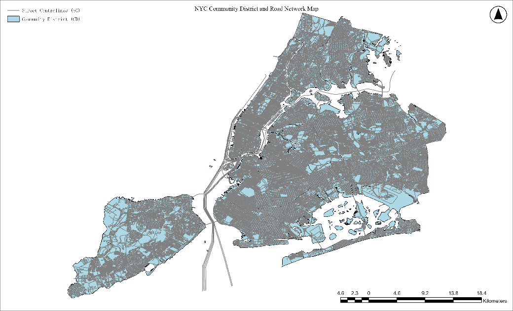
New York City is the selected study area. New York City is in the State of New York, United States, and presents an intricate topography, a complex network of islands and peninsula (Figure 1). Much of New York City is built on three islands: St Staten Island, Manhattan, and Western Long Island. The Hudson River flowing from Hudson Valley into New York Bay becomes an estuary that separates Manhattan and the Bronx from Northern New Jersey. Additionally, the Harlem River separates Manhattan from the Bronx. This metropolis, known for its diverse and densely populated boroughs, offers a multifaceted environment for examining urban phenomena—New York City accounts for five boroughs and is within these 59 community districts. The city's geographical layout poses intriguing challenges for traditional SWM calculations, particularly in understanding and representing the connective dynamics between various urban segments. Additionally, the city's prominent global position and status as a microcosm of urban diversity and complexity make it an ideal subject for spatial studies aiming to generate insights with broader applicability.

Figure 1. NYC Community District and Road Network Map

Experimental steps and explanations

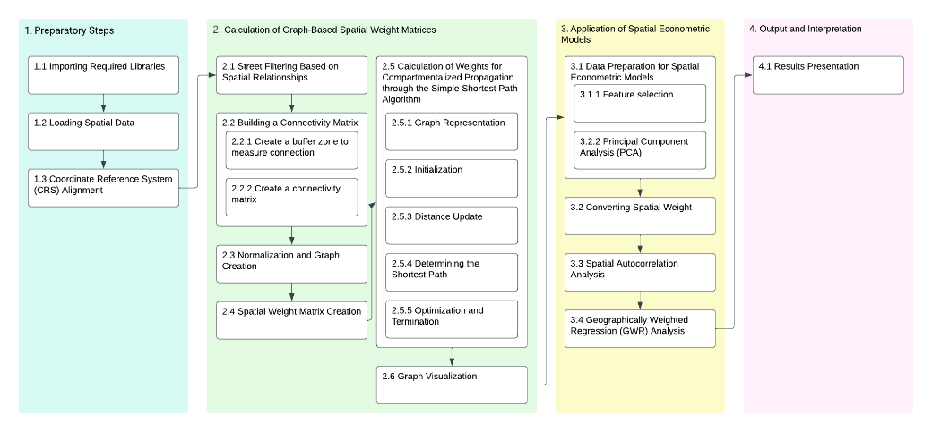
This research is structured around a series of methodologically rigorous steps that collectively form a comprehensive approach to spatial analysis. The experimental study evolved around four phases: 1) the preparatory phase, 2) the calculation of Graph-Based Spatial Weighted Matrices (GBSWM), 3) the application of spatial econometric models, and 4) the interpretations of the results. These phases are presented in Figure 2 and further discussed in the subsections below.

Figure 2. Process Flowchart

Preparatory steps

The experiment involved several libraries, notably Numpy, Pandas, GeoPandas, NetworkX, Seaborn, Matplotlib, PySAL, ESDA, and LibPysal (Anselin, Florax, et al., 2013; Anselin and Hudak, 1992; PySAL Developers, 2018; Rey and Anselin, 2010). Each of these libraries plays a pivotal role in the processing and visualization of spatial data, establishing a robust foundation for subsequent analytical procedures (Bivand, Millo, et al., 2021). The first step shifted to loading spatial data by using GeoPandas. Two primary GeoDataFrames (CD and SC) were loaded in this stage. Subsequently, the coordinate reference system for the community area was confirmed, and the street centerline data were aligned with it. This alignment was imperative to ensure the accuracy and integrity of spatial data and avoid the misalignment of spatial joints caused by the Coordinate Reference System.

Calculation of the Graph-Based Spatial Weight Matrices

The process of calculating graph-based spatial weight matrices commenced with the filtering of streets based on their spatial relationships with community district boundaries. Custom functions were utilized to selectively filter streets that either overlapped or intersected with these boundaries. This filtration was crucial in ensuring the analysis focused solely on spatial interactions relevant to the community districts.

Subsequently, a connectivity matrix ( $M_C$ ) was built. The calculation of the connectivity matrix involved two key steps: Firstly, a buffer zone of 5 meters was created around each street within the selected dataset. The buffer design considers the potential for roads to act as CD boundaries, ensuring that roads that provide connectivity are correctly identified and screened out when connectivity is retrieved. Secondly, using this buffered street data, a connectivity matrix was constructed. This matrix quantified the number of shared buffered streets among community districts, thereby providing a numerical representation of their spatial interconnectivity. The connectivity information gleaned was formatted into an original SWM. The matrix helps to quantitatively represent the direct road connectivity between different community zones and paves the way for the next step of introducing graph theory into SWM calculations.

The third step involved the normalization of the connectivity matrix, followed by the construction of a graph, visually represented to depict the nodes (CD) and their interconnections (edges). This graph was an abstract representation of the community districts and their interconnections, serving as a foundational structure for further spatial analysis. The normalized connectivity matrix is represented in Equation (5):

  

$$\begin{array}{c}\hfill M_C=\left[\begin{array}{cccccc}\hfill 0\hfill & \hfill 0.2558\hfill & \hfill 0.3372\hfill & \hfill 0\hfill & \hfill \cdots \hfill & \hfill 0\hfill \\ \hfill 0.2558\hfill & \hfill 0\hfill & \hfill 0.5348\hfill & \hfill 0.1395\hfill & \hfill \cdots \hfill & \hfill 0\hfill \\ \hfill 0.3372\hfill & \hfill 0.5348\hfill & \hfill 0\hfill & \hfill 0\hfill & \hfill \cdots \hfill & \hfill 0\hfill \\ \hfill 0\hfill & \hfill 0.1395\hfill & \hfill 0\hfill & \hfill 0\hfill & \hfill \cdots \hfill & \hfill 0\hfill \\ \hfill ⋮\hfill & \hfill ⋮\hfill & \hfill ⋮\hfill & \hfill ⋮\hfill & \hfill \ddots \hfill & \hfill ⋮\hfill \\ \hfill 0\hfill & \hfill 0\hfill & \hfill 0\hfill & \hfill 0\hfill & \hfill \cdots \hfill & \hfill 0\hfill \end{array}\right]\#\left(5\right)\hfill \end{array}$$

The research then delved into calculating weights for compartmentalized propagation through the Simple Shortest Path Algorithm, a cornerstone concept in graph theory. In computational graph theory, the Simple Shortest Path Algorithm is a pivotal concept employed to ascertain the most efficient route between two vertices (Khuller and Raghavachari, 2010). The overarching objective is to minimize the path length, typically quantified as the sum of the weights assigned to the edges traversed. The implementation of such algorithms varies, contingent upon the graph's characteristics - whether it is directed or undirected and whether its edges are weighted. Renowned algorithms under this category include Dijkstra's Algorithm, the Bellman-Ford Algorithm, and the Floyd-Warshall Algorithm, each tailored to specific graphs and weight conditions (Khuller and Raghavachari, 2010; Madkour, Aref, et al., 2017).

In the context of this project, the adoption of Dijkstra's Algorithm was driven by the specific attributes of the graph matrix. Dijkstra's Algorithm is renowned for its efficiency in traversing weighted graphs where edge weights are non-negative (Goldberg and Harrelson, 2005). The utilization of this Algorithm was predicated on the fact that the graph matrix is normalized, implying that the weights are standardized and, crucially, non-negative. This normalization eliminates the presence of negative weights, rendering Dijkstra's Algorithm an optimal choice. Its ability to efficiently compute the shortest path from a single source vertex to all other vertices in a weighted graph, coupled with its suitability for graphs with non-negative weights, made it the most viable and effective Algorithm for application (Goldberg and Harrelson, 2005). The process involves graph representation, initialization of nodes with specific distances, iterative updating of shortest distances for neighboring nodes, determining the shortest path by backtracking, and optimization and termination when the shortest paths are identified. The Simple Shortest Path Algorithm confirms the shortest path between each CD and its non-adjacent CDs, which is the unique possibility of the most robust connectivity among the many potential relationships between non-adjacent CDs. Consequently, the most significant correlations between non-neighboring CDs were calculated based on probabilistic reasoning and weighted undirected graphs.

The utilization of multiplicative cumulative weights in spatial analysis, particularly within the context of crime propagation through various geographic compartments, is underpinned by probabilistic reasoning and the nature of spatial relationships as represented in a weighted undirected graph. The foundational premise for this approach lies in the normalization of the original weights as proper fractions, which represent the probabilities associated with the event (such as a crime) transiting from one compartment to another.

In a weighted undirected graph, each edge signifies the likelihood or probability of transition between nodes (or compartments in this context). These probabilities are not arbitrary but are determined by the correlation between two regions in the connectivity matrix. Suppose the likelihood of a crime event traveling from one region to another is directly proportional to the accessibility between the two regions. In that case, the correlation probabilities of our connectivity matrix between the two regions are normalized to reflect the actual likelihood of an event crossing from one node to another. When considering the path that an event, like a criminal activity, takes through a network of compartments, it becomes necessary to compute the probability of traversing through a particular sequence of compartments, making the concept of multiplicative cumulative weights crucial.

The multiplicative nature of these weights is grounded in basic probability theory. When an event moves through multiple independent pathways, the total probability of this sequential occurrence is the product of the probabilities of each pathway. Therefore, in the context of a spatial network, the probability of a crime propagating through a sequence of compartments (or nodes) is determined by multiplying the weights (probabilities) of each edge (pathway) involved in the shortest path through the network. This approach accurately represents the cumulative effect of multiple, interconnected transitions.

Furthermore, this methodology captures spatial interactions and dynamics of a nuanced and compound nature. It considers the direct links between adjacent compartments and the more complex and often less intuitive indirect connections that can significantly influence the spatial behavior of phenomena like crime. By using multiplicative cumulative weights, analysts can more accurately model and understand the probabilistic flow of events through spatial networks, leading to more informed and effective decision-making and planning, especially in fields such as urban development, law enforcement, and public policy.

The GBSWM calculated by the Simple Shortest Path Algorithm is represented in Equation (6):

  

$$\begin{array}{c}\hfill W_G=\left[\begin{array}{cccccc}\hfill 0\hfill & \hfill 0.2558\hfill & \hfill 0.3372\hfill & \hfill 0.0356\hfill & \hfill \cdots \hfill & \hfill 5E-10\hfill \\ \hfill 0.2558\hfill & \hfill 0\hfill & \hfill 0.5348\hfill & \hfill 0.1395\hfill & \hfill \cdots \hfill & \hfill 7E-12\hfill \\ \hfill 0.3372\hfill & \hfill 0.5348\hfill & \hfill 0\hfill & \hfill 0.0002\hfill & \hfill \cdots \hfill & \hfill 2E-10\hfill \\ \hfill 0.0356\hfill & \hfill 0.1395\hfill & \hfill 0.0002\hfill & \hfill 0\hfill & \hfill \cdots \hfill & \hfill 2E-10\hfill \\ \hfill ⋮\hfill & \hfill ⋮\hfill & \hfill ⋮\hfill & \hfill ⋮\hfill & \hfill \ddots \hfill & \hfill ⋮\hfill \\ \hfill 5E-10\hfill & \hfill 7E-12\hfill & \hfill 2E-10\hfill & \hfill 2E-10\hfill & \hfill \cdots \hfill & \hfill 0\hfill \end{array}\right]\left(6\right)\hfill \end{array}$$

Figure 3. Weighted Network Graph through the Simple Shortest Path Algorithm

Lastly, the graph was visualized using NetworkX and Matplotlib as shown in Figure 3. This visualization effectively illustrated the nodes, representing community districts, and the edges, denoting the connections between these districts (Han, Wang, et al., 2021). The employment of such visualization tools was pivotal in providing a graphical representation of the spatial relationships and interactions within the community districts.

Spatial econometric models’ application, output, and interpretation

In the final stage, the results of the spatial econometric model were used to compare the differences between the spatial weight matrices of graph- theoretic optimization and those of traditional methods. The research design advanced by applying spatial weight matrices, a critical component for spatial econometrics analysis models such as spatial autocorrelation and conducting Geographically Weighted Regression (GWR) analysis (Anselin, 1988).

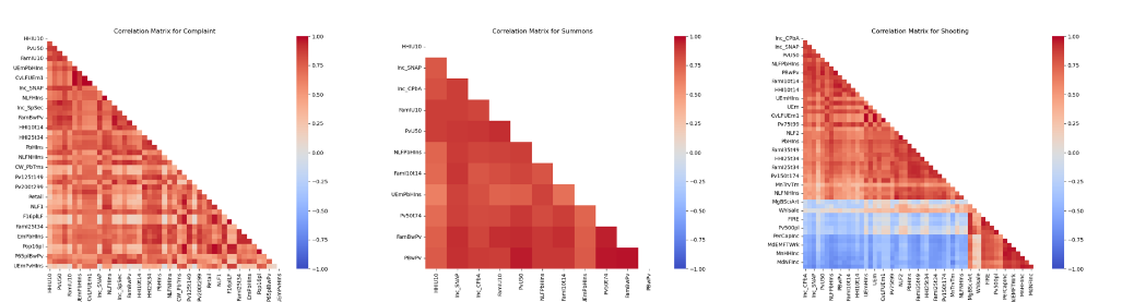
Before these analyses, data preparation encompasses the alignment and normalization of spatial weight matrices and the refinement of economic indicators through feature selection and Principal Component Analysis (PCA) (Hall, 1999). The feature selection process was instrumental in identifying and selecting the most relevant variables for each target variable based on their correlation. The feature selection result is represented in Figure 3. This process simplifies the model and enhances performance by concentrating on the most informative data. PCA, a statistical technique widely used in data analysis and machine learning, was employed for dimensionality reduction while preserving as much of the data's variance as possible. This technique is a powerful feature extraction and reduction tool, facilitating data visualization, model simplification, and performance enhancement.

Figure 4. Dependent Variables Feature Selection Results

The SWMs were then converted into the LibPysal format weight matrix, facilitating their use in spatial econometric analyses (PySAL Developers, 2018; Rey and Anselin, 2010).

Spatial autocorrelation analysis followed, where Moran's $I$ statistic was computed. The computation of Moran's $I$ statistic allows for assessing spatial autocorrelation in various variables (Griffith and Anselin, 1989). This statistic measures spatial autocorrelation, which can be calculated using different spatial weight matrices to gain insight into the spatial relationship between various variables, thus eliminating confounding terms by filtering out variables with significant autocorrelation among several dependent variables.

The final step was implementing GWR analysis. This analytical approach allows for exploring spatial heterogeneity and identifying local variations in the relationships between variables across different geographical areas (Anselin, 1988; Anselin, Florax, et al., 2004). In this experiment, the GWR model was applied for outputting model predictions to compare the performance differences between different SWM approaches.

In the output and interpretation phase, the study analyses the GWR models applied to SWMs before and after optimization. This part of the study involves presenting a concise comparison of the GWR results, highlighting the effects of optimization. It also includes identifying and listing significant variables revealed in the models. The aim is to understand how optimization influences spatial dynamics and interactions within the urban framework, offering insights into the effectiveness of spatial weight matrix optimization in urban spatial analysis.

Experimental Simulation Results

The comparative analysis of Graph-Based Spatial Weight Matrices (GBSWM) and Simple Distanced Spatial Weight Matrices (SDSWM) within Geographically Weighted Regression (GWR) models yields insights into the dynamics of urban spatial interactions. This experiment evaluates the efficacy of GBSWM optimization against the conventional SDSWM in analyzing urban road networks.

The selection of "Shooting" and "Summons" as the primary dependent variables for subsequent analysis in this study is grounded in preliminary findings derived from Spatial Autocorrelation: Moran's $I$ analysis. This initial analysis, focusing on various potential dependent variables, aims to determine the extent of spatial autocorrelation about highly correlated independent variables. The results from this analysis were pivotal in guiding the choice of dependent variables; "Shooting" and "Summons" emerged as the only variables exhibiting statistically significant spatial autocorrelation. This significance underscores their relevance in optimizing spatial weight matrices and validates their selection for detailed examination in the following comparative analysis.

In the comparative analysis of the GBSWMs and SDSWMs for examining "Shooting" and "Summons" incidents, distinct advantages and characteristics emerge. Both models have unique methodological underpinnings: SDSWM calculates weights based on the inverse of distance, whereas GBSWM incorporates the inverse ratio of distance and integrates the road network system, offering a more complex and potentially context-sensitive approach.

Table 2. GWR results for the dependent variable 'Shooting'

	Graph-Based Spatial Weight Matrices	Simple Distanced Spatial Weight Matrices
Dependent Variable p-value	0.003	0.008
Mean dependent var	-0.0053
S.D. dependent var	1.0162
Pseudo R-squared	0.6192	0.6225
Spatial Pseudo R-squared	0.6198	0.6151
Sigma-square ML	0.387	0.383
S.E of regression	0.622	0.619
Log likelihood	-55.683	-55.482
Akaike info criterion	125.366	124.964
Schwarz criterion	139.909	139.506

Table 2 presents the GWR result for the dependent variable 'Shooting', both models demonstrate a commendable ability to explain the variability in the dependent variable, as evidenced by their significant p-values (GBSWM: 0.003 SDSWM: 0.008). This result indicates a robust relationship between the predictors and shooting incidents in both models. The slight edge of SDSWM in terms of Pseudo R-squared (0.6225) over GBSWM (0.6192) is marginal, suggesting that both models are nearly equivalent in their explanatory power. Similarly, while SDSWM exhibits a marginally lower Sigma-square ML and Standard Error (S.E.) of Regression, the differences are minimal, underscoring the comparable precision and error variance in both models.

Table 3. GWR results for the dependent variable ‘Summons’

	Graph-Based Spatial Weight Matrices	Simple Distanced Spatial Weight Matrices
Dependent Variable p-value	0.029	Not Significant
Mean dependent var	0.0133
S.D. dependent var	1.0118
Pseudo R-squared	0.2488	0.2132
Spatial Pseudo R-squared	0.1935	0.1959
Sigma-square ML	0.757	0.792
S.E of regression	0.870	0.890
Log likelihood	-76.148	-77.051
Akaike info criterion	166.297	168.102
Schwarz criterion	180.840	182.645

Table 3 presents the GWR results for the dependent variable ‘Summons’. The GBSWM's superiority becomes pronounced. GBSWM demonstrates statistical significance with a p-value of 0.029, unlike SDSWM, which does not show a significant relationship. This result underscores the enhanced capability of GBSWM in capturing the dynamics related to summons-related incidents. Moreover, GBSWM's performance in terms of lower Sigma-square ML (0.757) and lower S.E. of Regression (0.870) compared to SDSWM (Sigma-square ML: 0.792, S.E.: 0.890) indicates its superior precision in estimation and lower error variance.

Integrating the road network system in GBSWM likely contributes to this enhanced performance of the spatial econometric models, especially in urban studies or geographical analyses where road networks significantly impact spatial relationships. Additionally, GBSWM's better scores in Log Likelihood, Akaike Information Criterion (AIC), and Schwarz Criterion (BIC) for both variables suggest a higher likelihood of the model producing the observed data and a more optimal balance between model complexity and goodness of fit.

While both GBSWM and SDSWM show close performance for the 'Shooting' variable, GBSWM demonstrates a clear advantage in analysing the 'Summons' variable. The marginal differences in performance for 'Shooting' indicate that both models are competent. However, the distinct edge of GBSWM in 'Summons' analysis, particularly in statistical significance and model selection criteria, highlights its suitability for more complex spatial analyses of minor crime events. Including road networks in GBSWM enhances its applicability to diverse urban and geographical contexts and underscores its potential as a more comprehensive tool in spatial modelling.

The comparative analysis between GBSWM and SDSWM reveals intriguing patterns. For instance, GBSWM's integration of road networks suggests a more nuanced understanding of urban spatial dynamics, particularly evident in the 'Summons' data for minor crime events. This result implies that urban planning and policy development should consider spatial interdependencies for more effective outcomes.

The empirical findings delineate differential impacts on the variables 'Shooting' and 'Summons,' with GBSWM demonstrating superior statistical significance and model fit in specific metrics. This outcome of better p-values suggests that the GBSWM approach engenders a model with enhanced statistical robustness. The 'Summons' variable analysis under GBSWM yielded a statistically significant p-value, contrasting with the non-significant result of the SDSWM. Such disparities, particularly in Sigma-square ML and the Standard Error of regression across both models, underscore the distinct methodological impacts attributable to the differing GBSWM constructions.

These empirical outcomes are congruent with the previous theoretical postulates, particularly the premise that graph-theoretical approaches can augment the comprehension of spatial interdependencies within urban matrices. The apparent superiority of GBSWM in certain aspects corroborates the hypothesis that a more intricate portrayal of spatial interactions is beneficial, thus supporting and extending the traditional SWM application paradigms in econometric analyses.

Conclusions, Limitations, and Further Research

Conclusions

This study presents an advancement in spatial econometrics by integrating graph theory with traditional spatial econometric methodologies. The application of Graph-Based Spatial Weight Matrices (GBSWM) has enhanced the prediction accuracy and ubiquity of spatial econometric models in this context. Through comparative analysis with Simple Distanced Spatial Weight Matrices (SDSWM), the superior capability of GBSWM in capturing complex spatial relationships in urban settings has been demonstrated. In doing so, the study utilized crime and spatial phenomena in its to examination. Compared to traditional spatial weighting matrices, the GBSWM improves the interpretability and accuracy of modeling minor crime incidents without significantly negatively affecting the analysis of serious crime incident data guided by traditional methods. This result is particularly evident in the study comparisons.

The significance of this research lies in its theoretical and methodological contributions to spatial econometrics. Blending graph theory into SWM offers novel insights into urban spatial analysis, emphasizing the importance of considering intricate road network interdependencies for effective policymaking. These findings also provide practical implications for urban planning, law enforcement strategies, and policy interventions in densely populated areas.

Based on these findings, applying GBSWM presents a promising avenue for enhancing analytical models, particularly in understanding and managing urban phenomena for scholars and professionals in spatial econometrics. Integrating GBSWM can refine models forecasting urban economic indicators, offering more precise and extensive tools for economic policymakers and urban planners. The GBSWM enables scholars to gain a nuanced understanding of spatial dependencies and interactions under varying environmental conditions, thereby methodologically facilitating and supporting specific case studies. This advancement contributes to addressing complex issues such as urban expansion, land use planning, and environmental sustainability, as well as enhancing existing road network analyses, including assessments of transportation efficiency and modal analysis of travel (Chen, Yuan, et al., 2023; Eom and Suzuki, 2019; Li, Zhao, et al., 2016).

This research underscores the evolving nature of spatial econometrics and highlights the potential of methodologies like graph theory in enriching our understanding of complex urban phenomena. As cities continue to grow and evolve, the importance of sophisticated spatial analysis tools becomes increasingly paramount. This study contributes to spatial econometrics and paves the way for more nuanced and contextually relevant urban policymaking, ultimately enhancing our capacity to create safer and more resilient urban environments.

Limitations and further research

The methodological framework of the study, delineated by the application of GBSWM for analyzing urban road networks, represents a significant progression in spatial analysis. However, this approach encounters several limitations. A primary limitation concerns the generalizability of the findings. The concentration on urban road networks might not seamlessly translate to disparate types of spatial networks or diverse urban environments, particularly in rural locales where the nature of road networks and spatial interplays substantially diverge that the infrastructure of rural roads frequently leads to direct or indirect socio-economic effects on the population (Wagale, Singh, et al., 2021). This specificity engenders queries regarding the applicability of the study's conclusions across varied spatial structures. Additionally, the research confronts constraints linked to the intrinsic assumptions and sensitivities inherent in Geographically Weighted Regression (GWR) models. GWR models, especially those incorporating GBSWM, exhibit sensitivity to data and bandwidth selection, the application context, and the SWM computation. These elements can profoundly affect model outcomes, potentially leading to challenges like overfitting, particularly in models designed to encapsulate intricate spatial relationships. These sensitivities may impinge upon the robustness and veracity of the research's findings. Furthermore, the research's comparative analysis is primarily confined to juxtaposing GBSWM with SDSWM, limiting insights into GBSWM's efficacy relative to a broader spectrum of spatial weight matrix methodologies or econometric models and a thorough appraisal of GBSWM's position within the spatial analysis techniques. Addressing these limitations is imperative for a more holistic and critical evaluation of the research's methodological advancements.

Given the identified limitations, future research should bridge these gaps and further test the potential of GBSWM in more expansive contexts. Firstly, there is a need to expand the scope of GBSWM's application across different spatial networks and in various urban and rural settings. Such exploration would provide valuable insights into the model's adaptability and versatility across diverse geographical landscapes and varying spatial data types. Secondly, enhancing the computational efficiency of GBSWM stands as a critical objective. This improvement could be achieved by developing more streamlined algorithms and creating simplified models that maintain the core aspects of graph-based approaches while reducing computational burdens. Such advancements would render GBSWM more accessible and practical for a broader user base. Thirdly, there is a compelling opportunity to explore the integration of GBSWM with other spatial econometric models or urban planning tools. This integration could lead to the development of hybrid models that amalgamate the strengths of GBSWM with those of other established methodologies, offering a more comprehensive approach to spatial analysis. Fourthly, addressing the sensitivity and robustness of the model is crucial. Refining the GWR methodologies to overcome challenges like bandwidth selection and model overfitting is essential. Establishing guidelines or best practices for model selection and parameterization in GBSWM applications would greatly benefit practitioners. Lastly, conducting comparative studies of GBSWM against various spatial weight matrix methods and other spatial econometric models is necessary. Such comparative analyses would yield more profound insights into the relative strengths and weaknesses of GBSWM, aiding in its accurate positioning within the spectrum of spatial analysis tools.

The abovementioned improvements would broaden the scope of spatial econometric models and contribute to a more comprehensive understanding of urban and environmental issues. Addressing the sensitivity of these models and conducting comparative studies with alternative approaches are also essential steps to contextualize and refine the insights drawn from this research. By tackling these areas, future research can significantly enhance the understanding and efficacy of GBSWM in spatial econometrics, paving the way for more sophisticated and comprehensive urban spatial analysis.

Author Contributions

Conceptualization, Y.S.; methodology, Y.S.; software, Y.S.; resources, Y.S.; data collection, processing, and analysis, Y.S.; writing—original draft preparation, Y.S.; writing—review and editing, A.C. All authors have read and agreed to the published version of the manuscript.

Ethics Declaration

The authors declare that they have no conflicts of interest regarding the publication of the paper.

Acknowledgments

This research did not receive any grant from funding agencies in the public, commercial, or governmental sectors.

I would like to express my great appreciation to International Review for Spatial Planning and Sustainable Development (IRSPSD) for the valuable and constructive comments and suggestions for improving this research paper.

References

•  Anselin,  L. (1988). Spatial econometrics: Methods and models (Vol. 4). Springer Science and Business Media.
•  Anselin,  L. (2002). Under the hood Issues in the specification and interpretation of spatial regression models. Agricultural Economics, 27(3), 247–267. doi: https://doi.org/10.1111/j.1574-0862.2002.tb00120.x
•  Anselin,  L. (2010). Thirty years of spatial econometrics. Papers in Regional Science, 89(1), 3–25.
•  Anselin,  L.,  Florax , R. J. G. M., et al. (2004). Econometrics for Spatial Models: Recent Advances. In: Anselin, Florax, et al. (eds.), Advances in Spatial Econometrics: Methodology, Tools and Applications, Springer, 1–25. doi: https://doi.org/10.1007/978-3-662-05617-2_1.
• Anselin, L., Florax, R., et al. (2013). Advances in spatial econometrics: Methodology, tools and applications. Springer Science and Business Media.
•  Anselin,  L., and  Hudak,  S. (1992). Spatial econometrics in practice: A review of software options. Regional Science and Urban Economics, 22(3), 509–536. doi: https://doi.org/10.1016/0166-0462(92)90042-Y.
•  Bauman,  D.,  Drouet,  T., et al. (2018). Optimizing the choice of a spatial weighting matrix in eigenvector‐based methods. Ecology, 99(10), 2159–2166. doi: https://doi.org/10.1002/ecy.2469.
•  Bivand,  R.,  Millo,  G., et al. (2021). A Review of Software for Spatial Econometrics in R. Mathematics, 9(11), Article 11. doi: https://doi.org/10.3390/math9111276.
•  Chen,  Y.,  Yuan,  R., et al. (2023). Research on the influencing factors of elderly pedestrian traffic accidents considering the built environment. International Review for Spatial Planning and Sustainable Development, 11(1), 44–63. doi: https://doi.org/10.14246/irspsd.11.1_44
•  Eom,  S., and  Suzuki,  T. (2019). Spatial distribution of pedestrian space in central Tokyo. International Review for Spatial Planning and Sustainable Development, 7(2), 108–124. doi: https://doi.org/10.14246/irspsda.7.2_108
•  Ermagun,  A., and  Levinson,  D. (2018). An Introduction to the Network Weight Matrix. Geographical Analysis, 50(1), 76–96. doi: https://doi.org/10.1111/gean.12134
• ESRI. (n.d.-a). How Spatial Autocorrelation (Global Moran’s I) works—ArcGIS Pro | Documentation. Retrieved from https://pro.arcgis.com/en/pro-app/latest/tool-reference/spatial-statistics/h-how-spatial-autocorrelation-moran-s-i-spatial-st.htm on February 1, 2024.
• ESRI. (n.d.-b). Spatial weights—ArcGIS Pro | Documentation. Retrieved from https://pro.arcgis.com/en/pro-app/latest/tool-reference/spatial-statistics/spatial-weights.htm on October 31, 2023.
•  Florax, R. J. G. M., , and  De Graaff, T. (2004). The Performance of Diagnostic Tests for Spatial Dependence in Linear Regression Models: A Meta-Analysis of Simulation Studies. In: Anselin, Florax, et al. (eds.), Advances in Spatial Econometrics, Springer Berlin Heidelberg, 29–65. doi: https://doi.org/10.1007/978-3-662-05617-2_2.
•  Getis,  A., and  Aldstadt, J. (2004). Constructing the Spatial Weights Matrix Using a Local Statistic. Geographical Analysis, 36(2), 90–104. doi: https://doi.org/10.1111/j.1538-4632.2004.tb01127.x.
•  Goldberg , A. V., and  Harrelson,  C. (2005). Computing the shortest path: A search meets graph theory. SODA, 5, 156–165. doi: https://faculty.cc.gatech.edu/~thad/6601-gradAI-fall2012/02-search-Goldberg03tr.pdf.
•  Gollini,  I.,  Lu,  B., et al. (2015). GWmodel: An R Package for Exploring Spatial Heterogeneity Using Geographically Weighted Models. Journal of Statistical Software, 63(17). doi: https://doi.org/10.18637/jss.v063.i17.
•  Griffith, D. A., and  Anselin, L. (1989). Spatial Econometrics: Methods and Models. Economic Geography, 65(2), 160. doi: https://doi.org/10.2307/143780.
•  Hall , M. A. (1999). Correlation-based feature selection for machine learning [Thesis, The University of Waikato]. Retrieved from https://researchcommons.waikato.ac.nz/handle/10289/15043.
•  Han,  P.,  Wang,  J., et al. (2021). A Graph-based Approach for Trajectory Similarity Computation in Spatial Networks. Proceedings of the 27th ACM SIGKDD Conference on Knowledge Discovery and Data Mining, 556–564. doi: https://doi.org/10.1145/3447548.3467337
•  Khuller,  S., and  Raghavachari,  B. (2010). Basic graph algorithms. In: Algorithms and theory of computation handbook: General concepts and techniques, 7–7. Retrieved from https://dl.acm.org/doi/pdf/10.5555/1882757.1882764
• LeSage, J., and Pace, R. K. (2009). Introduction to spatial econometrics. Chapman and Hall/CRC.
•  Li, Z.,  Zhao,  L., et al. (2016). Highway Transportation Efficiency Evaluation for Beijing-Tianjin-Hebei Region Based on Advanced DEA Model. International Review for Spatial Planning and Sustainable Development, 4(3), 36–44. doi: https://doi.org/10.14246/irspsd.4.3_36.
•  Madkour,  A.,  Aref , W. G., et al. (2017). A Survey of Shortest-Path Algorithms (arXiv:1705.02044). arXiv. Retrieved from http://arxiv.org/abs/1705.02044.
• Mitchell, W. F. (2013). Introduction to spatial econometric modelling. Centre of Full Employment and Equity, University of Newcastle.
• NYC Department of City Planning. (2021). Planning-Population-American Community Survey-DCP. Retrieved from https://www.nyc.gov/site/planning/planning-level/nyc-population/american-community-survey.page.page.
• NYC Open Data. (2015). NYC Street Centerline (CSCL). NYC Open Data. https://data.cityofnewyork.us/City-Government/NYC-Street-Centerline-CSCL-/exjm-f27b
• NYC Open Data. (2020). Community Districts. NYC Open Data. https://data.cityofnewyork.us/City-Government/Community-Districts/yfnk-k7r4.
• NYC Open Data. (2023a). NYPD Complaint Data Current (Year To Date) | NYC Open Data. https://data.cityofnewyork.us/Public-Safety/NYPD-Complaint-Data-Current-Year-To-Date-/5uac-w243.
• NYC Open Data. (2023b). NYPD Criminal Court Summons Incident Level Data (Year To Date) | NYC Open Data. https://data.cityofnewyork.us/Public-Safety/NYPD-Criminal-Court-Summons-Incident-Level-Data-Ye/mv4k-y93f.
• NYC Open Data. (2023c). NYPD Shooting Incident Data (Year To Date) | NYC Open Data. https://data.cityofnewyork.us/Public-Safety/NYPD-Shooting-Incident-Data-Year-To-Date-/5ucz-vwe8.
• Piquero, A. R., and Weisburd, D. (eds.). (2010). Handbook of Quantitative Criminology. Springer New York. doi: https://doi.org/10.1007/978-0-387-77650-7.
• PySAL Developers. (2018). Libpysal.weights.W — libpysal v4.9.2 Manual. Retrieved from https://pysal.org/libpysal/generated/libpysal.weights.W.html.
•  Qu, X., and  Lee,  L. (2015). Estimating a spatial autoregressive model with an endogenous spatial weight matrix. Journal of Econometrics, 184(2), 209–232.
•  Rey, S. J., and  Anselin, L. (2010). PySAL: A Python Library of Spatial Analytical Methods. In: Fischer and Getis (eds.), Handbook of Applied Spatial Analysis: Software Tools, Methods and Applications, Springer, 175–193. doi: https://doi.org/10.1007/978-3-642-03647-7_11.
•  Seya,  H.,  Yamagata,  Y., et al. (2013). Automatic selection of a spatial weight matrix in spatial econometrics: Application to a spatial hedonic approach. Regional Science and Urban Economics, 43(3), 429–444.
•  Stakhovych,  S., and  Bijmolt , T. H. A. (2009). Specification of spatial models: A simulation study on weights matrices. Papers in Regional Science, 88(2), 389–408. doi: https://doi.org/10.1111/j.1435-5957.2008.00213.x.
•  Wagale,  M.,  Singh , A. P., et al. (2021). Socio-economic impacts of low-volume roads using a mixed-method approach of PCA and Fuzzy-TOPSIS. International Review for Spatial Planning and Sustainable Development, 9(2), 112–133. doi: https://doi.org/10.14246/irspsda.9.2_112.
•  Yannakakis,  M. (1990). Graph-theoretic methods in database theory. Proceedings of the Ninth ACM SIGACT-SIGMOD-SIGART Symposium on Principles of Database Systems, 230–242. doi: https://doi.org/10.1145/298514.298576.
•  Zhang,  C. (2012). Spatial Weights Matrix and its Application. Journal of Regional Development Studies, 15, 85–97.
•  Zhang,  X., and  Yu, J. (2018). Spatial weights matrix selection and model averaging for spatial autoregressive models. Journal of Econometrics, 203(1), 1–18.