A New Control Volume-based 2D Method for Calculating the Temperature Distribution of Rod during Multi-pass Hot Rolling

Abstract

A simplified numerical model which can evaluate the 2D temperature distribution of a cross-section in multi-pass hot rod rolling process has been established. The grid of cross-section of workpiece under rolling was remeshed based on the energy rate balance of corresponding control volume. This method gives a quick way for the solution of heat-transfer during hot forming process, and can be applied to the on-line calculation. The validity of this method has been examined by FEM simulation and industrial measurement. The cross-sectional areas (elongations) and temperatures of workpiece calculated by the new method were in agreement with those obtained by the comparison methods.

1. Introduction

Hot rolling of rods is one of the most important manufacture methods of steel. Considerable researches have been devoted to improving the quality of hot rolled products by mathematical models as well as by experimental works. However, most of these models were developed based on the finite element method (FEM) for off-line optimization, such as procedure design and practice improvement, because FEM solves the thermo-mechanical process of metal forming with long computational time. Few works were concerned with the real-time process control. Kwon et al.¹⁾ optimized the process design of bar rolling by temperature prediction model based on lumped heat capacity system. Lee et al.²⁾ presented an 1D heat-transfer model for thermo-mechanical controlled process in rod rolling based on equivalent round section at each pass. There is no report about modeling the rolling process with noncircular cross-sectional shape and with different heat flux around the circumference. So it is necessary to develop a model that can describe the thermal process of noncircular rod rolling, and can be solved accurately, rapidly and stably.

This paper presents a new 2D numerical method for calculating the temperature distribution of rod during multi-pass hot rolling based on control volume method (CVM). A special algorithm was employed to remesh the deformed grid of workpiece under rolling to obtain its discretization equations. The solution of this method was compared with FEM simulated results and industrial measured values.

2. Development of the Method

Figure 1 shows the flowchart for calculating heat transfer process of multi-pass hot rolling. Because the workpiece velocity changes during deformation, the displacement step (ΔL) is used instead of the time step (Δt). The geometry of deformed workpiece is determined by empirical equations without using iterative solution like FEM. Then the grid is updated from calculated geometrical parameters. With the corresponding additive time step, a subroutine is called to calculate the temperature distribution for every control volume. In summary, the whole process of the method includes three basic parts, and the details of each part are discussed as follows.

Fig. 1.

Flow chart representing the calculation process of the new numerical method.

2.1. Temperature Model

Under the assumption that there is no longitudinal temperature gradient, the governing heat transfer equation of workpiece in polar coordinates (r-θ ) can be expressed as   

$$\rho C_{\text{p}}\frac{\partial T}{\partial t}=\frac{1}{r}\frac{\partial }{\partial r}\left(rk\frac{\partial T}{\partial r}\right)+\frac{1}{r}\frac{\partial }{\partial \theta }\left(\frac{k}{r}\frac{\partial T}{\partial \theta }\right)+S$$(1)

where, T and t are the temperature and time, respectively; ρ, C_p, k are the density, specific heat capacity and thermal conductivity of steel, respectively; S is the source term (e.g. deformation heat).

The boundary conditions can be described as follows.

At the center,   

$$t\text{>0, }r\text{ = 0: }-k\frac{\partial T}{\partial r}=0$$

At the free surface   

$$t\text{>0, }r=D/2\text{: }-k\frac{\partial T}{\partial r}=h\left(T-T_{\infty }\right)+{\mathit{\epsilon }}_{\text{s}}{\sigma }_0(T^4-T_{\text{sur}}^4)$$

At the contact surface   

$$t\text{>0, }r=D/2\text{: }-k\frac{\partial T}{\partial r}=h_{\mathrm{c}}\left(T-T_{\mathrm{r}}\right)-cQ$$

where, D is the diameter of rod; h is the convection heat-transfer coefficient; h_c is the total contact conductance; ε_s is the total emissivity; σ₀ is Stefan-Boltzman constant; Q is the heat produced through fiction; c is the partition coefficient of workpiece; T_∞ is the fluid temperature; T_sur is the surroundings temperature; T_r is the surface temperature of roller.

The discretization equations can be derived by integrating Eq. (1) over the control volume and over the interval time. With the initial distribution of temperature, the unknown values of each grid-point can be solved step by step with interval time. The solution of discretization equations was detailed by Patankar,³⁾ and will not be dealt with here.

2.2. Grid Remeshing Algorithm

Figure 2 illustrates the schematic description of rod rolling (round-oval pass). H_i and W_i are the maximum height and maximum width of incoming workpiece, respectively. H_o and W_o are the maximum height and maximum width of deformed workpiece, respectively. R_w is the curvature radius of incoming workpiece. R_g is the radius of roll groove. R_f is the radius of free surface of deformed workpiece.

Fig. 2.

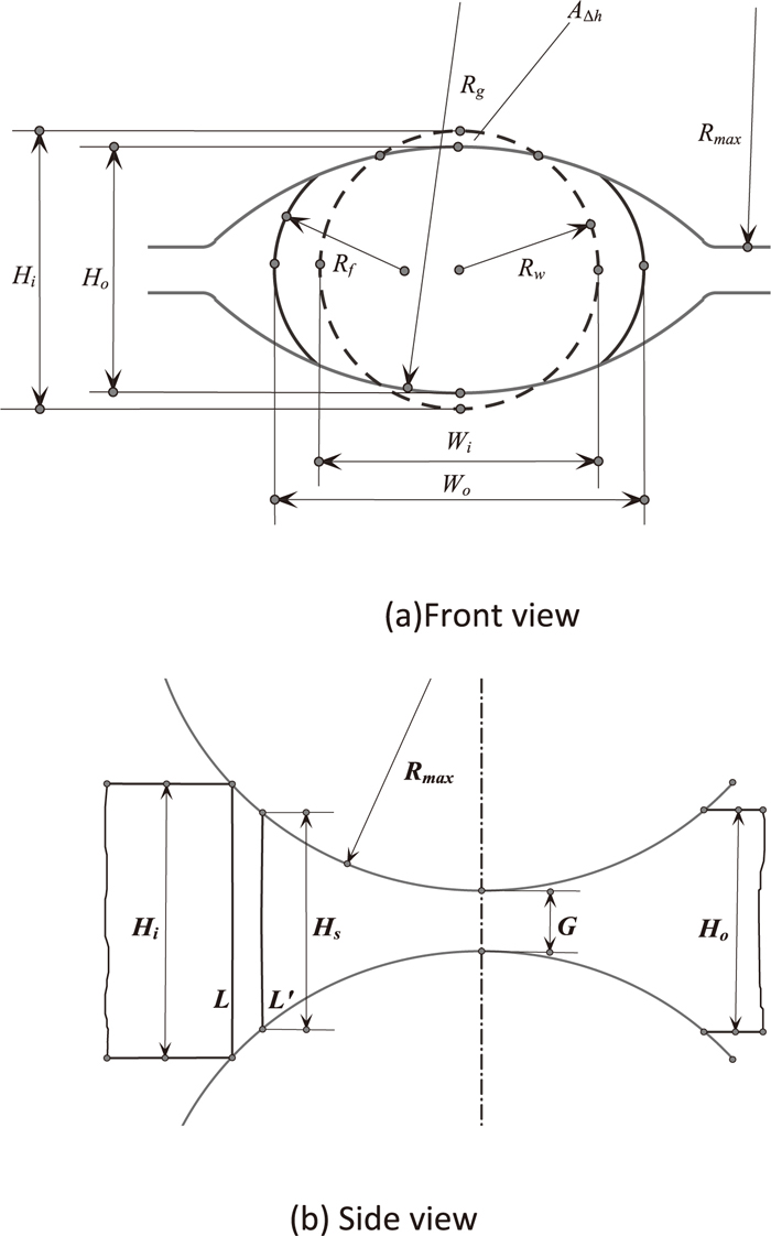
Geometrical designation of a round workpiece incoming into an oval groove.

The grid remeshing algorithm presented in this article includes two steps: adjusting the angular coordinates of boundary points from the control volume of initial grid and calculating the radial coordinates of all points from their constant ratios to boundary points. The following paragraphs give details of this algorithm, along with the proof of keeping control volumes constant.

Take a cross-section of workpiece with unit length as example, when it moves from position L to L′, its shape and size change with deformation process, but its volume remains constant: A_old*1=A_new*e. Where, A_old is the area of initial cross-section, A_new is the area of deformed cross-section, e is the elongation calculated from position L to L′.

Take the symmetry into account, only quarter of the cross-section needs to be calculated. The schematic of initial discrete grid is shown in Fig. 3(a). A typical point P (r_p, θ_p) has the same angular coordinate (θ) with the neighbor points N and S, and has the same radial coordinate ratio to the corresponding boundary point (c_p) with the neighbor points W and E:   

$$r_{\mathrm{P}}/r_{\mathrm{N}}=r_{\mathrm{W}}/r_{\mathrm{Y}}=r_{\mathrm{E}}/r_{\mathrm{B}}=c_{\mathrm{P}}$$

According to the geometric similarity, the area of circle sector A_ONY equals to A_OPW*(c_P)².

Fig. 3.

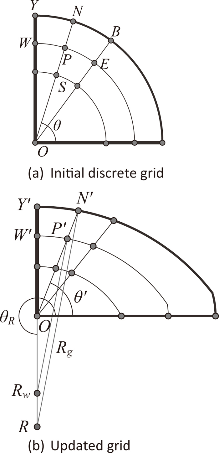
Schematic of the algorithm to remesh the grid after deformation.

To obtain the discretization equation of new cross-section, the angular coordinate of point N is adjusted from θ to θ′, such that the area A_O′N′Y′ equals to A_OYN/e. The new radial coordinates of point Y’ and N’ can be determined from the new cross-sectional profile, which is a circle arc with the center at point R (r_R, θ_R). Then, adjust the radial coordinate of W′ to keep the same ratio to point Y′: r_W′/r_Y′ = r_W/r_Y.

Construct a circle through point W’ with the center at point (c_P*r_R, θ_R), and it intersect the line ON’ at point P’. According to the geometric similarity, we can obtain the relations: r_P′/r_N′ = c_P, and A_O′P′W′ = A_O′N′Y′/(c_P)² = A_OPW/e. It means that the control volume of cell (Y′N′P′W′) equals to that of cell (YNPW).

In similar ways, each cell in initial grid can be modified to the new cell in deformed grid with the same control volume by this method.

2.3. Surface Profile Determination

There is no report about how to calculate the surface profile of workpiece during rolling without using FEM, which will spend at least several hours for a single pass. But a number of studies with empirical formulas have been presented for calculating the exit spread after rolling. So we improved an appropriate one of these formulas to determine the cross-sectional profile of workpiece under rolling.

Shinokura et al.⁴⁾ developed an experimental formula to calculate the maximum spread of workpiece for shape rolling   

$$W_{\mathrm{o}}=b_1\frac{L_{\text{dm}}}{W_{\mathrm{i}}+0.5H_{\mathrm{i}}}\cdot \frac{A_{\mathrm{\Delta }h}}{A_{\mathrm{i}}}$$(2)

where, L_dm is the mean projected arc of contact surface at exit, A_Δh is the cross-sectional area of fractional reduction at exit, A_i is the area of incoming workpiece section, b₁ is a coefficient which is assigned to different pass types. Substituting L_dm and A_Δh at position L′ (see Fig. 2) for the values at exit, the corresponding maximum spread during rolling was solved. Then the analytical models of Lee et al.,⁵⁾ which has improved through substituting the roll gap G by the roll distance H_s at point L′, can be used to obtain the approximate surface profile of deformed workpiece. With the calculated results, the elongation, cross-sectional area and velocity were determined to obtain the new radial coordinate of surface points.

3. Errors and Stability

The temperature model is solved based on the numerical method, CVM. Numerical method can lead to the numerical errors including truncation errors and round-off errors, which have been analyzed extensively, and no further discussed is needed in this paper. The further details can be referenced from Chapra et al.⁶⁾

When the grid is updated, the temperature of each cell is inherited from previous grid, but it may not be a best representative value of the control volume. In order to decrease this inaccuracy, the angular node number and displacement step length were determined by additional sensitivity analysis. The temperature variation along the radial direction is steeper than that along the angular direction, especially near the boundary, so the radial distance of mesh near the surface was reduced accordingly.

The surface profile under rolling, which is calculated from the improved experience formulas, may not be in good agreement with the actual values. To avoid the error propagation within each pass, the substituted variables in each formula were calculated from the mill entrance instead of the previous step. In the mill exit, most of these errors were attenuated because the formulas had been validated at this position.

With workpiece size reduced, the finial rolling velocity increases many times than initial velocity. Unsuitable time step which is calculated from displacement step may cause instability and long-time consumption of calculation. So the appropriate values for each stage were pre-set to acquire a better performance.

There is only one function involving the iteration method, which is used to solve the new angular coordinates in grid remeshing algorithm. But in practice, the approach converged rapidly on the solution within several steps with the Newton-Raphson method, and spent little additional time.

4. Validations

4.1. Compared with FEM Simulation Results

An example of the shape rolling through two mills was performed with the new method and FEM. The workpiece with the initial diameter of 99 mm spends about 11.2 s through two mills, and its diameter is reduced to 72 mm. The code of the new method was implemented in MATLAB, a numerical computing environment from MathWorks. The number of workpiece elements is 100, the displacement step is 1 mm during rolling and 10 mm between mills. The simulation was conducted using DEFORM, a finite element code from SFTC, with same cross-sectional elements and corresponding time step. The computing time of MATLAB code is about 7 s and the computing time of DEFORM model is about 12387 s by using the same personal computer (two Intel corei 5/2.5 GHz processers and 4 G of system memory).

Figure 4 shows the results of cross-sectional areas (CSA) calculated from the two methods. As can be seen, the results calculated by the new method show good agreement with the simulation results. The accumulative errors, expressed by the relative unsigned differences of the CSA at exit, are about 2%–3%, and the differences of workpiece speed is in inverse ratio to the differences of CSA based on the equal mass flow rate.

Fig. 4.

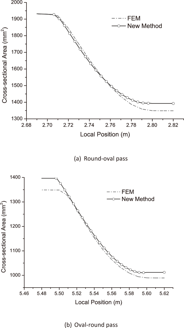
Comparison of calculated CSA from the new method with FEM simulation.

Figure 5 shows the comparison between calculated temperatures by the new method and the simulated results by FEM. It is evident that there is a good agreement between them at corresponding positions, except for some subtle differences in transient state. In the rolling stage, the main difference is caused by the calculation of temperature rise. On the one hand, the generated heat is influenced by the plastic deformation and friction parameters, such as strain and heat convert fraction of strain-rate energy and friction coefficient etc., it is difficult to maintain the same values of them between the two methods for all time. On the other hand, the FEM considers the produced heat as the average thermal load for unit volume of each element, and the method in this paper considers it as the average thermal load of the whole cross-section, it may lead to the transient difference between them at specific positions. In the stage between passes, the main difference is caused by the different pass time which is determined by the difference of calculated workpiece speeds. So, the industrial process data, such as rolling power and workpiece speeds etc., were used to correct the parameters.

Fig. 5.

Calculated temperatures of the two passes as compared with FEM simulated results.

4.2. Compared with the Industrial Measured Data

It is difficult to measure the actual surface profiles of workpiece on-line during rolling, so the elongations were calculated for the comparison between the new method and practice results. In Fig. 6, the coefficients of elongation solved by the improved formulas are compared with the results calculated from industrial measured rolling speeds. As can be seen, all the calculated results from the new method are in good agreement with the corresponding practice values.

Fig. 6.

Comparison of calculated coefficient of elongation with practice.

The predicted temperature profiles of workpiece successively evaluated from the furnace entrance to the coil collecting station and its comparison with the measured surface temperatures are shown in Fig. 7. Most of the variances (errors) between calculated and measured surface temperatures are within the range of standard deviation. In conclusion, the new method is suitable enough for engineering application.

Fig. 7.

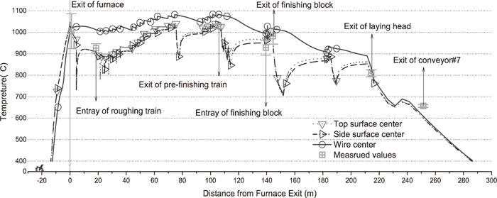
Calculated time-temperature history of a workpiece during the whole hot-rolling process.

5. Conclusion

In this paper, a new 2D numerical method has been developed for calculating the temperature distribution of rod during multi-pass hot rolling. A simple grid remesh algorithm with the improved surface profile determination formulas was proposed to deal with the deformation of workpiece during rolling based on the energy rate balance of the control volume. The calculation of each step is very quick without solving the constitutive equation by iterative method. The areas (elongations) and temperature profiles of the cross-section predicted by the new method are in agreement with those obtained from FEM simulation and industrial measurement. The proposed method might potentially be a valuable tool for the on-line temperature control and quality prediction.

Acknowledgements

This work was supported by the National Key Basic Research and Development Program of China (2009CB320602) and the National Natural Science Foundation of China (61025018). The authors are grateful to Xingtai Iron & Steel Corp., LTD, China for providing technical supports and industrial data.

References

• 1)   H.-C.  Kwon and  Y.-T.  Im: J. Mater. Process. Technol., 167 (2005), 273.
• 2)   Y.  Lee,  S.  Choi and  P. D.  Hodgson: J. Mater. Process. Technol., 125 (2002), 678.
• 3)   S. V.  Patankar: Numerical heat transfer and fluid flow. Hemisphere Publishing Corp, London, England, (1980).
• 4)   T.  Shinokura and  K.  Takai: J. Appl. Metalwork, 2 (1982), 94.
• 5)   Y.  Lee,  S.  Choi and  Y. H.  Kim: J. Mater. Process. Technol., 108 (2000), 87.
• 6)   S. C.  Chapra and  R. P.  Canale: Numerical Methods for Engineers. McGraw-Hill, New York, US, (2000).