Analysis of Diffusion-controlled Phenomena at the Interface of α/γ Diffusion Couples of Stainless Steels

Abstract

The interdiffusion of Ni, Cr, and Mo across the interface in the diffusion couples of type444/type316L stainless steels was simulated using the DICTRA software. The distance of interface migration and the Ni diffusion distance into the ferrite phase were calculated and compared with the experimental results previously reported by a present author. The calculated results agree very well with the experimental results. An analytical model based on the analytical solutions for the semi-infinite solute diffusion equations has been proposed. In the model, all solute elements are considered and diffusion paths are calculated. The supersaturations of the solutes defined both for the ferrite phase and the austenite phase are calculated from the calculated diffusion paths. According to the model it is shown that the temperature dependency of the interface migration distance and the Ni diffusion distance can be quantitatively evaluated by the supersaturation for Ni.

1. Introduction

The interdiffusion across interfaces plays important roles in not only bonding of dissimilar materials but also precipitations and phase transformations in manufacturing and welding processes of practical complex alloys, such as stainless steels. A present author previously reported on the bonding experiment of the diffusion couple using ferritic stainless steel type444 and austenitic stainless steel type316L.¹⁾ Diffusion couples can be used to study interdiffusion phenomena at the interface other than to determine the isothermal phase diagram. Owing to their simplicity, diffusion couples may serve as a simple physical model for the interface in industrial materials.

Simulation methods are very useful tools to investigate complex phenomena at interfaces of industrial materials. The interfaces may be modeled in detail by sharp interface methods such as DICTRA.^2,3) These simulation models can be applied to multicomponent and multiphase systems and can describe complex behaviors exhibited by the interfaces of materials.^4,5,6,7,8) These simulations are based on numerical calculations of full diffusion fields or diffusion paths.

Simple analytical models^{9,10,11,12,13)} are also quite useful to interpret the results of simulations and experiments and to understand the underlying physical phenomena. Moreover, the simulation methods may be quite time consuming. This study aims to establish a simple analytical model that can predict diffusion paths for multicomponent systems. Kajihara et al.¹¹⁾ calculated diffusion paths using approximate solutions of the diffusion equations for the semi-infinite α/γ diffusion couples of ternary Fe–Cr–Ni systems. Here we propose a model that is applicable to general systems that have N solute elements. To obtain a local equilibrium and calculate the diffusion paths, the operating tie line at the interface must be determined. In general, for multicomponent alloys, the local equilibrium at the phase interface has to be numerically determined by seeking a common growth rate for all independent components. Therefore, calculating the local equilibrium at interfaces needs complex numerical procedures. The present analytical model is based on analytical solutions of semi-infinite one-dimensional diffusion equations for all solute elements. The migration of the α/γ interface is described by the equations derived from flux balance conditions. We present a procedure for calculating the local equilibrium solute concentrations at the α/γ interface and the diffusion paths. The migration distance of the interface is also calculated as a function of time.

In an experimental investigation conducted by a present author, couples of type444 and type316L stainless steels annealed for solution treatment were heated for diffusion bonding using a high frequency induction heater in 99.9% argon gas at various holding temperatures and holding time. In the experiment, the distance of interface migration was measured at the temperatures of 1373, 1473, and 1523 K for up to 1000 s. Concentration profiles were also measured along the direction normal to the moving ferrite (α-phase)/austenite (γ-phase) interface by standard electron probe microanalysis (EPMA). In the bonding process, the γ-phase was transformed to the α-phase at the interface by solute diffusion from the γ-phase into the α-phase, and consequently, the interface migrated to the γ-phase side. In the present study, the simulations of multicomponent diffusion in the diffusion couples of type444/type316L stainless steels have been carried out using the DICTRA software and compared with the experimental results. In the simulation, Fe–Cr–Ni–Mo quaternary model alloys are considered. The compositions of the model alloys and the simulation conditions correspond to the experiments. The distance of interface migration and the nickel diffusion distance into the α-phase have been calculated using the DICTRA and compared with the experimental results. The experimental and simulation results are analyzed by the present analytical model. The present model is applicable to more general systems which have N solute elements.

2. DICTRA Simulation Procedures

The simulations were performed using the DICTRA software, which is a software package used for the simulation of diffusion-controlled transformations in multicomponent alloy systems having a simple geometry such as diffusion couples. Therefore, the DICTRA software is thought to be suitable for the present simulations.

In the simulations, the Cr–Ni–Mo–Fe quaternary system is considered. The compositions of the present model alloys are listed in Table 1. The compositions are chosen on the basis of a previous experimental investigation.¹⁾ The DICTRA simulations were based on numerical solutions of multicomponent diffusion equations using kinetic and thermodynamic databases, assuming a local equilibrium at the moving interface. A local equilibrium at the moving interface is established on the basis of flux balances of solutes through the interface.

Table 1. Chemical compositions of the model alloys used (mass%).

	Cr	Ni	Mo	Fe
Type444 (α)	19	0	2	Bal.
Type316L (γ)	17	12	2	Bal.

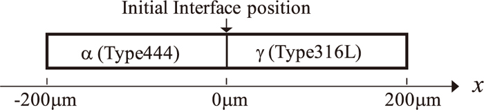
In the diffusion couple system investigated, the interface was observed to be planar. The model for the simulation is shown in Fig. 1. In this setup, a one-dimensional model consisting of a ferrite matrix (α-phase, type444 stainless steel) and an austenite matrix (γ-phase, type316L stainless steel) with a length of 200 μm is considered. This length is sufficient for simulation because the diffusion distance is less than 200 μm, as can be seen below. The version of DICTRA used is 26. The thermodynamic and kinetic databases used were the TCFe6 and the MOBFe1, respectively.

Fig. 1.

Computational model for the DICTRA simulations.

In DICTRA simulations, cross diffusion of all elements is considered. It is thus concluded that the present approach should be suitable as an engineering tool to study diffusion interactions of multicomponent systems.

The simulations were performed at 1373, 1473, and 1523 K up to 1000 s corresponding to the experiments. The initial solute concentration profiles of the α- and γ-phases are set to be the bulk compositions of the model alloys for type444 and type316L stainless steels. The solute concentration profiles and the interface positions were calculated at each temperature. The nickel diffusion distances were calculated using the nickel concentration profiles.

3. Simulation Results

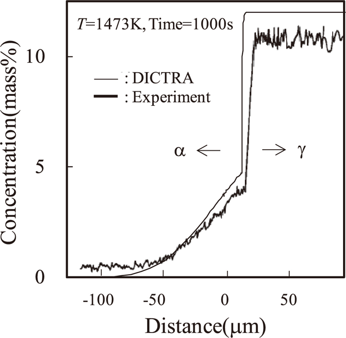
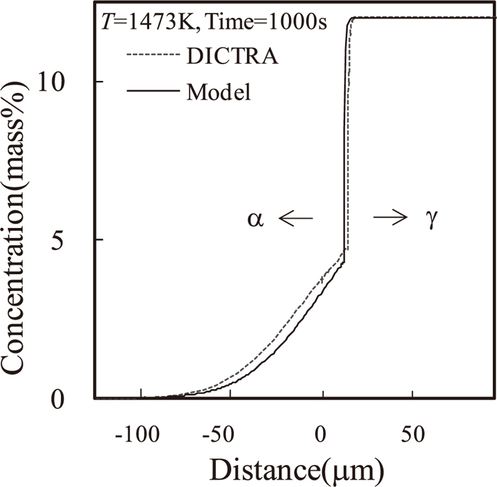
Figure 2 shows the calculated temporal evolution of the solute concentration profiles after 100, 500, and 1000 s in the diffusion couple at 1523 K. The origin of the distance is the initial interface position. The position of the discontinuity seen in the concentration profile corresponds to the position of the interface. The migration distance is denoted as δ(t) in Fig. 2. Λ(t) is defined as the nickel diffusion distance as a function of time. This value is calculated as the width of the region in the α-phase, where the nickel concentration is more than 1%. It is shown that nickel deeply diffuses into the α-phase compared with chromium and molybdenum atoms, and the interface between α- and γ-phases moves to the γ-phase side with time. The concentrations of solutes in the regions near the left and right boundaries approach the bulk concentration of α- and γ-phases, respectively. This means that the length of 200 μm for each phase is sufficient for the simulation. Figure 3 shows the simulation result of nickel diffusion profiles in the vicinity of the α/γ interface, together with the EPMA measurement at 1473 K after 1000 s. The agreement between the calculated and the experimental values is satisfactory.

Fig. 2.

Time evolution of the solute concentration profiles at 1523 K. The origin of the distance is the initial interface position.

Fig. 3.

Nickel diffusion profiles in the vicinity of the α/γ interface obtained from the DICTRA simulation at 1473 K after 1000 s, together with the EPMA measurement. The result obtained by the simulation is indicated by a solid line and the experimental result is indicated by a fluctuating solid line.

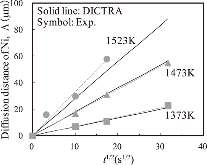
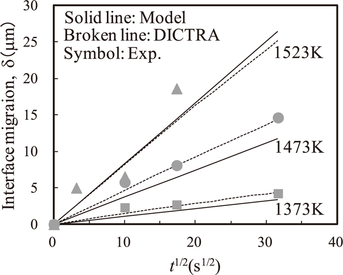
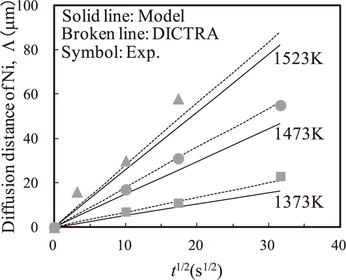
Figures 4 and 5 show the calculated δ and Λ versus the square root of the holding time indicated by solid lines, together with the experimental data indicated by symbols, respectively. Both δ and Λ approximately increase in proportion to the square root of the holding time.   

$$\delta \left(t\right)=m_{\delta }\left(T\right)\sqrt{t}\hspace{0.17em}\hspace{0.17em},\hspace{0.17em}\hspace{0.17em}\mathrm{\Lambda }\left(t\right)=m_{\mathrm{\Lambda }}\left(T\right)\sqrt{t},$$(1)

where m_δ(T) and m_Λ(T) are coefficients depending on the temperature. This means that the reaction is diffusion controlled and stays at a steady state during the process. The simulation results agree quantitatively very well with the experimental results. Especially, the differences between the experimental and the simulation results at 1373 and 1473 K are very small.

Fig. 4.

Interface migration distance δ at each temperature as a function of the square root of the holding time at 1373, 1473, and 1523 K. Solid lines denote the DICTRA simulation results, and symbols and broken lines denote the experimental results.

Fig. 5.

Nickel diffusion distance Λ at 1373, 1473, and 1523 K as a function of the square root of the holding time. Solid lines denote the DICTRA simulation results and Symbols and broken lines denote the experimental results.

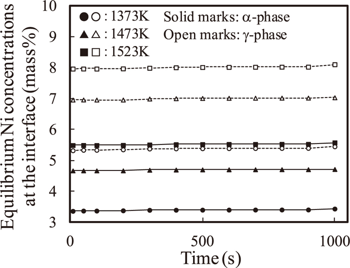
Figure 6 shows the local equilibrium concentrations of nickel versus the holding time at 1373, 1473, and 1523 K. The local equilibrium concentrations for α- and γ-phases are almost constant during the process. This means that the local equilibrium is established soon after the simulation has started, and the concentration values are constant during the simulation.

Fig. 6.

Temporal evolutions of the local equilibrium concentrations of nickel with the holding time at 1373, 1473, and 1523 K from the DICTRA simulations.

4. Analytical Model

4.1. Analytical Solutions for Solute Diffusion Equations

We propose a simple analytical model describing interface migration induced by solute diffusion in the present diffusion couple system. Figure 6 shows that the present system is in a steady state during the process; thus, we construct a model on the basis of steady state solutions of solute diffusion equations. Here all solutes must be considered for the flux balance at the interface. Thus, in the analysis below, we do not restrict particular elements. Solute diffusion in the diffusion couples is described by the following one-dimensional equation of diffusion.   

$$\frac{\partial c}{\partial t}=\frac{\partial }{\partial x}\left(D\frac{\partial c}{\partial x}\right)\hspace{0.17em}\hspace{0.17em},\hspace{0.17em}\hspace{0.17em}\hspace{0.17em}\left(D=D_{\alpha }\hspace{0.17em}\hspace{0.17em}\left(x<\delta \right)\hspace{0.17em}\hspace{0.17em},\hspace{0.17em}\hspace{0.17em}\hspace{0.17em}D=D_{\gamma }\hspace{0.17em}\hspace{0.17em}\left(x>\delta \right)\right)\hspace{0.17em}\hspace{0.17em}$$(2)

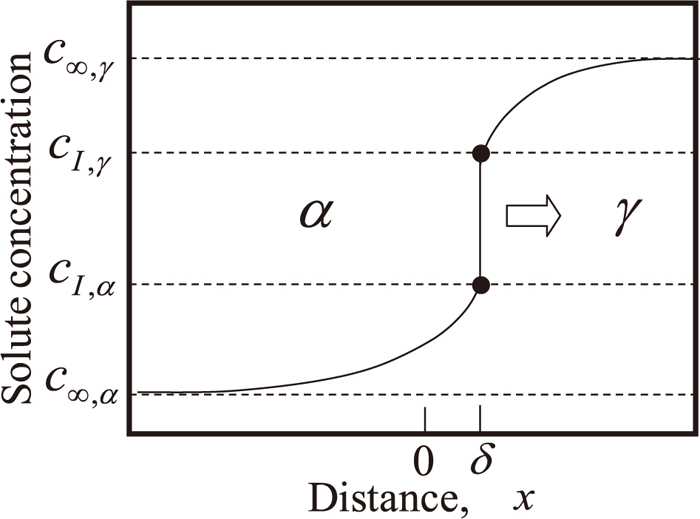
where δ is the interface position and D_α and D_γ are the solute diffusion coefficients in α- and γ-phases, respectively. In the model, the cross-terms in diffusion equations were ignored.¹¹⁾ The diffusion of interstitial elements is affected by the composition of alloys. Therefore, the cross terms cannot be ignored for interstitial elements. In the model, only substitutional elements are considered. As an example of the concentration profiles of a solute, the nickel concentration profile across the α/γ interface with the boundary conditions is schematically depicted in Fig. 7. In this figure, the distance x is measured from the initial position of the α/γ interface. The local equilibrium concentrations for α- and γ-phases are denoted by c_I,α and c_I,γ, respectively. c_∞,α and c_∞,γ are the bulk concentrations for α- and γ-phases, respectively. This system is assumed to be infinite for the directions to the α and γ bulks. In the diffusion couples considered here, the interface is isolated. Therefore, this assumption is reasonable. Equation (2) with the boundary conditions shown in Fig. 2 has its analytical solution as follows.   

$$c\left(\eta \right)=c_{\infty ,\alpha }+\left(c_{I,\alpha }-c_{\infty ,\alpha }\right)\frac{1+\mathrm{e}\mathrm{r}\mathrm{f}\left(\eta /2\sqrt{D_{\alpha }}\right)}{1+\mathrm{e}\mathrm{r}\mathrm{f}\left(\alpha /2\sqrt{D_{\alpha }}\right)}\mathrm{\hspace{0.17em} }\mathrm{\hspace{0.17em} }\left(\eta <\alpha \hspace{0.17em}\hspace{0.17em}\hspace{0.17em}\left(x<\delta \right)\right),$$(3a)

and   

$$c\left(\eta \right)=c_{\infty ,\gamma }+\left(c_{I,\gamma }-c_{\infty ,\gamma }\right)\frac{1-\mathrm{e}\mathrm{r}\mathrm{f}\left(\eta /2\sqrt{D_{\gamma }}\right)}{1-\mathrm{e}\mathrm{r}\mathrm{f}\left(\alpha /2\sqrt{D_{\gamma }}\right)}\mathrm{\hspace{0.17em} }\mathrm{\hspace{0.17em} }\left(\eta >\alpha \hspace{0.17em}\hspace{0.17em}\hspace{0.17em}\left(x>\delta \right)\right),$$(3b)

where $\eta \equiv x/\sqrt{t}$ , $\alpha \equiv \delta /\sqrt{t}$ .

Fig. 7.

Schematic illustration of the local equilibrium profile of nickel at the interface.

The flux balance for the solute at the interface gives the following equation including the migration rate dδ/dt.¹⁰⁾   

$$\left(c_{I,\gamma }-c_{I,\alpha }\right)\frac{d\delta }{dt}=D{{}_{\alpha }\frac{\partial c}{\partial x}|}_{\delta -}-D{{}_{\gamma }\frac{\partial c}{\partial x}|}_{\delta +}\hspace{0.17em}\hspace{0.17em}\hspace{0.17em}.$$(4)

The analytical solution (Eq. (3)) with the above flux balance condition yields the following equation   

$$\delta =\left({\mathrm{\Omega }}_{\alpha }\sqrt{D_{\alpha }}\frac{\mathrm{e}\mathrm{x}\mathrm{p}\left(-{\lambda }_{\alpha }^2\right)}{1+\mathrm{e}\mathrm{r}\mathrm{f}\left({\lambda }_{\alpha }\right)}-{\mathrm{\Omega }}_{\gamma }\sqrt{D_{\gamma }}\frac{\mathrm{e}\mathrm{x}\mathrm{p}\left(-{\lambda }_{\gamma }^2\right)}{1-\mathrm{e}\mathrm{r}\mathrm{f}\left({\lambda }_{\gamma }\right)}\right)\frac{2\sqrt{t}}{\sqrt{\pi }}\mathrm{\hspace{0.17em} },$$(5)

where the following dimensionless proportionally coefficients are defined.   

$${\lambda }_{\alpha }\equiv \alpha /2\sqrt{D_{\alpha }}=\delta /2\sqrt{D_{\alpha }t}\hspace{0.17em}\hspace{0.17em},\hspace{0.17em}\hspace{0.17em}\hspace{0.17em}\hspace{0.17em}{\lambda }_{\gamma }\equiv \alpha /2\sqrt{D_{\gamma }}=\delta /2\sqrt{D_{\gamma }t}\hspace{0.17em}\hspace{0.17em}.$$(6)

λ_α and λ_γ are related each other as follows.   

$${\lambda }_{\gamma }={\lambda }_{\alpha }\sqrt{\frac{D_{\alpha }}{D_{\gamma }}}.$$(7)

Ω_α and Ω_γ in Eq. (5) are supersaturations of the solute for α- and γ-phases respectively, which are defined as follows.   

$${\mathrm{\Omega }}_{\alpha }\equiv \frac{c_{I,\alpha }-c_{\infty ,\alpha }}{c_{I,\gamma }-c_{I,\alpha }}\hspace{0.17em}\hspace{0.17em},\hspace{0.17em}\hspace{0.17em}\hspace{0.17em}\hspace{0.17em}{\mathrm{\Omega }}_{\gamma }\equiv \frac{c_{\infty ,\gamma }-c_{I,\gamma }}{c_{I,\gamma }-c_{I,\alpha }}\hspace{0.17em}\hspace{0.17em}.$$(8)

Equation (5) implies that the migration distance δ is proportional to square root of time. Finally the following equation for λ_α is obtained.   

$$\sqrt{\pi }={\mathrm{\Omega }}_{\alpha }{\lambda }_{\alpha }^{-1}\frac{\mathrm{e}\mathrm{x}\mathrm{p}\left(-{\lambda }_{\alpha }^2\right)}{1+\mathrm{e}\mathrm{r}\mathrm{f}\left({\lambda }_{\alpha }\right)}-{\mathrm{\Omega }}_{\gamma }{\lambda }_{\alpha }^{-1}\sqrt{\frac{D_{\gamma }}{D_{\alpha }}}\frac{\mathrm{e}\mathrm{x}\mathrm{p}\left(-{\lambda }_{\alpha }^2{D}_{\alpha }/D_{\gamma }\right)}{1-\mathrm{e}\mathrm{r}\mathrm{f}\left({\lambda }_{\alpha }\sqrt{D_{\alpha }/D_{\gamma }}\right)}\mathrm{\hspace{0.17em} }.$$(9)

Equation (9) is usually solved numerically. From the obtained values of λ_α andλ_γ, the migration distance of the interface is calculated using the equations below.   

$$\delta \left(t\right)=2{\lambda }_{\alpha }\sqrt{D_{\alpha }t}=2{\lambda }_{\gamma }\sqrt{D_{\gamma }t}\hspace{0.17em}\hspace{0.17em}.$$(10)

λ_α and λ_γ are functions of the local equilibrium concentrations at the interface through Eq. (8).

The nickel diffusion distance can be obtained from Eq. (3a). The nickel diffusion distance is defined as the width of the α-phase region, where the nickel concentration is more than c₁(=1 mass%). The following dimensionless coefficient is also defined.   

$$x_1=2{\xi }_1\sqrt{D_{\alpha }t}\hspace{0.17em}\hspace{0.17em}.$$(11)

Here x₁ is defined as the x-coordinate where the concentration value is c₁. When λ_α is substituted in Eq. (3a), the following relation is obtained.   

$$c_1=c_{\infty ,\alpha }+\left(c_{I,\alpha }-c_{\infty ,\alpha }\right)\frac{1+\mathrm{e}\mathrm{r}\mathrm{f}\left({\xi }_1\right)}{1+\mathrm{e}\mathrm{r}\mathrm{f}\left({\lambda }_{\alpha }\right)}\hspace{0.17em}\hspace{0.17em}.$$(12)

The ξ₁ is calculated by numerically solving Eq. (12). The nickel diffusion distance Λ is calculated as follows.   

$$\begin{array}{l}\mathrm{\Lambda }=\delta +\left|x_1\right|=2{\lambda }_{\alpha }\sqrt{D_{\alpha }t}-2{\xi }_1\sqrt{D_{\alpha }t}\\ =2\left({\lambda }_{\alpha }-{\xi }_1\right)\sqrt{D_{\alpha }t}=2{\lambda }_{\mathrm{\Lambda }}\sqrt{D_{\alpha }t}\end{array}\hspace{0.17em}\hspace{0.17em},$$(13)

where λ_Λ = λ_α – ξ₁. Equation (13) implies that Λ obeys the parabolic growth rule as well as δ.

4.2. Approximate Expression for the Interface Migration Distance

Equation (9) is usually solved numerically to obtain λ_α as mentioned above. Here we derive an analytical expression for λ_α. For error function, there are following two approximate relations.   

$$\text{erf}\left(z\right)\approx \frac{2}{\sqrt{\pi }}z\hspace{0.17em},\hspace{0.17em}\hspace{0.17em}\hspace{0.17em}\hspace{0.17em}\hspace{0.17em}\hspace{0.17em}\hspace{0.17em}\text{for}\hspace{0.17em}\hspace{0.17em}\hspace{0.17em}z<\hspace{0.17em}1,$$(14)

and   

$$\mathrm{e}\mathrm{r}\mathrm{f}\left(z\right)\approx 1-\frac{1}{\sqrt{\pi }z}exp\left(-z^2\right)\hspace{0.17em},\hspace{0.17em}\hspace{0.17em}\hspace{0.17em}\hspace{0.17em}\hspace{0.17em}\hspace{0.17em}\hspace{0.17em}\text{for}\hspace{0.17em}\hspace{0.17em}\hspace{0.17em}z\hspace{0.17em}>\hspace{0.17em}1.$$(15)

As can be seen later, the values of λ_α is less than 1 and $\sqrt{D_{\gamma }/D_{\alpha }}$ is smaller than 0.1. This implies that Eqs. (14) and (15) can be used in the present case.

The equation below is also used.   

$$exp\left(z^2\right)\approx 1+z^2\approx 1,\hspace{0.17em}\hspace{0.17em}\hspace{0.17em}\hspace{0.17em}\hspace{0.17em}\hspace{0.17em}\hspace{0.17em}\hspace{0.17em}\text{for}\hspace{0.17em}\hspace{0.17em}\hspace{0.17em}z<\hspace{0.17em}1\hspace{0.17em}\hspace{0.17em}.$$(16)

The right hand side of Eq. (9) can be approximated using above three relations.   

$$\text{The}\hspace{0.17em}\text{first}\hspace{0.17em}\text{term}\approx {\mathrm{\Omega }}_{\alpha }{\lambda }_{\alpha }^{-1}\frac{1}{1+\frac{2}{\sqrt{\pi }}{\lambda }_{\alpha }}=\frac{{\mathrm{\Omega }}_{\alpha }}{{\lambda }_{\alpha }+\frac{2}{\sqrt{\pi }}{\lambda }_{\alpha }^2}\hspace{0.17em}\hspace{0.17em},$$(17)

and   

$$\text{The}\hspace{0.17em}\text{second}\hspace{0.17em}\text{term}\approx -{\mathrm{\Omega }}_{\gamma }{\lambda }_{\gamma }^{-1}\frac{\mathrm{e}\mathrm{x}\mathrm{p}\left(-{\lambda }_{\gamma }^2\right)}{\frac{1}{\sqrt{\pi }{\lambda }_{\gamma }}\mathrm{e}\mathrm{x}\mathrm{p}\left(-{\lambda }_{\gamma }^2\right)}=-\sqrt{\pi }{\mathrm{\Omega }}_{\gamma }\hspace{0.17em}\hspace{0.17em}.$$(18)

Substituting Eqs. (17) and (18) into Eq. (9), the following quadratic equation is obtained.   

$${\lambda }_{\alpha }^2+\frac{\sqrt{\pi }}{2}{\lambda }_{\alpha }-\frac{{\mathrm{\Omega }}_{\alpha }}{2\left(1+{\mathrm{\Omega }}_{\gamma }\right)}=0\hspace{0.17em}\hspace{0.17em}.$$(19)

By solving Eq. (19), the following solution for λ_α is obtained.   

$${\lambda }_{\alpha }=\frac{\sqrt{\pi }}{4}\left(\sqrt{1+\frac{8}{\pi }\cdot \frac{{\mathrm{\Omega }}_{\alpha }}{1+{\mathrm{\Omega }}_{\gamma }}}-1\right)\hspace{0.17em}\hspace{0.17em}.$$(20)

Using Eqs. (10) and (20), the interface migration distance δ(t) can be expressed as a function of the supersaturations Ω_α and Ω_γ as follows.   

$$\delta \left(t\right)=\frac{\sqrt{\pi }}{2}\left(\sqrt{1+\frac{8}{\pi }\cdot \frac{{\mathrm{\Omega }}_{\alpha }}{1+{\mathrm{\Omega }}_{\gamma }}}-1\right)\hspace{0.17em}\sqrt{D_{\alpha }t}\hspace{0.17em}\hspace{0.17em}.\hspace{0.17em}$$(21)

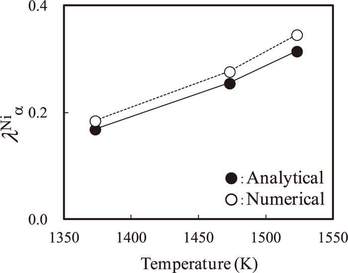
We examine the validity of the approximate solution for λ_α given by Eq. (20) using the DICTRA simulation results at 1373, 1473, and 1523 K. The numerical solution for Eq. (9) and the approximate solution given by Eq. (20) using Ω_α and Ω_γ calculated from the time average for 1–1000 s of the local equilibrium concentrations for α- and γ-phases at the interface are compared in Fig. 8. The agreement between them is fairly good, and the validity of the approximate solution for λ_α given by Eq. (20) is demonstrated. This analytical expression is used for the analysis below.

Fig. 8.

Comparison of λ_α obtained by numerically solving Eq. (9) and obtained by using the approximate solution Eq. (20) for parameters Ω_α and Ω_γ calculated from the local equilibrium concentration of nickel from the DITRA simulation results.

4.3. Calculation of the Local Equilibrium Concentrations at the Interface

In the following analysis, we formulate the procedure to calculate the local equilibrium concentrations of the solutes and the interface migration distance δ (t) using the approximate expression for λ_α. Iron is regarded as a solvent and nickel, chromium, and molybdenum are regarded as solutes in the following. For a while, we do not restrict Fe–Cr–Ni–Mo quaternary systems, but the number of solutes is set to N for generalization of the present model. Thus, the number of all elements is N+1, including the solvent. The migration distance of the α/γ interface is expressed by the following equation for each element using Eq. (10).   

$${\delta }_j\left(t\right)=2{\lambda }_{\alpha }^j\sqrt{D_{\alpha }^{j}t}\hspace{0.17em}\hspace{0.17em}\hspace{0.17em}\hspace{0.17em}\left(j=1,\cdots ,N\right).$$(22)

The migration distances calculated for each element must be equal to each other independently; thus, the following relations hold.¹¹⁾   

$${\delta }_{\text{1}}\left(t\right)={\delta }_{\text{2}}\left(t\right)=\cdots ={\delta }_N\left(t\right).$$(23)

Each δ (t) is a function of the local equilibrium concentrations at the interface. If each δ(t) is explicitly expressed by the local equilibrium solute concentrations, Eq. (23) gives N-1 equations for 2N unknown concentrations. To obtain local equilibrium solute concentrations, N+1 additional equations are necessary. The equilibrium concentration at α- and γ-phases must be connected by tie lines.¹¹⁾ However, it is difficult to determine the whole α/γ tie lines in the solute concentration space. Therefore, we assume the approximate relation $c_{I,\gamma }^j=k_{\gamma /\alpha }^j{c}_{I,\alpha }^j$ , which is usually used for dilute solutions. In the present case, we have to consider the solvent as well as the solutes because the present systems are not dilute solutions, and the concentrations of the solvent and solutes are comparable. Thus, we assume the following relations for thermal equilibrium.   

$$c_{I,\gamma }^j=k_{\gamma /\alpha }^j{c}_{I,\alpha }^j\hspace{0.17em}\hspace{0.17em}\left(j=1,\cdots ,N+1\right)\hspace{0.17em}.$$(24)

Here the solvent is included. Thus, there are N+1 additional equations for the solute concentrations available. The solvent concentrations in α- and γ-phases can be expressed by all the solute concentrations. Thus, the number of unknowns remains 2N. Finally, 2N equations for 2N unknowns have been obtained. It is possible to solve 2N equations (Eqs. (23) and (24)) and obtain the 2N local equilibrium solute concentrations at the interface.

5. Results and Discussion

Here we apply the analytical model to the present Fe–Cr–Ni–Mo quaternary system. From Eqs. (22) and (23), the following equations for nickel, chromium, and molybdenum are obtained.   

$${\lambda }_{\alpha }^{\text{Ni}}\sqrt{D_{\alpha }^{\text{Ni}}}={\lambda }_{\alpha }^{\text{Cr}}\sqrt{D_{\alpha }^{\text{Cr}}}\hspace{0.17em},\hspace{0.17em}\hspace{0.17em}{\lambda }_{\alpha }^{\text{Ni}}\sqrt{D_{\alpha }^{\text{Ni}}}={\lambda }_{\alpha }^{\text{Mo}}\sqrt{D_{\alpha }^{\text{Mo}}}.$$(25)

In addition to the above equations, the equilibrium conditions are given as follows.   

$$c_{I,\gamma }^j=k_{\gamma /\alpha }^j{c}_{I,\alpha }^j\hspace{0.17em}\hspace{0.17em}\left(j=\text{Ni,Cr,Mo,Fe}\right),$$(26)

where the local equilibrium concentrations for the solvent, iron, are calculated by the sums of the concentrations of all solutes.

The coefficients ${\lambda }_{\alpha }^j$ ’s are expressed by Eq. (20); thus, they are functions of $c_{I,\alpha }^j$ and $c_{I,\gamma }^j$ through ${\mathrm{\Omega }}_{\alpha }^j$ and ${\mathrm{\Omega }}_{\gamma }^j$ . We obtained six equations (Eqs. (25) and (26)) for six unknowns, $c_{I,\alpha }^{\text{Ni}}$ , $c_{I,\gamma }^{\text{Ni}}$ , $c_{I,\alpha }^{\text{Cr}}$ , $c_{I,\gamma }^{\text{Cr}}$ , $c_{I,\alpha }^{\text{Mo}}$ , and $c_{I,\gamma }^{\text{Mo}}$ . These equations can be solved numerically. The equilibrium distribution coefficients of nickel, chromium and molybdenum between α/γ phases for 1373, 1473, and 1523 K were calculated using Thermo-Calc.^3,14) The calculations were performed using the model alloys listed in Table 1. Actually, the compositions at the interface are different from the bulk compositions. However, it is almost impossible to calculate the equilibrium distribution coefficients for the exact compositions at the interface before obtaining them. The calculated equilibrium distribution coefficients for each temperature are listed in Table 2. The diagonal elements of the diffusion matrix at each temperature for the solutes in α- and γ- phases are extracted from the DICTRA database (MOBFe1). They are also listed in Table 2.

Table 2. Thermodynamics data used (Diffusion coefficients in m²/s).

T	Ni			Cr			Mo			Fe
(K)	kγ/α	Dα	Dγ	kγ/α	Dα	Dγ	kγ/α	Dα	Dγ	kγ/α
1373	1.63	1.25×10–13	8.94×10–16	0.78	2.33×10–13	2.22×10–15	0.63	1.91×10–13	2.63×10–15	1.04
1473	1.51	5.66×10–13	5.04×10–15	0.80	8.92×10–13	1.23×10–14	0.62	6.34×10–13	1.09×10–14	1.03
1523	1.45	1.10×10–12	1.10×10–14	0.81	1.62×10–12	2.66×10–14	0.62	1.08×10–12	2.08×10–14	1.02

Equations (25) and (26) were numerically solved to obtain the local equilibrium compositions at the interface. The diffusion paths were calculated using the local equilibrium compositions and Eq. (3). In Fig. 9, the diffusion paths calculated using the present model are plotted with the diffusion paths obtained from the DICTRA simulations for 1373, 1473, and 1523 K after 1000 s on the Ni–Cr concentration plane. The diffusion paths for the model and the DICTRA are denoted by solid and broken lines, respectively. The local equilibrium concentrations of nickel and chromium calculated by the model and the DICTRA are denoted by solid circles and open circles, respectively. The bulk concentrations are denoted by solid triangles. The calculated diffusion paths are close to the diffusion paths obtained by the DICTRA simulation for three temperatures.

Fig. 9.

Diffusion paths and local equilibrium compositions at the interface calculated by the model and the DICTRA simulation at (a) 1373 K, (b) 1473 K, and (c) 1523 K after 1000 s. The diffusion paths are plotted on the Ni–Cr concentration plane. The solid and broken lines denote the calculated results by the model and the DICTRA, respectively. The local equilibrium concentrations of nickel and chromium calculated by the model and the DICTRA are denoted by solid and open circles, respectively. The bulk concentrations are shown by solid triangles. The two grey lines are the equilibrium concentrations of α- and γ-phases in Ni–Cr space. The numbers beside these lines are the local equilibrium concentrations of molybdenum.

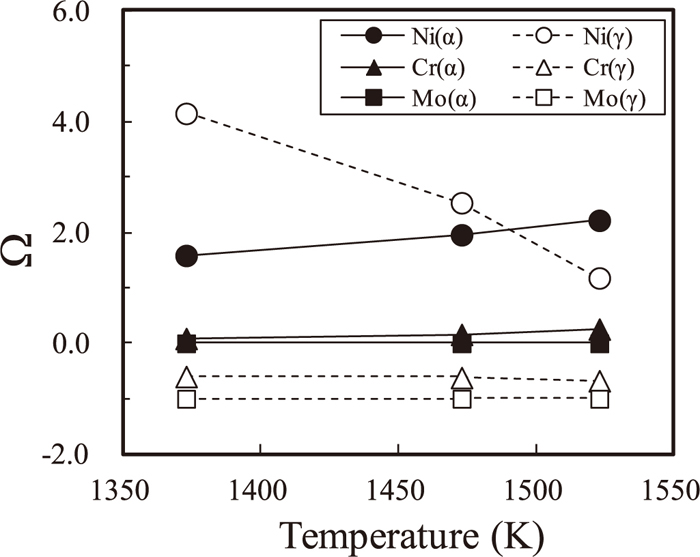
The values of the supersaturations are calculated by the local equilibrium concentrations at the interface using the present model. Figure 10 shows the supersaturations for α- and γ-phases versus the temperatures. The values of the supersaturations ${\mathrm{\Omega }}_{\alpha }^j$ and ${\mathrm{\Omega }}_{\gamma }^j$ can be negative by the definition given by Eq. (8). The absolute values of the supersaturations are more valid than the values themselves from the view of the driving force for phase transformation. 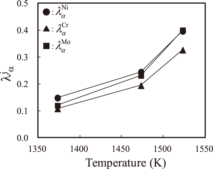This figure shows that as the increase of the temperature, ${\mathrm{\Omega }}_{\gamma }^{\text{Ni}}$ decreases and ${\mathrm{\Omega }}_{\alpha }^{\text{Ni}}$ increases, while the other supersaturations, ${\mathrm{\Omega }}_{\alpha }^{\text{Cr}}$ , ${\mathrm{\Omega }}_{\gamma }^{\text{Cr}}$ , ${\mathrm{\Omega }}_{\alpha }^{\text{Mo}}$ and ${\mathrm{\Omega }}_{\gamma }^{\text{Mo}}$ remain almost constant. This means that the driving force for phase transformation at the interface is increased by the nickel diffusion from the γ-phase to the α-phase. The coefficients ${\lambda }_{\alpha }^j$ ’s calculated using ${\mathrm{\Omega }}_{\alpha }^j$ ’s and ${\mathrm{\Omega }}_{\gamma }^j$ ’s as a function of the temperature are shown in Fig. 11. 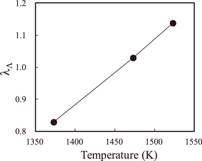The figure shows that ${\lambda }_{\alpha }^j$ ’s for nickel, chromium, and molybdenum increase with temperature. Figure 12 shows λ_Λ versus the temperature. The λ_Λ increases with temperature. From the temperature dependency of ${\lambda }_{\alpha }^j$ ’s and λ_Λ, it is concluded that the migration distance of the interface δ and the nickel diffusion distance Λ increase with temperature through not only the diffusion coefficients of the solutes in the α-phase but also ${\lambda }_{\alpha }^j$ ’s and λ_Λ . This implies that the increase in δ and Λ is enhanced by the increase of the driving force for the transformation of the γ-phase to the α-phase. Figure 13 compares δ calculated by the present model with δ obtained from the DICTRA simulation as a function of the square root of the holding time, together with experimental results. The results calculated by the model denoted by the solid lines agree very well with the DICTRA simulation results denoted by the broken lines, especially for 1523 K. Figure 14 compares Λ calculated from the present model with Λ from the DICTRA simulation as a function of the square root of the holding time, together with the experimental results. The agreement between the results from the model and the simulations is good. Figure 15 shows the nickel diffusion profile calculated using the model and the simulation. The above good agreements between the model and the DICTRA simulation results demonstrate that the model is sufficient for describing the diffusion-controlled phenomena observed in the α/γ interface of the diffusion couples.

Fig. 10.

Supersaturations of the nickel, chromium and molybdenum defined for α- and γ-phases versus temperature. The values were calculated from the local equilibrium compositions at the interface obtained by the present model.

Fig. 11.

${\lambda }_{\alpha }^{\text{Ni}}$ , ${\lambda }_{\alpha }^{\text{Cr}}$ , and ${\lambda }_{\alpha }^{\text{Mo}}$ versus temperature. The values were calculated from the supersaturations using Eq. (20).

Fig. 12.

λ_Λ versus the temperature. The values were calculated using the present model.

Fig. 13.

Interface migration distance δ as a function of the square root of the holding time at 1373, 1473, and 1523 K.

Fig. 14.

Nickel diffusion distance Λ as a function of the square root of the holding time at 1373, 1473, and 1523 K.

Fig. 15.

Nickel diffusion profiles in the vicinity of the α/γ interface obtained by the model at 1473 K after 1000 s, together with the DICTRA simulation result of the same condition. The result obtained by the model is indicated by a solid line and the DICTRA simulation result is indicated by a broken line.

6. Conclusions

The interface migration distance and the nickel diffusion distance into the α-phase were calculated using the DICTRA software and compared with the experimental results. The calculated results agree very well with the experimental results.

An analytical model based on semi-infinite solute diffusion has been also proposed. The model was constructed on the basis of the following assumptions: (a) the coupled diffusion between solutes is ignored, (b) only substitutional elements are considered, (c) the thermal equilibrium between α- and γ-phases is described by the relation $c_{I,\gamma }^j=k_{\gamma /\alpha }^j{c}_{I,\alpha }^j$ . In the model, the supersaturations Ω’s for solutes are calculated both for α- and γ-phases. Diffusion paths can be calculated using the model. According to the model, it is shown that the temperature dependency of the interface migration distance and the nickel diffusion distance can be quantitatively evaluated by nickel diffusion and the super saturations Ω’s.

The good agreements between the present model and the DICTRA simulation results demonstrate that the present model is sufficient for describing the diffusion-controlled phenomena observed in interfaces of complex industrial materials, such as stainless steels.

References

• 1)   Y.  Komizo and  K.  Ogawa: Q. J. Jpn. Weld. Soc., 15 (1997), 425.
• 2)   A.  Borgenstam,  A.  Engström,  L.  Höglund and  J.  Ågren: J. Phase Equilibria, 21 (2000), 269.
• 3)  Thermo-Calc Software: http://www.thermocalc.com.
• 4)   A.  Engström,  J. E.  Morral and  J.  Ågren: Acta Mater., 45 (1997), 1189.
• 5)   H.  Larsson and  A.  Engström: Acta Mater., 54 (2006), 2431.
• 6)   K.  Wu,  N.  Zhou,  X.  Pan,  J. E.  Morral and  Y.  Wang: Acta Mater., 56 (2008), 3854.
• 7)   H.  Larsson and  A.  Engström: Calphad, 33 (2009), 495.
• 8)   Z.  He,  Y.  He,  Y.  Gao,  L.  Li,  S.  Huang and  O.  van der Biest: J. Mater. Sci. Technol., 27 (2011), 729.
• 9)   R. A.  Tanzilli and  R. W.  Heckel: Trans. TMS-AIME, 242 (1968), 2313.
• 10)   R. W.  Heckel,  A. J.  Hickl,  R. J.  Zaehring and  R. A.  Tanzilli: Metall. Trans., 3 (1972), 2565.
• 11)   M.  Kajihara,  C. -B.  Lim and  M.  Kikuchi: ISIJ Int., 33 (1993), 498.
• 12)   M.  Kajihara: Acta Mater., 52 (2004), 1193.
• 13)   Q.  Chen,  J.  Jeppsson and  J.  Ågren: Acta Mater., 56 (2008), 1890.
• 14)   J.-O.  Anderson,  T.  Helander,  L.  Höglund,  P. F.  Shi and  B.  Sundman: Calphad, 26 (2002), 273.