A Mathematical Model for the Reduction Stage of the AOD Process. Part I: Derivation of the Model

Abstract

A process model was proposed by Järvinen and co-authors for modelling the side-blowing decarburisation stage of the Argon-Oxygen Decarburisation (AOD) process. Here, a new model for the reduction stage has been derived and coupled with the earlier-developed model. The model considers mass-transfer controlled reversible reactions between the steel bath and the top slag. The effect of emulsification phenomena on the total reaction area and on the mass and heat transfer characteristics have been taken into account. The effects of various additions on the mass and heat balance have also been considered. The paper is divided into two parts: Part I presents the derivation of the model, while Part II considers validation of the model with full-scale production data from a 150 t AOD converter at Outokumpu Stainless Oy, Tornio Works, Finland.

1. Introduction

The Argon Oxygen Decarburisation (AOD) process invented in 1954 by Union Carbide Corporation¹⁾ is the most widespread process used for making stainless steel, accounting for more than two thirds of total world production.²⁾ In modern smelting plants the process is usually combined with an Electric Arc Furnace (EAF), in which the raw material or scrap is melted before the AOD treatment.²⁾

The main stages in the AOD process are decarburisation, reduction of the top-slag and desulphurisation. The objective of the decarburisation stage is to reach the target carbon content of the melt. At first, combined top and side-blowing is used for maximum oxygen delivery into the melt, because at high carbon levels, the decarburisation rate is controlled by the oxygen mass transfer in the bath.³⁾ The turning point in the decarburisation rate of carbon is often referred as the critical carbon content,⁴⁾ after which the decarburisation rate is controlled by mass transfer of carbon.³⁾ Hence the combined blowing-stage is followed by a side-blowing stage, in which nitrogen and argon are used to dilute the blowing mixture in order to avoid excessive oxidation of chromium and other alloying elements.

In spite of the dilution of the blowing mixture during the side-blowing stage, some oxidation of alloying elements inevitably takes place and on this account, reduction of slag is conducted after the decarburisation stage. The reduction of top slag is stimulated by the addition of reducing agents and simultaneous argon blowing through tuyères, which not only enables efficient mixing of reductants, but also promotes emulsification of top slag at the steel-slag interface. Consequently, the steel-slag reaction surface area increases immensely, resulting in a rapid reduction of slag species of lower oxygen affinity by silicon. A typical composition of the top slag before and after reduction stage is shown in Table 1.

Järvinen et al.^5,6,7) have presented a process model, which considers mass transfer -controlled reactions and locally varying conditions in the plume zone. This model can be used to describe decarburisation and slag formation during the side-blown decarburisation stage of the AOD process.

The objective of this paper is to derive a new reaction model for considering the reduction of top slag during the reduction stage. The partly simultaneous desulphurisation of the steel is excluded from this paper. Before the derivation of this model, the existing AOD models and their applicability to the modelling of the reduction stage are briefly discussed.

2. Review of the Existing Models

The AOD process has been studied extensively by many authors, which has led to the development of numerous models.^{3,4,5,6,7,8,9,10,11,12,13,14,15,16,17,18,19,20,21,22,23,24,25,26,27)} Most of the developed models concern the decarburisation stage, which takes place at the gas/liquid-metal interface.³⁾ Decarburisation models have been thoroughly reviewed by Wei & Zhu.¹⁹⁾ However, many new studies have been published during the last 10 years and it is necessary to briefly discuss some new developments.

Table 1. Typical AOD slag composition before and after reduction stage.

Composition [wt-%]
Sample	FeO	Cr2O3	MnO	SiO2	CaO	MgO	Al2O3
Before	2.1	38.2	2.8	9.1	42.4	1.9	1.8
After	0.8	1.0	0.4	29.9	56.7	8.9	1.7

One of the most fundamental tasks of an AOD reaction model is to determine how oxygen is consumed in the process. For example, Fruehan^3,10) suggested that the majority of blown oxygen is consumed initially by the oxidation of Cr in the vicinity of the tuyére zone and that during its rise in the bath, most of the chromium oxide is reduced by carbon. Excluding the model proposed by Asai & Szekely,^8,9) most models take the rate-controlling behaviour of carbon at lower carbon contents into account. Many of the older models assumed that all the blown oxygen is consumed immediately in the oxidation reactions,^{13,14,15,16,17)} although some allowed the accumulation of unabsorbed oxygen in the steel melt.^3,8,9) The models proposed by Wei & Zhu^19,20) and Järvinen et al.^6,7) allow the oxygen to either react, accumulate or escape the bath, although Wei & Zhu employ a predetermined constant for the proportion of escaping oxygen. However, the most significant improvement provided by these models is the assumption that all the oxidation-reduction reactions take place simultaneously at the reaction interface.

The mathematical model proposed by Zhu et al.,^21,22) a continuation of the work by Wei & Zhu,^19,20) enables the modelling of the whole AOD process, including the top, side and combined blowing operation in the decarburisation phase and the modelling of the reduction practice. Later, Wei et al.²³⁾ refined the model with more verification work and a new heat transfer model. During the reduction stage, reactions are assumed to occur at the steel–slag interface. Reduction rates of the oxides in the slag are determined through oxygen supply ratios determined by Gibbs free energies of the reactions considered in the model.

Sjöberg proposed an AOD reaction model,¹⁷⁾ which later evolved into two commercial models: TimeAOD²⁸⁾ and UTCAS.²⁹⁾ Relating to this work, Görnerup & Sjöberg¹⁸⁾ studied the modelling of the reduction stage focusing on desulphurisation. The latest version of the TimeAOD model has been coupled with thermodynamic software Thermo-Calc, which is used for providing information about the equilibrium fraction of phases in the top slag.²⁸⁾ The Computational Fluid Dynamics (CFD) model proposed by Andersson et al.^24,25,26,27) has been coupled likewise with the Thermo-Calc software, but has been applied only to the decarburisation period.

The AOD Converter Process Simulator proposed by Järvinen and co-authors^6,7) is an extension of the earlier bubble reaction sub-model⁵⁾ for the side-blowing operation. It considers all main reactions during the decarburisation stage and employs a novel approach for simultaneous solution of the local thermodynamic equilibriums and constraining mass-transfer onto and from the reaction surfaces. In addition to the oxidation-reduction reactions, the adsorption/desorption of nitrogen is taken into account with a sub-model developed by Riipi et al..³⁰⁾

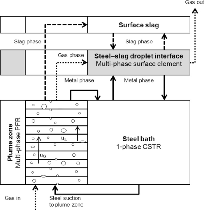
A new approach was adopted for considering the vertical distribution of composition, temperature, pressure and element activities in the plume zone. The process model represents the AOD converter as a combination of a Plug Flow Reactor (PFR), a Continuously Stirred Tank Reactor (CSTR) and a top slag zone. All the chemical reactions are assumed to take place in the plume zone simulated by the PFR, which is divided vertically into numerous computational cells. After the PFR, the slag phase ends up in a separate surface slag zone and the metal phase continues to the CSTR and eventually circulates back to the lowest computational cell of the PFR. This is a significant improvement over traditional approaches, which use average values for the whole reaction zone. However, the oxides in the surface slag were considered non-reducible and hence reactions between the metal bath and top slag were not taken into account.

As discussed above, the mathematical models for the side- and top-blown decarburisation stage have evolved from simplistic descriptions into complex process models capable of accurate predictions. However, much less attention has been paid to the reduction stage. Although numerous studies have been conducted on the emulsification of slag^{31,32,33,34,35,36,37,38,39,40,41,42)} and reduction of slag^{18,43,44,45,46)} as separate research fields, a phenomena-based model capable of combining the present knowledge of both phenomena has not been previously discussed in the literature.

3. Derivation of a Mathematical Model for the Reduction Stage

In the previous work,^6,7) the surface slag was considered non-reducible and hence had no active role during decarburisation. Therefore, it is obvious that the initial model cannot be used to observe the reduction stage. In this paper, a new reaction model is proposed for considering the reduction stage at the end of the AOD treatment.

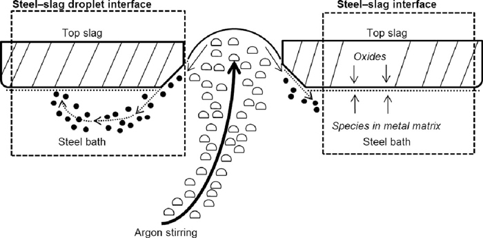
During the reduction stage, two reaction interfaces can be identified: the steel–slag droplet interface and the steel–slag interface (see Fig. 1). In this context, emulsification of slag droplets is caused by the turning around of fluid flow at the top of the plume eye.⁴⁷⁾ When the critical interfacial velocity is exceeded, the surface area of the slag droplets is typically multifold compared to the plain interfacial area of the steel-slag interface.³³⁾ Moreover, the contribution of the steel–slag droplet interface is accentuated by the high mass transfer rate resulting from vigorous argon stirring and small slag droplet size. The steel–slag interface is handicapped by the slow mass transfer of slag species caused by inefficient mixing in the top slag.

In the model derived in this paper, it is assumed that the contribution of the steel–slag interface to the total reaction rates is negligible and that the dominating phenomena during the reduction stage can be accurately described by reactions occurring on the surface of the emulsified slag droplets. Furthermore, it is assumed that the species from the top slag, metal bulk and plume gas phase establish a thermodynamic equilibrium at the surface of the slag droplets, in which only one average composition, one average temperature and one average surface area are considered. From a modelling perspective, the steel–slag droplet interface is represented by a multi-phase surface element with zero thickness. The model derived in this paper is programmed with C/C++ and coupled with the previously proposed model for side-blowing decarburisation stages as illustrated in Fig. 2.

Fig. 1.

Schematic illustration of the two interfaces considered in the model.

Fig. 2.

Schematic illustration of the modified process model.

3.1. Reaction System

The total number of species considered in the system is 21. The metal phase is a concentrated Fe–Cr–Mn–Si–C–O–N–Ni alloy, while the gas phase is considered to consist of O₂, CO, CO₂, N₂ and Ar.

The liquid top slag is constituted by FeO, Cr₂O₃, MnO, SiO₂, CaO, MgO, Al₂O₃ and MeOx, which is used to describe oxides that are excluded from the model. For all purposes, CaF₂ was taken here as the calcium ion. Chromium oxide is assumed to exist only in its trivalent form, due to the high basicity of decarburisation slags.⁴⁸⁾ At first, it is assumed that direct accumulation of CaO into the slag takes place, to act as a slag former.

The approach proposed by Järvinen^5,6) is employed here for solving the multi-phase system considered in the surface element. In this approach, it is assumed that if the chemical rate is sufficiently high, the reaction rates will be controlled by mass transfer only, and the exact value of the forward reaction constant k_f becomes irrelevant as long as it satisfies the equilibrium condition. This enables the simultaneous solution of thermodynamic equilibrium at the interface and the mass transfer of species onto the interface. This approach has been tested successfully for modelling the plume zone of the AOD vessel during the decarburisation stage^5,6,7) and for chemical heating in the CAS-OB process.⁴⁹⁾ The proof of this approach is not repeated here.

Taking these considerations into account, the chemical reactions and their corresponding rate expressions can be formulated as follows:   

$$\begin{array}{c}{\text{O}}_2\left(\text{g}\right)\rightleftharpoons 2\underset{\_}{\text{O}}\\ {\text{R}}_0^{\prime \prime }={\text{k}}_{\text{f},\mathrm{\hspace{0.17em} }\text{R}0}\left({\text{p}}_{{\text{O}}_2}-\frac{{\text{a}}_{\text{O}}^2}{{\text{K}}_{\text{eq},\mathrm{\hspace{0.17em} }0}}\right)\end{array}$$(1)

  

$$\begin{array}{c}\underset{\_}{\mathrm{C}}+\frac{1}{2}{\text{O}}_2\left(\text{g}\right)\rightleftharpoons \text{CO}\left(\text{g}\right)\\ {\text{R}}_1^{\prime \prime }={\text{k}}_{\text{f},\mathrm{\hspace{0.17em} }\text{R}1}\left({\text{a}}_{\underset{\_}{\mathrm{C}}}{\text{p}}_{{\text{O}}_2}^{0.5}-\frac{{\text{p}}_{\text{CO}}}{{\text{K}}_{\text{eq},\mathrm{\hspace{0.17em} }1}}\right)\end{array}$$(2)

  

$$\begin{array}{c}\underset{\_}{\mathrm{C}}+{\text{O}}_2(\text{g})\rightleftharpoons {\text{CO}}_2(\text{g})\\ {\text{R}}_2^{\prime \prime }={\text{k}}_{\text{f},\mathrm{\hspace{0.17em} }\text{R}2}\left({\text{a}}_{\underset{\_}{\mathrm{C}}}{\text{p}}_{{\text{O}}_2}-\frac{{\text{p}}_{{\text{CO}}_2}}{{\text{K}}_{\text{eq},\mathrm{\hspace{0.17em} }2}}\right)\end{array}$$(3)

  

$$\begin{array}{c}\underset{\_}{\mathrm{F}\mathrm{e}}+\frac{1}{2}{\text{O}}_2(\text{g})\rightleftharpoons \left(\text{FeO}\right)\\ {\text{R}}_3^{\prime \prime }={\text{k}}_{\text{f},\mathrm{\hspace{0.17em} }\text{R}3}\left({\text{a}}_{\underset{\_}{\mathrm{F}\mathrm{e}}}{\text{p}}_{{\text{O}}_2}^{0.5}-\frac{{\text{a}}_{\left(\text{FeO}\right)}}{{\text{K}}_{\text{eq},\mathrm{\hspace{0.17em} }3}}\right)\end{array}$$(4)

  

$$\begin{array}{c}2 \underset{\_}{\mathrm{C}\mathrm{r}}+\frac{3}{2}{\text{O}}_2\left(\text{g}\right)\rightleftharpoons \left({\text{Cr}}_2{\text{O}}_3\right)\\ {\text{R}}_4^{\prime \prime }={\text{k}}_{\text{f},\mathrm{\hspace{0.17em} }\text{R}4}\left({\text{a}}_{\underset{\_}{\mathrm{C}\mathrm{r}}}^2{\text{p}}_{{\text{O}}_2}^{1.5}-\frac{{\text{a}}_{({\text{Cr}}_2{\text{O}}_3)}}{{\text{K}}_{\text{eq},\mathrm{\hspace{0.17em} }4}}\right)\end{array}$$(5)

  

$$\begin{array}{c}\underset{\_}{\text{Mn}}+\frac{1}{2}{\text{O}}_2\left(\text{g}\right)\rightleftharpoons \left(\text{MnO}\right)\\ {\text{R}}_5^{\prime \prime }={\text{k}}_{\text{f},\mathrm{\hspace{0.17em} }\text{R}5}\left({\text{a}}_{\underset{\_}{\text{Mn}}}{\text{p}}_{{\text{O}}_2}^{0.5}-\frac{{\text{a}}_{\left(\text{MnO}\right)}}{{\text{K}}_{\text{eq},\mathrm{\hspace{0.17em} }5}}\right)\end{array}$$(6)

  

$$\begin{array}{c}\underset{\_}{\text{Si}}+{\text{O}}_2(\text{g})\rightleftharpoons \left({\text{SiO}}_2\right)\\ {\text{R}}_6^{\prime \prime }={\text{k}}_{\text{f},\mathrm{\hspace{0.17em} }\text{R}6}\left({\text{a}}_{\underset{\_}{\text{Si}}}{\text{p}}_{{\text{O}}_2}-\frac{{\text{a}}_{({\text{SiO}}_2)}}{{\text{K}}_{\text{eq},\mathrm{\hspace{0.17em} }6}}\right)\end{array}$$(7)

The reactions are fully reversible in order to enable both oxidation of dissolved elements in the steel bath and reduction of species in the top slag. This approach leads to a complex system of steel-slag reactions, in which elements with the highest oxygen affinities will reduce oxides of elements with a lower oxygen affinity. The reactions given in Eqs. (2), (3), (4), (5), (6), (7) are formulated with gaseous oxygen, but because there is practically no gaseous oxygen available during the reduction stage, the reactions effectively consume the dissolved oxygen through Eq. (1). However, the mass transfer of gas species is far more efficient than that of the liquid species, and it follows that the mass transfer of gaseous oxygen does not limit the reaction rates similar to the mass transfer of dissolved oxygen.

Although reactions with refractory materials are excluded from this work, the effect of refractory wear on the slag composition has been taken into account with a fixed constant for dissolution rate of refractory material into the slag. Moreover, the effect of refractory wear on the converter geometry has been taken into account as a loss of refractory lining thickness per heat. The converter geometry affects, for example, the height of the steel bath and the thickness of the top slag layer. Reactions between the top slag and the refractory lining are taken into account with an average dissolution rate of refractory material into the top slag, which is calculated from the loss of refractory lining thickness per heat.

It should be noted here that the conservation of mass and heat are solved consequently, not simultaneously. However, if sufficiently small time steps are used, no significant inaccuracy is caused, while the stability of calculations is substantially improved.

3.2. Conservation of Mass

Discretisation of the conservation equations is carried out with an implicit finite-difference method, using a 1^st order Euler-method for time integration. Conservation of species i in the metal (8), gas (9) and slag phase (10) at the interface are expressed below:   

$${\mathrm{\Gamma }}_{\text{L},\mathrm{\hspace{0.17em} }\text{i}}{\text{h}}_{\text{L}}^{\text{SE}}{\rho }_{\text{L}}\left({\text{y}}_{\text{i}}^{\text{Bath}}-{\text{y}}_{\text{i}}^{\text{SE}}\right)-{\displaystyle \sum }_{\text{k}=1}^{{\text{N}}_{\text{R}}}{\mathrm{\Gamma }}_{\text{L},\mathrm{\hspace{0.17em} }\text{i}}{\overline{\nu }}_{\text{i},\mathrm{\hspace{0.17em} }\text{k}}{\text{R}}_{\text{k}}^{\prime \prime }=0$$(8)

  

$${\mathrm{\Gamma }}_{\text{G},\mathrm{\hspace{0.17em} }\text{i}}{\text{h}}_{\text{G}}^{\text{SE}}{\rho }_{\text{G}}\left({\text{y}}_{\text{i}}^{\text{Plume}}-{\text{y}}_{\text{i}}^{\text{SE}}\right)-{\displaystyle \sum }_{\text{k}=1}^{{\text{N}}_{\text{R}}}{\mathrm{\Gamma }}_{\text{G},\mathrm{\hspace{0.17em} }\text{i}}{\overline{\nu }}_{\text{i},\mathrm{\hspace{0.17em} }\text{k}}{\text{R}}_{\text{k}}^{\prime \prime }=0$$(9)

  

$${\mathrm{\Gamma }}_{\text{S},\mathrm{\hspace{0.17em} }\text{i}}{\text{h}}_{\text{S}}^{\text{SE}}{\rho }_{\text{S}}\left({\text{y}}_{\text{i}}^{\text{Slag}}-{\text{y}}_{\text{i}}^{\text{SE}}\right)-{\displaystyle \sum }_{\text{k}=1}^{{\text{N}}_{\text{R}}}{\mathrm{\Gamma }}_{\text{S},\mathrm{\hspace{0.17em} }\text{i}}{\overline{\nu }}_{\text{i},\mathrm{\hspace{0.17em} }\text{k}}{\text{R}}_{\text{k}}^{\prime \prime }=0$$(10)

where SE, Bath, Plume and Slag denote the surface element, steel bath, plume gas and the top slag, respectively. Γ are binary variables predefined 1 for species present in phase and 0 for others. ${\overline{\nu }}_{\text{i}, \text{k}, \text{f}}$ is defined here as the mass-based stoichiometric coefficient of species i in a reaction k:   

$${\overline{\nu }}_{\text{i},\mathrm{\hspace{0.17em} }\text{k}}={\nu }_{\text{i},\mathrm{\hspace{0.17em} }\text{k}}\frac{{\text{M}}_{\text{i}}}{{\text{M}}_{\text{K},\mathrm{\hspace{0.17em} }\text{k},\mathrm{\hspace{0.17em} }\text{f}}}$$(11)

where M_K.k is the molar mass of a key component in reaction k, that is, a component that is used to define the reaction rate. For the reactions given in Eqs. (1), (2), (3), (4), (5), (6), (7), the key components are O₂, C, C, Fe, Cr, Mn and Si respectively. The compositions and temperatures of the bulk phases must also be updated. The conservation of species i in the metal bath (12), highest plume cell (13) and top slag (14) are expressed by:   

$$-{\text{h}}_{\text{L}}^{\text{SE}}{\rho }_{\text{L}}{\text{A}}_{\text{SE}}\left({\text{y}}_{\text{i}}^{\text{Bath}}-{\text{y}}_{\text{i}}^{\text{SE}}\right)=\frac{{\text{m}}_{\text{Bath}}^{\text{t}}{\text{y}}_{\text{Bath}}^{\text{t}}-{\text{m}}_{\text{Bath}}^{\text{t}-1}{\text{y}}_{\text{Bath}}^{\text{t}-1}}{\mathrm{\Delta }\text{t}}$$(12)

  

$$-{\text{h}}_{\text{G}}^{\text{SE}}{\rho }_{\text{G}}{\text{A}}_{\text{SE}}\left({\text{y}}_{\text{i}}^{\text{Plume}}-{\text{y}}_{\text{i}}^{\text{SE}}\right)=\frac{{\text{m}}_{\text{Plume}}^{\text{t}}{\text{y}}_{\text{Plume}}^{\text{t}}-{\text{m}}_{\text{Plume}}^{\text{t}-1}{\text{y}}_{\text{Plume}}^{\text{t}-1}}{\mathrm{\Delta }\text{t}}$$(13)

  

$$-{\text{h}}_{\text{S}}^{\text{SE}}{\rho }_{\text{S}}{\text{A}}_{\text{SE}}\left({\text{y}}_{\text{i}}^{\text{Slag}}-{\text{y}}_{\text{i}}^{\text{SE}}\right)=\frac{{\text{m}}_{\text{Slag}}^{\text{t}}{\text{y}}_{\text{Slag}}^{\text{t}}-{\text{m}}_{\text{Slag}}^{\text{t}-1}{\text{y}}_{\text{Slag}}^{\text{t}-1}}{\mathrm{\Delta }\text{t}}$$(14)

where Δt is the time step. Conservation of total mass of metal bath, plume gas and top slag is expressed according to Eqs. (15), (16), (17), respectively.   

$$-{\displaystyle \sum }_{\text{i}=1}^{\text{N}}{\mathrm{\Gamma }}_{\text{L},\mathrm{\hspace{0.17em} }\text{i}}{\text{h}}_{\text{L}}^{\text{SE}}{\rho }_{\text{L}}{\text{A}}_{\text{SE}}\left({\text{y}}_{\text{i}}^{\text{Bath}}-{\text{y}}_{\text{i}}^{\text{SE}}\right)=\frac{{\text{m}}_{\text{Bath}}^{\text{t}}-{\text{m}}_{\text{Bath}}^{\text{t}-1}}{\mathrm{\Delta }\text{t}}$$(15)

  

$$-{\displaystyle \sum }_{\text{i}=1}^{\text{N}}{\mathrm{\Gamma }}_{\text{G},\mathrm{\hspace{0.17em} }\text{i}}{\text{h}}_{\text{G}}^{\text{SE}}{\rho }_{\text{G}}{\text{A}}_{\text{SE}}\left({\text{y}}_{\text{i}}^{\text{Plume}}-{\text{y}}_{\text{i}}^{\text{SE}}\right)=\frac{{\text{m}}_{\text{Plume}}^{\text{t}}-{\text{m}}_{\text{Plume}}^{\text{t}-1}}{\mathrm{\Delta }\text{t}}$$(16)

  

$$-{\displaystyle \sum }_{\text{i}=1}^{\text{N}}{\mathrm{\Gamma }}_{\text{S},\mathrm{\hspace{0.17em} }\text{i}}{\text{h}}_{\text{S}}^{\text{SE}}{\rho }_{\text{S}}{\text{A}}_{\text{SE}}\left({\text{y}}_{\text{i}}^{\text{Slag}}-{\text{y}}_{\text{i}}^{\text{SE}}\right)=\frac{{\text{m}}_{\text{Slag}}^{\text{t}}-{\text{m}}_{\text{Slag}}^{\text{t}-1}}{\mathrm{\Delta }\text{t}}$$(17)

In order to be physically exact, it would also be necessary to consider conservation of mass in the slag droplets. More specifically, conservation of mass should be solved for a distribution of slag droplet sizes. In practice, considering the transient slag droplet distribution, the resulting distribution of mass transfer properties and residence times, and the effect of the reactions on the slag droplets require a computationally slow CFD-based approach. This would be contradictory to the objective of developing a process model for the reduction stage. Consequently, the conservation of mass in the slag droplets as a boundary condition was excluded from the model.

3.3. Conservation of Heat

The conservation of heat in the isothermal surface element is defined by heat transfer and reaction enthalpies (18).   

$$\begin{array}{l}{\alpha }_{\text{L}}^{\text{SE}}\left({\text{T}}_{\text{Bath}}-{\text{T}}_{\text{SE}}\right)+{\alpha }_{\text{G}}^{\text{SE}}\left({\text{T}}_{\text{Gas}}-{\text{T}}_{\text{SE}}\right)+{\alpha }_{\text{S}}^{\text{SE}}\left({\text{T}}_{\text{Slag}}-{\text{T}}_{\text{SE}}\right)\\ +{\displaystyle \sum }_{\text{k}=1}^{{\text{N}}_{\text{R}}}{\text{R}}_{\text{k}}^{\prime \prime }\mathrm{\Delta }{\text{h}}_{\text{k}}=0\end{array}$$(18)

Conservation of heat in the steel bath (19), plume gas (20) and the top slag (21) can be formulated mathematically as:   

$$\begin{array}{l}-{\alpha }_{\text{L}}^{\text{SE}}{\text{A}}_{\text{SE}}\left({\text{T}}_{\text{Bath}}-{\text{T}}_{\text{SE}}\right)-{\displaystyle \sum }_{\text{i}=1}^{\text{N}}{\displaystyle \sum }_{\text{k}=1}^{{\text{N}}_{\text{R}}}{\mathrm{\Gamma }}_{\text{L},\mathrm{\hspace{0.17em} }\text{i}}{\overline{\nu }}_{\text{i}, \text{k}}{\text{R}}_{\text{k}}^{\prime \prime }{\text{A}}_{\text{SE}}{\text{c}}_{\text{p},\mathrm{\hspace{0.17em} }\text{i}} –{\mathrm{\Phi }}_{\text{Lining}}\\ =\frac{{\text{m}}_{\text{Bath}}{\text{c}}_{\text{p},\mathrm{\hspace{0.17em} }\text{Bath}}\left({\text{T}}_{\text{Bath}}^{\text{t}}-{\text{T}}_{\text{Bath}}^{\text{t}-1}\right)}{\mathrm{\Delta }\text{t}}\end{array}$$(19)

  

$$\begin{array}{l}-{\alpha }_{\text{G}}^{\text{SE}}{\text{A}}_{\text{SE}}\left({\text{T}}_{\text{Plume}}-{\text{T}}_{\text{SE}}\right)-{\displaystyle \sum }_{\text{i}=1}^{\text{N}}{\displaystyle \sum }_{\text{k}=1}^{{\text{N}}_{\text{R}}}{\mathrm{\Gamma }}_{\text{G}, \text{i}}{\overline{\nu }}_{\text{i},\mathrm{\hspace{0.17em} }\text{k}}{\text{R}}_{\text{k}}^{\prime \prime }{\text{A}}_{\text{SE}}{\text{c}}_{\text{p},\mathrm{\hspace{0.17em} }\text{i}} \\ =\frac{{\text{m}}_{\text{Plume}}{\text{y}}_{\text{Gas}}{\text{c}}_{\text{p},\mathrm{\hspace{0.17em} }\text{Plume}}\left({\text{T}}_{\text{Plume}}^{\text{t}}-{\text{T}}_{\text{Plume}}^{\text{t}-1}\right)}{\mathrm{\Delta }\text{t}}\end{array}$$(20)

  

$$\begin{array}{l}-{\alpha }_{\text{S}}^{\text{SE}}{\text{A}}_{\text{SE}}\left({\text{T}}_{\text{Slag}}-{\text{T}}_{\text{SE}}\right)-{\displaystyle \sum }_{\text{i}=1}^{\text{N}}{\displaystyle \sum }_{\text{k}=1}^{{\text{N}}_{\text{R}}}{\mathrm{\Gamma }}_{\text{S},\mathrm{\hspace{0.17em} }\text{i}}{\overline{\nu }}_{\text{i},\mathrm{\hspace{0.17em} }\text{k}}{\text{R}}_{\text{k}}^{\prime \prime }{\text{A}}_{\text{SE}}{\text{c}}_{\text{p},\mathrm{\hspace{0.17em} }\text{i}}–{\mathrm{\Phi }}_{\text{Slag}}\\ =\frac{{\text{m}}_{\text{Slag}}{\text{c}}_{\text{p},\mathrm{\hspace{0.17em} }\text{Slag}}\left({\text{T}}_{\text{Slag}}^{\text{t}}-{\text{T}}_{\text{Slag}}^{\text{t}-1}\right)}{\mathrm{\Delta }\text{t}}\end{array}$$(21)

where y_Gas is the fraction of gas in the plume cell. Φ_Lining and Φ_Slag are the heat losses through lining (22) and through top slag (23), respectively, and are defined as:   

$${\mathrm{\Phi }}_{\text{Lining}}={\text{q}}_{\text{Lining}}{\text{A}}_{\text{Lining}}$$(22)

  

$${\mathrm{\Phi }}_{\text{Slag}}={\text{q}}_{\text{Slag}}{\text{A}}_{\text{Slag}}$$(23)

where heat loss fluxes through lining and slag surface are q_Lining = 12500 W/m² and q_Slag = 8000 W/m², respectively.⁵⁰⁾ A more sophisticated approach for treating the heat losses can be derived in further work.

3.4. Rate of Slag Droplet Formation

As mentioned earlier, the surface area of the emulsified droplets is taken as the total reaction area in the model. By assuming a uniform droplet size, the total surface area of the droplets can be approximated using Eq. (24).   

$${\text{A}}_{\text{D}}={\int }_{\text{t}-{\text{t}}_{\text{res}}}^{\text{t}}\pi {\text{d}}_{\text{D}}^2\left(\text{t}\right){\dot{\text{N}}}_{\text{D}}(\text{t})\text{dt}\approx {\displaystyle \sum }_{\text{t}-{\text{t}}_{\text{res}}}^{\text{t}}\pi {\text{d}}_{\text{D}}^2\left(\text{t}\right){\dot{\text{N}}}_{\text{D}}(\text{t})\mathrm{\Delta }t$$(24)

where t_res is the residence time of the slag droplets in the steel bath. The average residence time can be defined as the ratio of emulsified slag volume to droplet volume generated per time unit:³⁴⁾   

$${\text{t}}_{\text{res}}=\frac{{\text{V}}_{\text{em}}}{{\dot{\text{V}}}_{\text{D}}}$$(25)

The droplet size used in the calculations is given by the equation suggested by Wei & Oeters:³⁶⁾   

$${\text{d}}_{\text{D}}=\frac{3}{8}\frac{{\rho }_{\text{S}}{\text{u}}_{\text{i}}^2}{\text{g}\left({\rho }_{\text{L}}-{\rho }_{\text{S}}\right)}\left\{1-{\left[1-\frac{128\sigma \text{g}\left({\rho }_{\text{L}}-{\rho }_{\text{S}}\right)cos\alpha }{3{\rho }_{\text{S}}^2{\text{u}}_{\text{i}}^4}\right]}^{\frac{1}{2}}\right\}$$(26)

Here, the droplet size calculated with Eq. (26) is taken as the Sauter mean diameter of the droplets formed at a given time step. The average diameter of the droplets residing in the bath is calculated from Eq. (27):   

$${\text{d}}_{\text{D}}^{\text{AVG}}(\text{t})=\frac{1}{{\text{t}}_{\text{res}}}{\displaystyle \sum }_{\text{t}-{\text{t}}_{\text{res}}}^{\text{t}}{\text{d}}_{\text{D}}(\text{t})\mathrm{\Delta }\text{t}$$(27)

The use of the residence time as a fitting parameter will be discussed later in Part II. Based on energy flow balance, Oeters^36,47) has derived an equation for calculating the number of droplets formed per time unit:   

$${\dot{\text{N}}}_{\text{D}}=\frac{0.4153\text{D}{\rho }_{\text{S}}^{\frac{1}{2}}{\eta }_{\text{S}}^{\frac{1}{2}}{\text{L}}^{\frac{1}{2}}{\text{u}}_{\text{i}}^{\frac{5}{2}}}{{\text{d}}_{\text{D}}^2\sigma +\frac{1}{6}\pi {\text{d}}_{\text{D}}^4\text{g}\left({\rho }_{\text{L}}-{\rho }_{\text{S}}\right)cos\alpha }$$(28)

where D is the diameter of the plume zone at the interface, L is the thickness of the interfacial layer, u_i is velocity, η is the viscosity of the slag, σ is the interfacial surface tension, ρ_m is the density of the metal phase, ρ_s is the density of the slag phase and α is the angle between inertial and vertical force. From this equation, it is apparent that the number of droplets formed increases with a thickening slag layer and increasing interfacial velocity, respectively.⁴⁷⁾ The values used for this equation are discussed in the following paragraphs.

Based on results with CFD modelling,⁵¹⁾ the plume diameter was set to 1.5 m. The interfacial velocity u_i is defined by:⁴⁷⁾   

$${\text{u}}_{\text{i}}={\text{u}}_{\text{L}}\cdot \text{K}$$(29)

where u_L is given by Eq. (30) and K is obtained iteratively from Eq. (31).   

$${\text{u}}_{\text{L}}={\text{u}}_{\text{L},\mathrm{\hspace{0.17em} }0}+\frac{2}{3}{\left[2\text{g}\left(1-\frac{{\rho }_{\text{S}}}{{\rho }_{\text{L}}}\right)\text{L}cos\alpha \right]}^{\frac{1}{2}}$$(30)

  

$$\begin{array}{c}\text{K}=0.1367{\left(\frac{{\rho }_{\text{L}}}{{\rho }_{\text{S}}}\right)}^{\frac{2}{3}}{\left(\frac{{\text{u}}_{\text{L}}\text{L}}{{\nu }_{\text{S}}}\right)}^{\frac{1}{3}}{\left(\frac{{\text{u}}_{\text{L}}\text{L}}{{\nu }_{\text{L}}}\right)}^{-\frac{2}{15}}\\ {\left[\left(1-\text{K}\right)\left(0.1108-0.0693\text{K}\right)\right]}^{\frac{2}{15}}\end{array}$$(31)

From Eqs. (29), (30) and (31) it follows that the interfacial velocity is effectively independent from the gas flow rate. The entering velocity of the steel stream is defined by the height of the top of plume above surface slag:   

$${\text{u}}_{\text{L},\mathrm{\hspace{0.17em} }0}=\sqrt{2\text{gh}}$$(32)

It has been shown that the spout height fluctuates strongly during blowing.⁵²⁾ Some mathematical expressions for the height of the spout have been suggested for Vacuum Oxygen Decarburisation⁵³⁾ and ladle treatments.⁵⁴⁾ However, these results cannot be extrapolated to the AOD process, as it employs strongly eccentric side-blowing and substantially higher flow velocities. Therefore, it was assumed that the spout reaches the slag surface, but does not rise above it.

The angle between inertial and vertical force was set to α = 30° based on laboratory scale experiments.⁴²⁾ A linear approximation has been used for calculating the density of the steel bath with respect to temperature:   

$${\rho }_{\text{L}}=8586-0.8567\cdot \text{T}$$(33)

The density of the slag phase is approximated with partial molar volumes:⁵⁵⁾   

$${\rho }_{\text{S}}={\displaystyle \sum }_{\text{i}=1}^{\text{N}}\frac{{\text{M}}_{\text{i}}{\text{x}}_{\text{i}}}{{\overline{\text{V}}}_{\text{i}}}$$(34)

The interfacial surface tension of the top slag was set to σ = 0.49 N/m.⁵⁶⁾ The slag viscosity model proposed by Forsbacka et al.⁵⁷⁾ is used for calculating the viscosity of the top slag. This model is basically an extension of the modified Urbain model⁵⁸⁾ for the Al₂O₃–CaO–CrO–Cr₂O₃–’FeO’–MgO–SiO₂ system. The dynamic viscosity of the slag is defined by a Weymann-Frenkel relation:   

$$\eta ={\text{ATe}}^{\frac{1\mathrm{\hspace{0.17em} }000\text{B}}{\text{T}}}$$(35)

Fig. 3.

Schematic illustration of the slag droplet model.

where model parameter A defined by the compensation law:   

$$-ln\text{A}=\text{mB}+\text{n}$$(36)

where n is constant and m is calculated based on slag composition and adjustable model coefficients.

3.5. Mass and Heat Transfer Coefficients

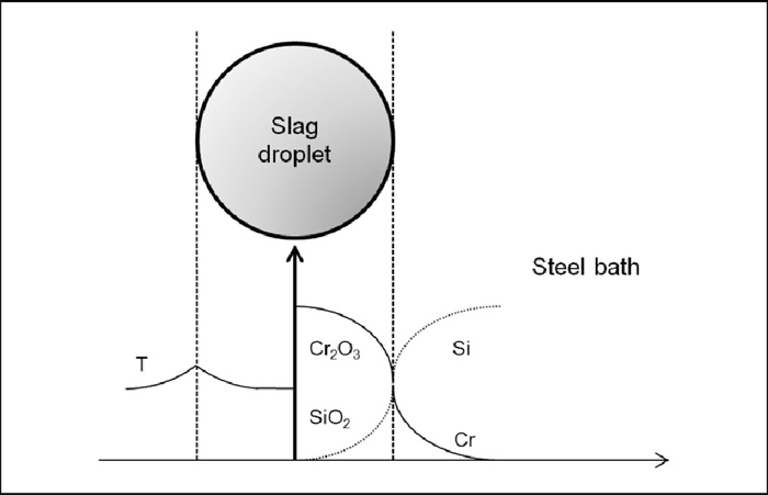
The surface renewal model proposed by Higbie⁵⁹⁾ has been used for determining heat and mass transfer constants in the boundary layers on both sides of the slag droplet as illustrated in Fig. 3. The mass and heat transfer coefficients for metal, gas and slag phase are given by:   

$${\text{h}}_{\text{L}}^{\text{D}}=1.28\sqrt{\frac{{\text{D}}_{\text{m},\mathrm{\hspace{0.17em} }\text{L}}\cdot {\text{u}}_{\text{S},\mathrm{\hspace{0.17em} }\text{D}}}{{\text{d}}_{\text{D}}^{\text{AVG}}}};\mathrm{\hspace{0.17em} }{\alpha }_{\text{L}}^{\text{D}}=1.28{\rho }_{\text{L}}{\text{c}}_{\text{p},\mathrm{\hspace{0.17em} }\text{L}}\sqrt{\frac{{\lambda }_{\text{L}}\cdot {\text{u}}_{\text{S},\mathrm{\hspace{0.17em} }\text{D}}}{{\rho }_{\text{L}}{\text{c}}_{\text{p},\mathrm{\hspace{0.17em} }\text{L}}{\text{d}}_{\text{D}}^{\text{AVG}}}}$$(37)

  

$${\text{h}}_{\text{G}}^{\text{D}}=1.28\sqrt{\frac{{\text{D}}_{\text{m},\mathrm{\hspace{0.17em} }\text{G}}\cdot {\text{u}}_{\text{S},\mathrm{\hspace{0.17em} }\text{b}}}{{\text{d}}_{\text{b}}}};\mathrm{\hspace{0.17em} }{\alpha }_{\text{G}}^{\text{D}}=1.28{\rho }_{\text{G}}{\text{c}}_{\text{p},\mathrm{\hspace{0.17em} }\text{G}}\sqrt{\frac{{\lambda }_{\text{G}}\cdot {\text{u}}_{\text{S},\mathrm{\hspace{0.17em} }\text{b}}}{{\rho }_{\text{G}}{\text{c}}_{\text{p},\mathrm{\hspace{0.17em} }\text{G}}{\text{d}}_{\text{b}}}}$$(38)

  

$${\text{h}}_{\text{S}}^{\text{D}}=12\frac{{\text{D}}_{\text{m},\mathrm{\hspace{0.17em} }\text{S}}}{{\text{d}}_{\text{D}}^{\text{AVG}}};\mathrm{\hspace{0.17em} }{\alpha }_{\text{S}}^{\text{D}}=12\frac{{\lambda }_{\text{S}}}{{\text{d}}_{\text{D}}^{\text{AVG}}}$$(39)

where D_m is the molecular diffusivity of species i, ${\text{d}}_{\text{D}}^{\text{AVG}}$ is the average diameter of emulsified slag droplets, d_b is the average diameter of a gas bubble, λ is the heat conductivity, and c_p is the specific thermal capacity.

Some diffusion coefficients in liquid steel are illustrated in Table 2. However, as the model employs an effective diffusion model, only one effective diffusion coefficient is determined for each phase. The molecular diffusion coefficients for the steel and slag phases are set to D_{m, L} = D_{m, S} = 4.0×10^–9 m/s², which are roughly in the same range as the values provided in Table 2. The temperature-dependency of diffusion coefficients is excluded in this work. For the gas phase, the following equation is used:   

$${\text{D}}_{\text{m},\mathrm{\hspace{0.17em} }\text{G}}=0.21\cdot {10}^{-4}\cdot \frac{{\left(\frac{\text{T}}{298}\right)}^{1.5}}{\frac{\text{p}}{{\text{p}}_{\text{N}}}}$$(40)

The initial proposition is that the slip velocity between the steel bath and the slag droplet equals the terminal rising velocity of the slag droplet in the y-direction. At the terminal rising velocity in y-direction, the following force balance must hold:   

$${\text{F}}_{\text{B}}={\text{F}}_{\text{D}}+{\text{F}}_{\text{G}}$$(41)

where F_B, F_D and F_G are the buoyancy force, drag force and graviation acting on the droplet, respectively. The terminal velocity in the y-direction is then given by:   

$${\text{v}}_{\text{t}}=\sqrt{\frac{4{\text{gd}}_{\text{D}}^{\text{AVG}}}{3{\text{C}}_{\text{d}}}\frac{({\rho }_{\text{L}}-{\rho }_{\text{S}})}{{\rho }_{\text{L}}}}$$(42)

Table 2. Diffusion coefficients in liquid iron at 1873 K.⁶⁰⁾

Species	Dm x 10–9 [m2/s]
Cr	3–5
Mn	3.5–20
Si	2.5–12
C	4–20
O	2.5–20
N	6–20
Ni	4.5–5.6

In the low Reynolds range (Re < 1000) the C_d can be solved as presented below.⁶¹⁾   

$${\text{C}}_{\text{d}}=\frac{24}{\text{Re}}\left(1+0.125{\text{Re}}^{0.72}\right)$$(43)

where the Reynolds number is given by:   

$$\text{Re}=\frac{{\rho }_{\text{L}}{\text{v}}_{\text{t}}{\text{d}}_{\text{D}}^{\text{AVG}}}{{\mu }_{\text{L}}}$$(44)

The characteristic relaxation time, representing the time to reach 63% of the equilibrium velocity is given by:⁶²⁾   

$${\tau }_{\text{r}}=\frac{{\text{m}}_{\text{D}}{\text{C}}_{\text{D}}}{3\pi {\mu }_{\text{L}}{\text{d}}_{\text{D}}^{\text{AVG}}}$$(45)

For this example, the following properties are assumed: ρ_L = 7000 kg/m³, ρ_S = 2650 kg/m³, μ_S = 0.0049 kg/(m·s) and d_D = 0.001 m. The resulting numerical solution yields C_d ≈ 0.945, v_t ≈ 0.0928 m/s and τ_r ≈ 0.0284 s for the drag coefficient, terminal rising velocity and relaxation time, respectively. This suggests that the average rising velocity is very close to the terminal rising velocity and therefore it should not cause a significant error to assume that the average rising velocity equals the terminal rising velocity.

It has been shown that both bubble size and gas-metal slip velocity vary strongly within the AOD vessel.^63,64) Iguchi et al.⁶³⁾ have reported a bubble size of 25 mm and a corresponding slip velocity of 0.5–0.7 m/s in the Fe–Ar system in the plume zone of the vessel. Tilliander et al.⁶⁴⁾ have reported slip velocities in the order of 0.01 m/s outside the plume area during oxygen-blowing. Moreover, bubble size increased slightly towards the surface of the plume eye, being approximately 45 mm in the vicinity of the surface. In this paper, bubble size and corresponding velocity difference with the liquid phase were estimated by the following equations:^65,66)   

$${\text{d}}_{\text{b}}=0.168\sqrt{\frac{\sigma }{{\rho }_{\text{L}}^{\frac{2}{3}}}}$$(46)

  

$${\text{u}}_{\text{S},\mathrm{\hspace{0.17em} }\text{b}}={\left(\frac{2\sigma }{{\rho }_{\text{L}}{\text{d}}_{\text{b}}}+\frac{{\text{gd}}_{\text{b}}}{2}\right)}^{\frac{1}{2}}$$(47)

Given σ = 1 N/m and ρ_L = 7000 kg/m³, these equations yield d_b ≈ 8.8 mm and u_S,b ≈ 0.27 m/s. Gas hold-up, representing here the volume fraction of the gas phase in the plume zone, was set to 0.2 as reported in earlier work.⁷⁾

3.6. Thermodynamic Behaviour of Species

Equilibrium constants are calculated using the enthalpy and entropy data presented in Table 3. The average reaction enthalpies and entropies at 1800–2100 K were first calculated for pure species using the thermodynamic database of the HSC Chemistry⁶⁷⁾ and then converted to the selected standard states using literature data.⁶⁸⁾ The Henrian reference state (1 mol-%) is employed for the liquid species, while the reference states of the gaseous and slag species are pure gaseous species and pure liquid species, respectively. The equilibrium constant of reaction k is defined by:

Table 3. Average reaction enthalpies and entropies at 1800–2100 K.^67,68)

Reaction	ΔH [J/mol]	Δh [J/kg]	ΔS [J/(mol·K)]
${\text{O}}_2\left(\text{g}\right)\rightleftharpoons 2\underset{\_}{\text{O}}$	–234304.0	–7322274.6	–50.0
$\underset{\_}{\text{C}}+\frac{1}{2}{\text{O}}_2\left(\text{g}\right)\rightleftharpoons \text{CO}\left(\text{g}\right)$	–141141.4	–11751011.4	67.0
$\underset{\_}{\text{C}}+{\text{O}}_2(\text{g})\rightleftharpoons {\text{CO}}_2(\text{g})$	–419249.5	–34905457.7	–16.9
$\underset{\_}{\text{Fe}}+\frac{1}{2}{\text{O}}_2\left(\text{g}\right)\rightleftharpoons \left(\text{FeO}\right)$	–250982.1	–4494101.0	–56.8
$2\underset{\_}{\text{Cr}}+\frac{3}{2}{\text{O}}_2\left(\text{g}\right)\rightleftharpoons \left({\text{Cr}}_2{\text{O}}_3\right)$	–1045107.1	–10049879.4	–188.1
$\underset{\_}{\text{Mn}}+\frac{1}{2}{\text{O}}_2\left(\text{g}\right)\rightleftharpoons \left(\text{MnO}\right)$	–371418.3	–6760681.3	–90.9
$\underset{\_}{\text{Si}}+{\text{O}}_2\left(\text{g}\right)\rightleftharpoons \left({\text{SiO}}_2\right)$	–806109.5	–28701981.7	–178.3

  

$${\text{K}}_{\text{eq},\mathrm{\hspace{0.17em} }\text{k}}={\text{e}}^{\left(-\frac{\mathrm{\Delta }{\text{G}}_{\text{k}}}{\text{RT}}\right)}={\text{e}}^{\left(- \frac{\mathrm{\Delta }{\text{H}}_{\text{k}}-\text{T}\mathrm{\Delta }{\text{S}}_{\text{k}}}{\text{RT}}\right)}$$(48)

The behaviour of the elements in the steel bath and slag should be considered non-ideal. As argued earlier by Wei & Zhu,¹⁹⁾ approaches assuming the ideal behaviour of elements¹²⁾ cannot be deemed plausible. In order to take this deviation from ideality into account, process models either have to use experimental values or compute the activities on the basis of thermodynamic models.

There are relatively well-established models for calculating activities in a steel melt, such as the Unified Interaction Parameter Model (UIP),⁶⁹⁾ which is in principle a generalisation of Quadratic Formalism^70,71) and Wagner-Lupis- Elliott formalism.^72,73) Here, the UIP model is used for calculating the activity coefficients for the liquid metal species at the steel-slag interface, employing the Henrian standard state (1 mol-%) and the molar interaction parameters ${\epsilon }_{\text{i}}^{\text{j}}$ found in the literature (Table 4). Values for ${\epsilon }_{\text{j}}^{\text{k}}$ are extracted likewise from Table 4. Below, the activity coefficients are represented in terms of mass fractions:   

$$ln{\gamma }_{\text{i}}={\displaystyle \sum }_{\text{j}=1}^{\text{N}}\left(\frac{{\epsilon }_{\text{i}}^{\text{j}}\text{M}}{{\text{M}}_{\text{j}}}{\text{y}}_{\text{j}}-0.5{\displaystyle \sum }_{\text{k}=1}^{\text{N}}\left(\frac{{\epsilon }_{\text{j}}^{\text{k}}{\text{M}}^2}{{\text{M}}_{\text{j}}{\text{M}}_{\text{k}}}{\text{y}}_{\text{j}}{\text{y}}_{\text{k}}\right)\right)$$(49)

The ferrostatic pressure in the imminent vicinity of the steelslag interface is relatively low and thus it was excluded in the treatment of the activities of the gaseous species. Assuming ideal gas behaviour, the partial pressures of the gaseous species are given by:   

$${\text{p}}_{\text{i}}={\text{y}}_{\text{i}}\frac{{\text{M}}_{\text{G}}}{{\text{M}}_{\text{i}}}$$(50)

where M_G is the molar mass of the gas phase.

Silicate slag poses a challenging area for thermodynamic modelling due to its netlike structure and complex interactions between the slag species. Sophisticated slag models are indeed fairly difficult to incorporate into computationally efficient process models, and therefore many authors have chosen to use simplistic thermodynamic models or semi-empirical equations.

Table 4. First order molar interaction parameters for the UIP model.

ij / jk	Fe	Cr	Mn	Si	C	O	N	Ni
Fe	0	0	0	0	0	0	0	0
Cr	0	–4.974)	0.975)	3.276)	–4.975)	–4.8477)	–9.875)	–0.002775)
Mn	0	0.975)	–0.64274)	–3.375)	–1.975)	–4.777)	–4.575)	–1.875)
Si	0	3.276)	–3.375)	126.676)	9.875)	–7.177)	6.175)	1.275)
C	0	–4.975)	–1.975)	9.875)	1375)	–20.077)	7.275)	2.475)
O	0	–4.8477)	–4.777)	–7.177)	–2077)	–10.777)	0	2.477)
N	0	–9.875)	–4.575)	6.175)	7.275)	0	0.7575)	1.675)
Ni	0	–0.002775)	–1.875)	1.275)	2.475)	2.477)	1.675)	0

Activity coefficients of the slag species at the steel-slag interface are calculated with equations given by Wei & Zhu.¹⁹⁾ These equations are based on the slag model proposed by Wei.⁷⁸⁾ Unlike in the PFR used to describe the plume zone, the influence of CaO, MgO and Al₂O₃ has been taken into account in the surface element. CaF₂ was considered here as the calcium ion, similar to Nakasuga et al.⁴⁵⁾ The relevant equations for activity coefficients of FeO (51), Cr₂O₃ (52), SiO₂ (53) and MnO (54) are presented below:

  

$$\begin{array}{c}lg{\gamma }_{\text{FeO}}=\frac{4\mathrm{\hspace{0.17em} }130}{\text{T}}\left({\text{x}}_{\text{CaO}}+{\text{x}}_{\text{MgO}}\right)\left({\text{x}}_{{\text{SiO}}_2}+0.25{\text{x}}_{{\text{AlO}}_{1,5}}\right)\\ +\frac{1\mathrm{\hspace{0.17em} }720}{\text{T}}{\text{x}}_{\text{MnO}}\left({\text{x}}_{{\text{SiO}}_2}+0.45\hspace{0.17em}{\text{x}}_{{\text{CrO}}_{1,5}}\right)\\ +\frac{1\mathrm{\hspace{0.17em} }246}{\text{T}}{\text{x}}_{{\text{AlO}}_{1,5}}{\text{x}}_{{\text{SiO}}_2}+\frac{42}{\text{T}}{\text{x}}_{\text{MnO}}{\text{x}}_{{\text{AlO}}_{1,5}}\\ +\frac{692}{\text{T}}{\text{x}}_{{\text{CrO}}_{1,5}}{\text{x}}_{{\text{SiO}}_2}\end{array}$$(51)

  

$$\begin{array}{c}lg{\gamma }_{{\text{Cr}}_2{\text{O}}_3}=lg{\gamma }_{\text{FeO}}-\frac{1\mathrm{\hspace{0.17em} }859}{\text{T}}\left({\text{x}}_{\text{CaO}}+{\text{x}}_{\text{MgO}}\right)\\ -\frac{774}{\text{T}}{\text{x}}_{\text{MnO}}-\frac{692}{\text{T}}{\text{x}}_{{\text{SiO}}_2}\end{array}$$(52)

  

$$\begin{array}{c}lg{\gamma }_{{\text{SiO}}_2}=lg{\gamma }_{\text{FeO}}-\frac{3\mathrm{\hspace{0.17em} }540}{\text{T}}\left({\text{x}}_{\text{CaO}}+{\text{x}}_{\text{MgO}}\right)\\ -\frac{1\mathrm{\hspace{0.17em} }475}{\text{T}}{\text{x}}_{\text{MnO}}-\frac{1\mathrm{\hspace{0.17em} }068}{\text{T}}{\text{x}}_{{\text{AlO}}_{1,5}}-\frac{593}{\text{T}}{\text{x}}_{{\text{CrO}}_{1,5}}\end{array}$$(53)

  

$$\begin{array}{c}lg{\gamma }_{\text{MnO}}=lg{\gamma }_{\text{FeO}}-\frac{1\mathrm{\hspace{0.17em} }720}{\text{T}}\left({\text{x}}_{{\text{SiO}}_2}+0.45{ \text{x}}_{{\text{CrO}}_{1,5}}\right)\\ -\frac{42}{\text{T}}{\text{x}}_{{\text{AlO}}_{1,5}}\end{array}$$(54)

3.7. Addition, Melting and Dissolution of Additions

At the beginning of the reduction stage, reducing agents are fed into the converter in order to maximise reduction of chromium oxides in the slag. The feeding time of additions is taken into account by a employing a constant feed rate separately for each batch of additions.

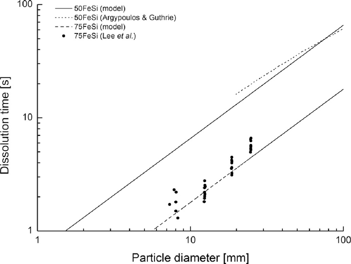
Given the amounts of FeSi typically fed into the vessel during the reduction stage, it is essential to consider related melting and dissolution behaviours. Experimental data for dissolution of 75FeSi particles is shown in Table 5. It is apparent that the dissolution time of FeSi is far shorter in the steel bath than it is in the slag bath. Simulations of fluid dynamics reported by Guthrie et al.⁷⁹⁾ suggest that FeSi additions do not surface but rather dissolve in the mixing zones located in the steel bath. Moreover, typical mixing times are estimated to be in the order of seconds due to vigorous argon stirring.⁸⁰⁾ Thus, it may safely be assumed that the limiting factor in the dissolution of additions in the steel melt is the melting of the material itself.

Table 5. Average dissolution times of 75FeSi particles at 1873 K.⁸¹⁾

Particle size [mm]	Average dissolution time in steel bath [s]	Average dissolution time in AOD slag [s]
25.4	5.6	136.9
19.1	3.7	87.4
12.7	2.2	47.1

Table 6. Parameters used for the dissolution model.

Property	75FeSi	50FeSi	SiMn	Steel scrap
Fe [wt-%]	23.8	50	10.3	99.0
Si [wt-%]	75	50	29.1	0.35
Mn [wt-%]	0	0	60.2	0.30
C [wt-%]	0.04	0.04	0.036	0.20
dp [m]	0.050	0.050	0.050	0.050
ρp [kg/m3]	280081)	610085)	612081)	775084)
Tm [K]	158981)	168385)	148881)	179384)
lm [J/kg]	144861781)	83946885)	49447381)	27200084)
λ [W/(m·K)]	2.9381)	9.6281)	4.18481)	–
λe [W/(m·K)]	9979.4×dp	5126.9×dp	1153.6×dp	1167.9×dp

In this model, the dissolution time of the particles is estimated in its simplest form by observing the melting time of a one-dimensional spherical form.⁴⁹⁾ An analytical solution for the melting time is given by:   

$${\tau }_{\text{m}}=\frac{{\text{d}}_{\text{p}}^2\rho \mathrm{\hspace{0.17em} }{\text{l}}_{\text{m}}}{8 {\lambda }_{\text{e}}({\text{T}}_{\text{Bath}}-{\text{T}}_{\text{m}})}$$(55)

where d_p is the particle size, T_m is the melting temperature, l_m is the latent heat of melting and λ_e is the effective heat conductivity of the particle. The corresponding average melting rate per mass unit is given by:   

$${\text{r}}_{\text{m}}=\frac{1}{{\tau }_{\text{m}}}$$(56)

However, it is known that when a cold alloy particle is added to the melt, an iron shell is formed around the particle surface, causing complex melting behaviour.⁸²⁾ In order to take this into account, effective heat conductivities were used and fitted to literature data on dissolution times of 75FeSi,⁸¹⁾ 50FeSi,⁸³⁾ SiMn⁸¹⁾ and steel scrap⁸⁴⁾ in a steel bath. All the relevant values used in this sub-model are presented in Table 6.

For particle sizes 10–50 mm, a good agreement with experimental results was achieved by assuming a linear dependency of effective heat conductivity from particle size (Figs. 4–5). The effective heat conductivities were substantially higher than the measured thermal conductivities as they include the effect of the exothermic reactions with the solid iron steel shell.⁸¹⁾

The temperature of the steel bath is updated upon additions according to the following equation:   

$${\text{T}}_{\text{Bath}}^{\text{New}}={\text{T}}_{\text{Bath}}-\frac{{\text{m}}_{\text{a}}}{{\text{m}}_{\text{a}}+{\text{m}}_{\text{Bath}}}\left(\left({\text{T}}_{\text{Bath}}-{\text{T}}_{\text{a}}\right)+\frac{{\text{l}}_{\text{m}}+\Delta {\text{h}}_{\text{dis}}}{{\text{c}}_{\text{p},\mathrm{\hspace{0.17em} }\text{L}}}\right)$$(57)

where ${\text{T}}_{\text{Bath}}^{\text{New}}$ is the updated bath temperature, m_a is the amount of molten addition per time step, T_a is the initial temperature of the addition and Δh_dis is the specific heat of dissolution from pure species to the Henrian standard state (1 mol-%). It should be noted here that the temperature of the top slag is updated likewise upon additions of slag formers.

Fig. 4.

Comparison of calculated and experimental^81,83) dissolution times of 75FeSi and 50FeSi particles in steel bath at 1873 K.

Fig. 5.

Comparison of calculated and experimental^81,84) dissolution times of SiMn (1873 K) and steel scrap particles (1923 K) in steel bath.

3.8. Numerical Solution Method

The objective of the numerical solution method is to solve the thermodynamic equilibrium and the set of conservation equations for mass and heat for each time step. Mass transfer coefficients, droplet size and droplet formation rate are held constant during each time step. In the first iteration cycle, the thermodynamic equilibrium and conservation of mass are solved simultaneously, while temperature is held constant in order to improve numerical stability. This does not cause any significant modelling error when small time steps are used.

In total, the conservation of mass in the system is defined by 45 equations: 21 equations for conservation of species in the surface element, 21 equations for conservation of species in the bulk phases and 3 equations for conservation of total mass in the steel bath, plume and the top slag, respectively. Contrary to the Newton-like method applied in the plume zone, the full Newton’s method was applied for numerical solution in the reduction model. This algorithm can be expressed as follows:   

$$\left[\text{J}\right]\times \left[\mathrm{\Delta }{\text{x}}_{\text{i}}\right]=\left[{\text{f}}_{\text{i}}\right]$$(58)

where [J] is the Jacobian matrix, [Δx_i] is the correction vector and [f_i] is the residual vector.

Fig. 6.

Flow sheet for the numerical solution of the surface element.

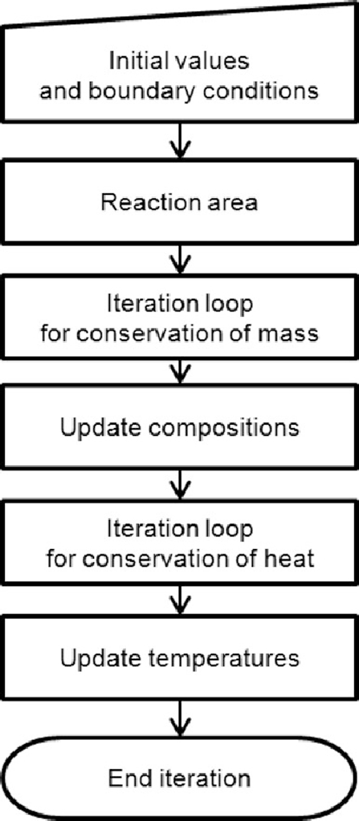
Figure 6 illustrates the flow sheet for the numerical solution of the surface element. The iteration loop starts with the calculation of a residual vector with the initial values. The Jacobian matrix is formed of differentiates with respect to all relevant species and masses, as illustrated below:   

$$\left[\begin{array}{ccc}\frac{\partial {\text{f}}_1}{\partial {\text{x}}_1}& \dots & \frac{\partial {\text{f}}_1}{\partial {\text{x}}_{45}}\\ ⋮& \ddots & ⋮\\ \frac{\partial {\text{f}}_{45}}{\partial {\text{x}}_1}& \dots & \frac{\partial {\text{f}}_{45}}{\partial {\text{x}}_{45}}\end{array}\right]\times \left[\begin{array}{c}\mathrm{\Delta }{\text{x}}_1\\ ⋮\\ \mathrm{\Delta }{\text{x}}_{45}\end{array}\right]=\left[\begin{array}{c}{\text{f}}_1\\ ⋮\\ {\text{f}}_{45}\end{array}\right]$$(59)

Numerical solution is achieved, when the residual vector approaches zero with a predefined accuracy. In the second iteration cycle, conservation of heat is solved likewise by the full Newton method. The governing equations are the conservation of heat at the interface and in the steel bath, in the top slag and in the plume gas, respectively. Under-relaxation factors are used in both solvers for increasing stability.

4. Results and Conclusion

Although numerous mathematical models have been proposed for modelling the decarburisation stage, the reduction stage has received much less attention. The model derived in this paper is a systematic attempt to construct a mathematical model for describing the dominating reaction phenomena during the reduction stage and also an extension to the previous model derived for side-blowing operation.

From a modelling perspective, a surface element with zero thickness is used to represent the reaction interface through which all reactions are assumed to occur. More specifically, an approach based on the law of mass action has been applied here for the simultaneous solution of the thermodynamic equilibrium of species and the governing masstransfer onto the reaction interface. Thermodynamic submodels have been employed for considering the activities of metal and slag species.

In this model, it was assumed that the reactions between emulsified slag droplets and the steel bath account for the dominating rate phenomena during the reduction stage. Hence the reaction interface consists of the total surface area of the emulsified droplets residing in the steel bath at a given moment. The effects of various physical parameters on the emulsification phenomena, including viscosity and density of steel and slag phases, have been taken into account.

The graphical user interface of the converter model has been updated to include relevant user functions for the mathematical model for the reduction stage. The user interface allows the addition of scrap, reductants, slag formers and fluxes and considers different feed rates for each batch of additions. In addition, a simple melting model is employed for describing the melting time of 75FeSi, 50FeSi, SiMn and scrap in the steel bath. Validation of the reaction model proposed in this paper is discussed thoroughly in Part II.⁸⁶⁾

Nomenclature

Symbols

A: Surface area [m²]

C_d: Drag coefficient

c_p: Specific thermal capacity [J/(kg·K)]

D: Diffusion coefficient [m²/s]

d: Diameter [m]

F: Force [N]

f: Conservation equation

g: Standard gravity [9.81 m/s²]

h: Mass transfer coefficient [m/s]

h: Specific enthalpy [J/kg]

K_eq: Equilibrium constant

k_f: Forward reaction rate constant

M: Molar mass [g/mol]

p: Partial pressure [Pa]

q: Heat flux [W/m²]

R: Universal gas constant

r_m: Melting rate [1/s]

Re: Reynolds number

R″: Reaction rate vector [kg/(m²·s)]

T: Temperature [K]

T_m: Melting temperature [K]

t_res: Residence time of slag droplets [s]

S: Molar entropy [J/mol·K]

u: Velocity [m/s]

u_i: Interfacial velocity [m/s]

$\overline{\text{V}}$ : Partial molar volume [m³/mol]

x: Mole fraction

y: Mass fraction

[Δx]: Correction vector

[J]: Jacobian matrix

 

Indices

a: Addition

B: Buoyancy

b: Bubble

dis: Dissolution

D: Slag droplet

D: Drag

G: Gas phase

G: Gravity

Bath: Steel bath (CSTR)

i: Species i

j: Species j

k: Species k

k: Reaction k

L: Liquid phase

S: Slag phase

s: Slip

SE: Surface element

Slag: Slag zone

p: Particle

Plume: Plume zone (PFR)

 

Greek symbols

α: Heat transfer coefficient [W/(m2·K)]

α: Interfacial angle [°]

Γ: Binary phase indicator

γ: Activity coefficient

ΔG: Change of reaction in Gibbs free energy [J/mol]

ΔH: Enthalpy of reaction [J/mol]

ΔS: Entropy of reaction [J/(mol·K)]

ε: 1^st order interaction parameter

η: Dynamic viscosity [Pa·s]

λ: Thermal conductivity [W/(m·K)]

λ_e: Effective heat conductivity [W/(m·K)]

ν_{i, k}: Stoichiometric coefficient of species i in reaction k, mole basis

${\overline{\nu }}_{\text{i},\mathrm{\hspace{0.17em} }\text{k}}$ : Stoichiometric coefficient of species i in reaction k, mass basis

π: Mathematical constant

ρ: Density [kg/m³]

σ: Interfacial tension [N/m]

τ_m: Melting time [s]

τ_r: Characteristic relaxation time [s]

Φ: Heat loss rate [W]

Acknowledgements

This research is a part of the Energy Efficiency & Lifecycle Efficient Metal Processes (ELEMET), a research program coordinated by the Finnish Metals and Engineering Competence Cluster (FIMECC). Outokumpu Stainless Oy, Finnish Funding Agency for Technology and Innovation (TEKES), Graduate School in Chemical Engineering (GSCE) and Academy of Finland (projects 258319 and 26495) are gratefully acknowledged for funding this work.

The authors would like to thank Dr Paavo Hooli, Mr Pentti Kupari and Mr Veikko Juntunen from Outokumpu Stainless Oy for their support and productive discussions regarding the paper. In addition, Mr Tommi Kokkonen, Mr Aki Kärnä and Mr Tuomas Alatarvas are acknowledged for their support. Dr John Braidwood and Mr Aaron Bergdahl are acknowledged for revising the language of this paper.

References

• 1)   W. A.  Krivsky: Metall. Trans., 4 (1973), 1439.
• 2)   E.-P.  Heikkinen and  T.  Fabritius:  M.  Nusheh, H. G. Ahuett and  A.  Arrambide: Recent Researches in Metallurgical Engineering - From Extraction to Forming, InTech, Rijeka, Croatia, (2012), 65.
• 3)   R. J.  Fruehan: Ironmaking Steelmaking, 3 (1976), 153.
• 4)   J.  Reichel and  J.  Szekely: Iron Steelmaker, 22 (1995), 41.
• 5)   M.  Järvinen,  A.  Kärnä and  T.  Fabritius: Steel Res. Int., 80 (2009), 431.
• 6)   M. P.  Järvinen,  S.  Pisilä,  A.  Kärnä,  T.  Ikäheimonen,  P.  Kupari and  T.  Fabritius: Steel Res. Int., 82 (2011), 638.
• 7)   S. E.  Pisilä,  M. P.  Järvinen,  A.  Kärnä,  T.  Ikäheimonen,  T.  Fabritius and  P.  Kupari: Steel Res. Int., 82 (2011), 650.
• 8)   S.  Asai and  J.  Szekely: Metall. Trans., 5 (1974), 651.
• 9)   J.  Szekely and  S.  Asai: Metall. Trans., 5 (1974), 1573.
• 10)   R. J.  Fruehan: Metall. Trans. B, 6 (1975), 573.
• 11)   R. J.  Fruehan: Metall. Trans. B, 8 (1977), 429.
• 12)   T.  Ohno and  T.  Nishida: Tetsu-to-Hagané, 63 (1977), 2094.
• 13)   T.  DebRoy and  D. G. C.  Robertson: Ironmaking Steelmaking, 5 (1978), 198.
• 14)   T.  DebRoy,  D. G. C.  Robertson and  J. C. C.  Leach: Ironmaking Steelmaking, 5 (1978), 207.
• 15)   A. E.  Semin,  A. P.  Pavlenko,  T.  Andzhum and  E. A.  Shuklina: Steel USSR, 13 (1983), 95.
• 16)   T.  Tohge,  Y.  Fujita and  T.  Watanabe: Proc. of the 4th Process Technology Conf., Iron & Steel Society of AIME, Warrendale, PA, USA, (1984), 129.
• 17)   P.  Sjöberg: Doctoral thesis, Kungliga Tekniska högskolan, Stockholm, Sweden, (1994), 157.
• 18)   M.  Görnerup and  P.  Sjöberg: Ironmaking Steelmaking, 26 (1999), 58.
• 19)   J.-H.  Wei and  D.-P.  Zhu: Metall. Mater. Trans. B, 33 (2002), 111.
• 20)   J.-H.  Wei and  D.-P.  Zhu: Metall. Mater. Trans. B, 33 (2002), 121.
• 21)   H.-L.  Zhu,  J.-H.  Wei,  G.-M.  Shi,  J.-H.  Shu,  Q.-Y.  Jiang and  H.-B.  Chi: Steel Res. Int., 78 (2007), 305.
• 22)   G.-M.  Shi,  J.-H.  Wei,  H.-L.  Zhu,  J.-H.  Shu,  Q.-Y.  Jiang and  H.-B.  Chi: Steel Res. Int., 78 (2007), 311.
• 23)   J.-H.  Wei,  Y.  Cao,  H.-L.  Zhu and  H.-B.  Chi: ISIJ Int., 51 (2011), 365.
• 24)   N. Å. I.  Andersson: Doctoral thesis, Kungliga Tekniska högskolan, Stockholm, Sweden, (2012), 42.
• 25)   N. Å. I.  Andersson,  A.  Tilliander,  L. T. I.  Jonsson and  P. G.  Jönsson: Ironmaking Steelmaking, DOI: 10.1179/1743281212Y.0000000060.
• 26)   N. Å. I.  Andersson,  A.  Tilliander,  L. T. I.  Jonsson and  P. G.  Jönsson: Steel Res. Int., 83 (2012), 1039.
• 27)   N. Å. I.  Andersson,  A.  Tilliander,  L. T. I.  Jonsson and  P. G.  Jönsson: Steel Res. Int., 84 (2013), 169.
• 28)   P.  Ternstedt,  R.  Gyllenram,  J.  Bengtsson and  P. G.  Jönsson: The 6th European Oxygen Steelmaking Conf., Jernkontoret, Stockholm, Sweden, (2011), 1.
• 29)   M.  Engholm: Nord. Steel Min. Rev., 3 (2008), 125.
• 30)   J.  Riipi,  T.  Fabritius,  E.-P.  Heikkinen,  P.  Kupari and  A.  Kärnä: ISIJ Int., 49 (2009), 1468.
• 31)   S.  Asai: 100th and 101st Nishiyama Memorial Seminar, ISIJ, Tokyo, Japan, (1984), 67.
• 32)   J.  Mietz and  M.  Brühl: Steel Res., 61 (1990), 105.
• 33)   M. G.  Frohberg,  F.  Gerlach and  G.  Handschuh: Steel Res., 61 (1990), 151.
• 34)   J.  Mietz,  S.  Schneider and  F.  Oeters: Steel Res., 62 (1991), 1.
• 35)   J.  Mietz,  S.  Schneider and  F.  Oeters: Steel Res., 62 (1991), 10.
• 36)   T.  Wei and  F.  Oeters: Steel Res., 63 (1992), 60.
• 37)   Z.  Lin and  R. I. L.  Guthrie: Metall. Mater. Trans. B, 25 (1994), 855.
• 38)   A. W.  Cramb,  Y.  Chung,  J.  Harman,  A.  Sharan and  I.  Jimbo: Iron Steelmaker, 24 (1997), 77.
• 39)   H.  Lachmund,  Y.  Xie,  T.  Buhles and  W.  Pluschkell: Steel Res., 74 (2003), 77.
• 40)   H.  Solhed,  L.  Jonsson and  P.  Jönsson: Steel Res. Int., 79 (2008), 348.
• 41)   P.  Sulasalmi,  A.  Kärnä,  T.  Fabritius and  J.  Savolainen: ISIJ Int., 49 (2009), 1661.
• 42)   J.  Savolainen,  T.  Fabritius and  O.  Mattila: ISIJ Int., 49 (2009), 29.
• 43)   M.  Görnerup and  A. K.  Lahiri: Ironmaking Steelmaking, 25 (1998), 317.
• 44)   M.  Görnerup and  A. K.  Lahiri: Ironmaking Steelmaking, 25 (1998), 382.
• 45)   T.  Nakasuga,  H.  Sun,  K.  Nakashima and  K.  Mori: ISIJ Int., 41 (2001), 937.
• 46)   T.  Nakasuga,  K.  Nakashima and  K.  Mori: ISIJ Int., 44 (2004), 665.
• 47)   F.  Oeters: Metallurgie der Stahlherstellung, Verlag Stahleisen mbH, Düsseldorf, Germany, (1989), 503.
• 48)   Y.  Okabe,  I.  Tajima and  K.  Ito: Metall. Mater. Trans. B, 29 (1998), 131.
• 49)   M.  Järvinen,  A.  Kärnä,  S.  Ollila and  T.  Fabritius: 4th Int. Conf. on Process Development in Iron and Steelmaking, Swerea MEFOS, Luleå, Sweden, (2012), 79.
• 50)   A. H.  Castillejos,  M. E.  Salcudean and  J. K.  Brimacombe: Metall. Trans. B, 20 (1989), 603.
• 51)   A.  Kärnä,  T.  Fabritius and  L.  Hekkala: Flow model for the AOD converter (in Finnish). Report 327. University of Oulu, Laboratory of Process Metallurgy, Oulu, Finland, (2007), 47.
• 52)   K.  Yonezawa and  K.  Schwerdtfeger: Metall. Mater. Trans. B, 31 (2000), 461.
• 53)   P. R.  Scheller: Doctoral thesis, Rheinisch-Westfälische Technische Hochschule Aachen, Aachen, Germany, (1985), 88.
• 54)   K.  Yonezawa and  K.  Schwerdtfeger: Metall. Mater. Trans. B, 30 (1999), 655.
• 55)   B. J.  Keene and  K. C.  Mills: Verein Deutscher Eisenhüttenleute: Slag Atlas, 2nd ed., Verlag Stahleisen GmbH, Düsseldorf, Germany, (1995), 313.
• 56)   T.  Fabritius,  J.  Riipi,  M.  Järvinen,  O.  Mattila,  E.-P.  Heikkinen,  A.  Kärnä,  J.  Kurikkala,  P.  Sulasalmi and  J.  Härkki: ISIJ Int., 50 (2010), 797.
• 57)   L.  Forsbacka,  L.  Holappa,  A.  Kondratiev and  E.  Jak: Steel Res. Int., 78 (2007), 676.
• 58)   G.  Urbain: Steel Res., 58 (1987), 111.
• 59)   R.  Higbie: Trans. Am. Inst. Chem. Eng., 31 (1935), 365.
• 60)   A. K.  Lahiri: Fundamentals of Metallurgy, ed. by  S.  Seetharaman, Woolhead Publishing Limited, Cambridge, UK, (2005), 178.
• 61)   R.  Clift,  J. R.  Grace and  M. E.  Weber: Bubbles, Drops and Particles, Academic Press, New York, USA, (1978), 380.
• 62)   J. H.  Seinfeld and  S. N.  Pandis: Atmospheric Chemistry and Physics: From Air Pollution to Climate Change, John Wiley & Sons Ltd., New York, USA, (1998), 1326.
• 63)   M.  Iguchi,  H.  Kawabata,  K.  Nakajima and  Z.  Morita: Metall. Mater. Trans. B, 26 (1995), 67.
• 64)   A.  Tilliander,  T. L. I.  Jonsson and  P. G.  Jönsson: ISIJ Int., 44 (2004), 326.
• 65)   B.  Deo and  R.  Boom: Fundamentals of Steelmaking Metallurgy, Prentice Hall International, Hertfordshire, UK, (1993), 300.
• 66)   H. D.  Mendelson: Am. Inst. Chem. Eng. J., 13 (1967), 250.
• 67)  HSC Chemistry for Windows ver. 6.0., Outokumpu Research Oy, Pori, Finland, (2006).
• 68)   G. K.  Sigworth and  J. F.  Elliott: Met. Sci., 8 (1974), 298.
• 69)   A. D.  Pelton and  C. W.  Bale: Metall. Trans. A, 17 (1986), 1211.
• 70)   L. S.  Darken: Trans. Met. Soc. AIME, 239 (1967), 80.
• 71)   L. S.  Darken: Trans. Met. Soc. AIME, 239 (1967), 90.
• 72)   C. W.  Wagner: Handbuch der Metallphysik, ed. by  G.  Masing, Akademische Verlagsgesellschaft Becker & Erler, Leipzig, Germany, (1940).
• 73)   C. H. P.  Lupis and  J. E.  Elliott: Acta Metall., 14 (1966), 529.
• 74)   A. V.  Alpatov and  S. N.  Paderin: Russ. Metall., 2010 (2010), 557.
• 75)   S.  Ueno,  Y.  Waseda,  T.  Jacob K. and  S.  Tamaki: Steel Res., 59 (1988), 474.
• 76)   W. E.  Slye and  R. J.  Fruehan: 57th Electric Furnace Conf., Iron & Steel Society of AIME, Warrendale, PA, USA, (1999), 401.
• 77)   K. V.  Malyutin and  S. N.  Paderin: Russ. Metall., 2007 (2007), 545.
• 78)   J.-H.  Wei: Chin. J. Met. Sci. Technol., 5 (1989), 235.
• 79)   R. I. L.  Guthrie,  M.  Isac and  Z.-H.  Lin: Ironmaking Steelmaking, 32 (2005), 133.
• 80)   P.  Ternstedt,  A.  Tilliander,  P. G.  Jönsson and  M.  Iguchi: ISIJ Int., 50 (2010), 663.
• 81)   Y. E.  Lee,  H.  Berg and  B.  Jensen: Ironmaking Steelmaking, 22 (1995), 486.
• 82)   L.  Zhang and  F.  Oeters: Melting and Mixing of Alloying Agents in Steel Melts. Methods of Mathematical Modelling. Verlag Stahleisen GmbH, Düsseldorf, Germany, (2006), 111.
• 83)   S. A.  Argyropoulos and  R. I. L.  Guthrie: Can. Metall. Q., 18 (1979), 267.
• 84)   J.  Li,  G.  Brooks and  N.  Provatas: Metall. Mater. Trans. B, 36 (2005), 293.
• 85)   I.  Barin: Thermochemical Data of Pure Substances, Part I, VCH Verlagsgesellschaft mbH, Weinheim, Germany, (1989), 816.
• 86)   V.-V.  Visuri,  M.  Järvinen,  J.  Savolainen,  P.  Sulasalmi,  E.-P.  Heikkinen and  T.  Fabritius: ISIJ Int., 53 (2013), 613.