Regular Article
Analysis of Melt Flow in Metallurgical Vessels of Steelmaking Processes
2013 Volume 53 Issue 4 Pages 622-628
Details
2013 Volume 53 Issue 4 Pages 622-628
Control of melt flow in steelmaking processes is important for technology optimization and product quality. To overcome the difficulty of making measurements in actual steelmaking vessels (furnace, ladle, tundish, or mold), both physical modeling (water models) and CFD simulations have been used extensively for melt flow visualization. However, it is not easy to interpret the results of either type of model study, because it is difficult to determine which flow pattern is best by only visual inspection. In this article, a new approach is proposed for the analysis of the melt flow in metallurgical vessels after obtaining residence time distributions from CFD simulation or physical experiments (RTDCFD or RTDmodel). In this analysis the melt flow is assumed to be in a combined reactor (CR) system consisting of a combination of three basic unit reactors: “plug flow”, “perfect mixer”, and “recirculated volume”. An inverse simulation is used to define the volumes of the unit reactors and the melt flow rate between them by fitting the RTDCR curve to the RTDCFD or RTDmodel curves. The effectiveness of the suggested approach is demonstrated for tundish applications; however, it could also be used for melt flow analysis in other steelmaking processes.
CFD simulation and physical modeling of liquid metal processing are both carried out in order to achieve several major objectives, which can be classified into three levels:
Level 1: to understand the process, for example, the melt flow pattern and/or chemical reaction kinetics in metallurgical vessels;
Level 2: to optimize existing and design new processes and equipment, for example, optimize the geometry of an industrial tundish;
Level 3: to control the entire steelmaking process on-line, when several models need to be integrated in a fast-working algorithm communicating with sensors and process control devices.
Knowledge of the melt flow phenomena is essential to meet these objectives. For example, in the continuous casting of steel, the modern-day tundish is designed with various metallurgical operations in mind, such as inclusion separation, alloy trimming and thermal and chemical homogenization. A broad review of the methods used to understand the nature of melt flow in the ladle and the tundish (Level 1 objectives) can be found elsewhere.1,2,3) However CFD simulation alone is not so effective in achieving Level 2 objectives because it is not easy to determine which flow pattern is best, simply by visual inspection. The complexity of commercial CFD codes and the time involved in running simulations also make it impractical to apply CFD simulation on-line to pursue Level 3 objectives.
Figure 1 schematically illustrates the capabilities of the different methods to meet Level 1 – Level 3 objectives. The method capabilities are ranked as high (H), low (L) or not applicable (N). For example, physical modeling has high capability for analysis of such process phenomena as melt flow, inclusion separation (Level 1 objectives), less capability for novel process design and optimization (Level 2 objectives) and is not applicable to on-line process control (the Level 3 objective). Another example is non-dimensional analysis which is used as a tool to achieve similarity between water modeling experiments and the industrial process.4) This method has limited capability to evaluate the melt flow and inclusion separation in metallurgical vessels, and is not applicable for new design and on-line process control.

Capabilities of experimental and modeling methods to solve different objectives in liquid metal processing (tundish application example).
The combined reactors approach was originally developed by Levenspiel5) and Kafarov6) to analyze chemical engineering processes as a set of interconnected unit reactors such as the Continuous-Stirred-Tank Reactor (CSTR) and Plug Flow Reactor (PF). By solving the mass conservation equations, the flow can be characterized in the terms of the mean residence time (RT) and the residence-time distribution (RTD). The RTD curve in an actual process or physical model is obtained by short time dye injection into the in-flow stream and measuring the dye concentration in the out-flow stream from the system. The combined reactors approach was adopted to describe the melt flow in metallurgical furnaces by Thermelis and Szekely.7) Later it was used by Sahai and Emi8) for a continuous casting tundish by dividing the vessel into unit reactors, based on the measured RTD curve.
In the first part of the article, the possible discrepancies of combined reactor approach are demonstrated using the example of melt flow in tundishes with different flow control devices. To solve this problem, a new approach of melt flow modeling in metallurgical vessels was developed. The suggested method is based on CFD simulation followed by inverse modeling of an assumed combined reactor (CR) architecture to achieve a good match between the RTDCR and the RTDCFD by varying the volume of the unit reactors and the flow rates between them. This approach has a medium/high capability to solve the different objectives in liquid metal processes shown in Fig. 1.
The single-strand tundish of 14 metric ton liquid steel capacity was modeled. The tundish had a trapezoidal shape with 10 degree vertical walls incline and 3 m long, 1 m wide and 0.8 m melt level. The melt flow rate was varied from 2 t/min (slow) to 2.6 t/min (medium) and to 3.2 t/min (high). This gave 446, 340 and 270 seconds for the mean RT values respectively. The tundish had a submerged entry nozzle (SEN) of 250 mm OD, and 150 mm ID submerged 300 mm into the melt, and a 200 mm OD stopper rod above a 70 mm diameter exit nozzle. Three cases were compared: no flow control devices (Fig. 2(a)), with flow control devices (Fig. 2(b)), and with a bottom Ar mixing plug (6.7 m3/h flow rate) under the SEN in a design similar to Fig. 2(a).
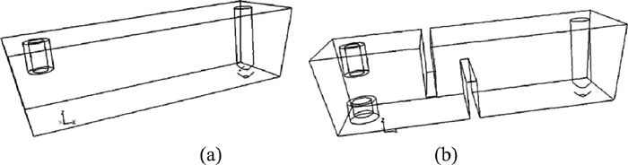
Tundish design: a) no flow control and b) with flow control devices.
CFD FLUENT 12.0 software was used to solve isothermal transient turbulent melt flow; species transport was included to allow the derivation of the RTD curve. Discrete second phase model was also used for tracking non-metallic inclusions. The Euler-Lagrange approach was used in discrete phase model.9) The fluid phase is treated as a continuum by solving the Navier-Stokes equations, while the dispersed phase is solved by tracking a large number of particles through the calculated flow field. The trajectory of a discrete phase particle was predicted by integrating the force balance on the particle. This force balance equates the particle inertia with the drag forces and gravity acting on the particle. In addition, a multiphase model was used in the Ar-mixing case. The main computational details are given in Table 1 and further information can be found in the FLUENT manual.9) The isothermal melt flow was adequate to demonstrate the differences in the melt flow in the studied cases.
| Process | Model | Specific details |
|---|---|---|
| Melt flow | Transient turbulent | -standard k-epsilon |
| Ar-mixing | Multiphase | -VOF, implicit |
| RTD curve | Species Transport | -volumetric reaction |
| Inclusion tracking | Discrete Phase | -random walk unsteady particle tracking -surface injection (inlet) -particle boundary conditions: inlet-injection; top-trap: outlet-escape: other walls-reflect |
Transient turbulent melt flow was solved to obtain a stable flow pattern, controlled by an average volume velocity. A rapid (5 seconds) injection of specie with the melt properties (viscosity and density) through the SEN was used in obtaining the RTD curve. A similar surface location of inert particle injection (discrete phase) was used to track nonmetallic inclusions of medium (20 µm) and large size (100 µm) with a 3.5 g/cm3 density. Particle boundary conditions included: injection of spherical particles through the inlet, particles trap by the top melt surface (lost from the calculation at the point of particle impact with the boundary), and particles escape through the outlet. The number of particles in domain, trapped by top surface, and vent through outlet was reported at each time step. Solution of the discrete phase implies integration in time of the force balance on the particle.
CFD modeling showed that there was a substantial difference in the general flow patterns between the three tundish cases. This could be observed in the vector velocity distribution in the central vertical plane:
- poorly organized flow in the tundish without flow control devices (Fig. 3(a))
- mostly sequential flow with two easily recognized recirculation zones in the tundish with flow control devices (Fig. 4(a)), and
- a vertical melt stream generated by Ar-bubbles near the SEN with a poorly organized flow pattern in other parts of the tundish volume (Fig. 5(a)).

Tundish without flow control devices: a) vectors of melt velocity in the central plane and b) – e) tracer concentration in the central plane after 5, 100, 200 and 300 seconds of injection (0.015; 0.3; 0.6; and 0.9 fraction of mean RT).
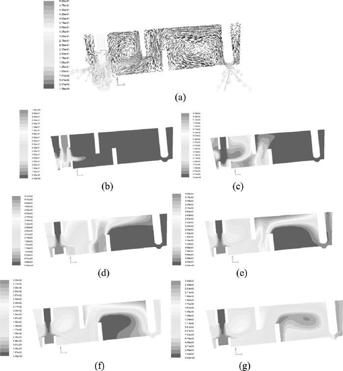
Tundish with flow control devices: a) vectors of melt velocity in the central plane and b) – g) tracer concentration in the central plane after 5, 20, 50, 75, 100 and 170 seconds of injection (0.015, 0.06, 0.15, 0.22, and 0.3 fraction of mean RT).
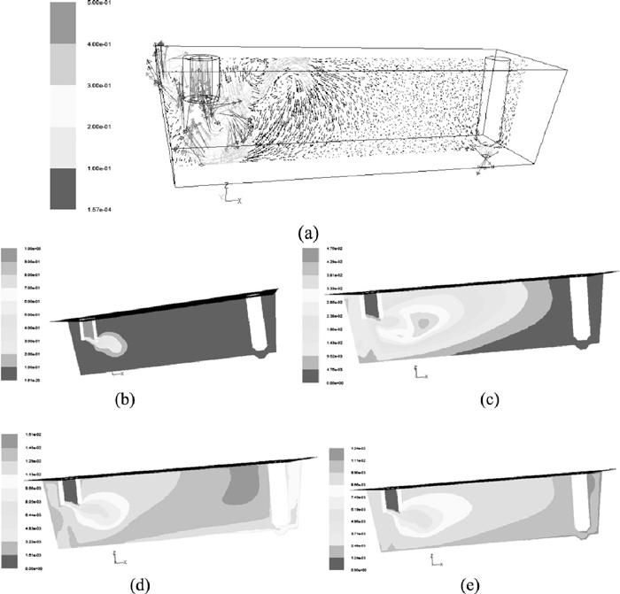
Tundish with Ar-mixing: a) vectors of melt velocity in the central plane and b) – e) tracer concentration in the central plane after 5, 20, 75, and 170 seconds of injection (0.015, 0.06, 0.22, and 0.5 fraction of mean RT).
The different flow patterns in these three cases provided significant differences in the shape of the RTD curves plotted in terms of dimensionless concentration C (ratio of injection dose to tundish volume) and time θ (ratio of process time to mean residence time). The RTD curve for the tundish without flow control devices has a smooth bell-like shape. Flow control devices deformed the shape of the RTD curve, increasing the peak value and shortened the time of its occurrence. Ar-mixing also moved the RTD curve to the left and significantly shortened the time when the tracer first reached the outlet; however it had no effect on the maximum value (Fig. 6(a)). Changing the melt flow rate had a minimal effect on the RTD curves (Figs. 6(b) and 6(c)). The three modeled tundish cases demonstrated large differences in the melt flow pattern reflected in the shape of the RTD curves.

The RTD curves for: a) three different tundish designs at medium flow rate, b) the tundish without flow control and c) the tundish with flow control devices at different flow rates.
As mentioned earlier process flow modeling based on the combined reactors approach was first carried out by Levenspiel5) and Kafarov6) in the field of chemical engineering. Later this concept was adopted by Themelis and Szekely7) and Sahai and Emi8) for the description of flow in other technologies including metallurgical processes. In metallurgical vessels, a tundish for example, the different zones are not distinct or easily defined which is a challenge to the design an adequate combined reactors architecture.
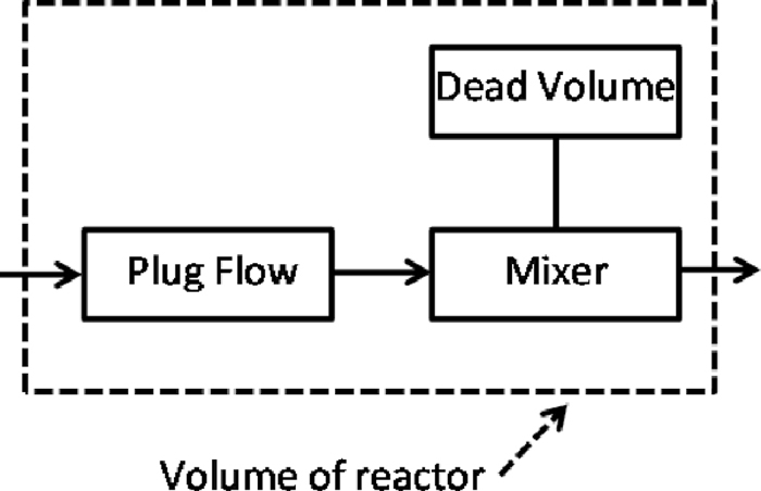
3.1. Previous ApproachIn the previous approach,8) the a priori assumed architecture of combined reactors model consists of a combination of three reactors: a “plug flow” reactor, an “ideal mixer” and, a so called, “dead volume” (Fig. 7). It was assumed that, the volumes of these three reactors can be calculated from the RTD curve obtained from physical modeling or CFD simulation. However the specific parameters, including flow rates between the reactors, were no defined. The rules used to calculate the volumes of these reactors were that:8)
- the plug zone volume is given by the delay time in the appearance of tracer (tp),
- the dead volume is determined by the fraction of the tracer that appears after θ = 2, and
- the mixer volume is the total volume minus the plug and dead volumes.
Combined reactors architecture used in previous approach.8)
In this study, these rules were applied to determine the volumes of the unit reactors for the different tundish designs described above (Table 2). The values of the reactor volumes using these rules are in reasonable qualitative agreement with the flow pattern obtained from CFD modeling (Figs. 3(a), 4(a) and 5(a)). The tundish with flow control device provided the largest plug flow volume, while Ar-mixing minimized plug flow. The tundish with flow control devices had the largest dead volume.
| Reactor | Tundish design | |||
|---|---|---|---|---|
| Without flow control | With flow control devices | Ar-mixing | ||
| Plug | 10.1 | 19.9 | 5.4 | |
| Mixing | 81.9 | 66.8 | 83.7 | |
| Dead zone | 8.0 | 13.3 | 10.9 | |
Mass conservation equations were implemented in EXCEL spreadsheets for the case of the tundish without flow control devices (Fig. 2(a)). Because there is no real “dead zone” with zero flow rate in metallurgical vessel, the term “recirculated volume” (RV) was used in this article instead of “dead volume”. In the first type of combined reactors (insert in Fig. 8(a)), plug flow reactor was followed by a mixer directly connected to RV reactor. In the second type of combined reactors (insert in Fig. 8(b)), RV reactor was bypass-connected to the mixer. There is important to note that solving mass conservation equations required the value of flow rate between the mixer and RV. The calculated volumes (Table 2) and assumed combined reactor (CR) architectures according to the inserts in Fig. 8 were used to calculate the RTDCR curves. It can be seen that there was no agreement between the RTDCFD curve used as input for calculation of volumes of the reactor and calculated RTDCR curves at any combination of variables.
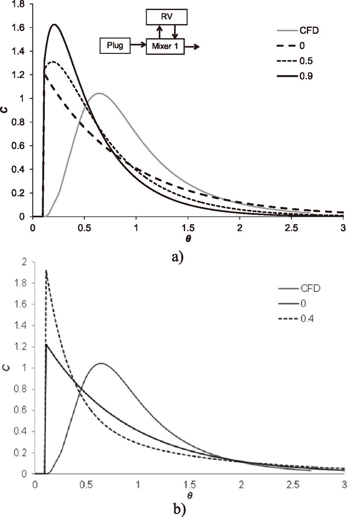
Tundish without flow control devices: comparison of CFD simulated RTDCFD curves with RTDCR curves obtained from the previous combined reactor approach. Numbers on graphs show the fraction of the melt flow through the recirculated volumes.
It can be concluded that the applicability of the previous approach, and the rules to calculate the reactor volumes from CFD simulated RTDCFD curves, are not correct when the values derived from the rules and the presumed architecture are put to the mass conservation simulation test.
3.2. Combined Reactor Design Based on Inverse OptimizationA novel strategy of combined reactor design is suggested below for the achievement of a reasonable similarity between RTDCFD or RTDmodeling curves with generated RTDCR curves from combined reactor models. To represent the melt flow patterns in the tundish, the suggested combined reactor architectures consist of one plug flow reactor and two or three ideal (or perfect) mixers, each loop-connected with recirculated volumes (RV) (Fig. 9). Preliminary mass conservation simulation tests showed that these architectures are more suitable when compared to the set of unit reactors (Fig. 7) used in the previous approach, and also better represent the fluid flow pattern in the tundish.
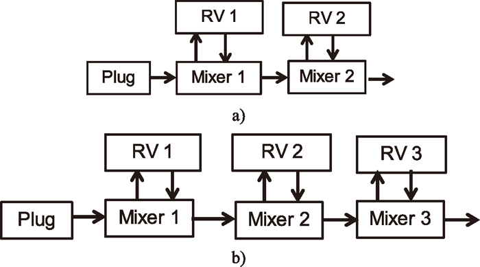
Possible architectures of combined reactors, with a plug flow reactor, and (a) two, or (b) three mixers in series with recirculated volume (RV) loops.
In the combined reactors architectures, the several parameters, such as the reactor volumes and the flow rates in mixers - RV loops, need to be defined. This problem is difficult to solve analytically; however, it can be solved numerically. The method used to derive the combined reactors model to represent CFD (or experimental) RTD curves was as follows:
- (i) defining the architecture of the combined reactors;
- (ii) building a combined reactor mass conservation flow sheet with calculation of the RTDCR curve for an arbitrary set of parameters of reactor volumes and flow rates;
- (iii) finding the values of these parameters by fitting the calculated RTDCR curve to the “true” RTDCFD curve by inverse optimization.
The flow process mass conservation (numerical integration) spreadsheet programs were developed for the different combined reactor architectures using Microsoft EXCEL. A function (φ) was minimized (Eq. (1)) with the built-in EXCEL Solver:
| (1) |
The method is illustrated for the three cases discussed earlier. It was found that in some cases the simpler architecture of combined reactor design with two mixers – RV loops provided a reasonable agreement between RTDCFD and RTDCR curves. However three mixers-RV loops gave better agreement.
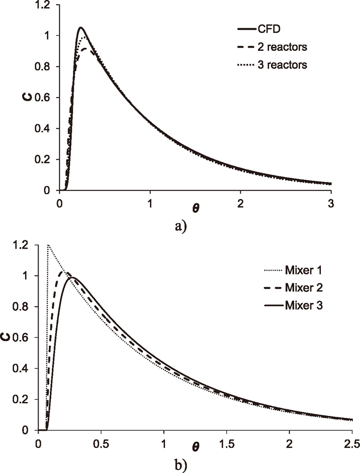
Tundish with no flow control devices. Figure 10 illustrates the RTDCR curves for two and three mixer – RV loops (indicated as 2 or 3 reactors in Fig. 9) in comparison to the “true” RTDCFD curve (indicated as CFD in Fig. 10) for the tundish without flow control devices. The three mixer design provided a significantly better agreement with a “true” CFD simulated RTDCFD curve when compared to single (Fig. 8) or double mixers. Inverse modeling delivered a combination of the variables (Table 3) which indicated that RV volumes are negligible and can be omitted. In this case, the combined reactors structure consisted of a small plug volume connected to three in-line ideal mixers. This is a reasonable combined reactor representation of the CFDvisualized flow pattern in the case of the tundish without flow control devices. It could be also characterized as a dispersed plug flow pattern.5)
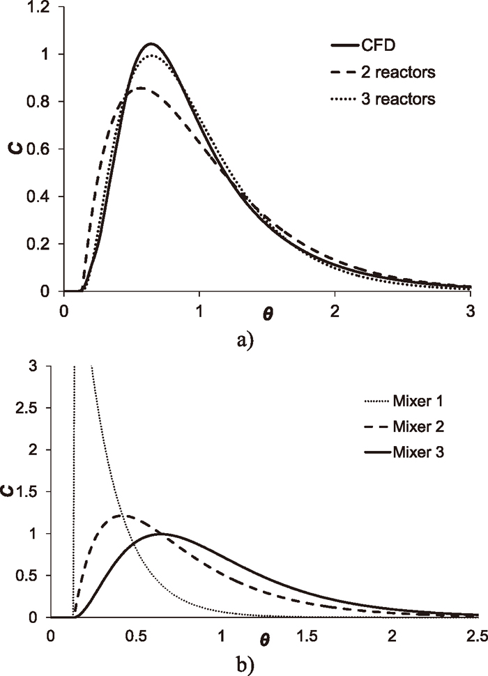
Tundish without flow control devices: (a) RTD curves from CFD model and combined reactors and (b) tracer concentration in the three sequentially connected reactors.
| Reactor volume, part from tundish | Flow rate ratio | ||||||||
|---|---|---|---|---|---|---|---|---|---|
| Plug | Mix 1 | RV 1 | Mix 2 | RV 2 | Mix 3 | RV 3 | Mix1-RV1 | Mix 2-RV2 | Mix 3-RV3 |
| 0.14 | 0.20 | – | 0.41 | 0.01 | 0.2 | 0.01 | – | 1.0 | 1.0 |
| Reactor volume, part from tundish | Flow rate ratio | ||||||||
|---|---|---|---|---|---|---|---|---|---|
| Plug | Mix 1 | RV 1 | Mix 2 | RV 2 | Mix 3 | RV 3 | Mix1-RV1 | Mix 2-RV2 | Mix 3-RV3 |
| 0.23 | 0.05 | – | 0.11 | 0.15 | 0.12 | 0.34 | – | 0.75 | 0.94 |
Tundish with flow control devices. Flow control devices significantly changed the melt flow pattern (Fig. 4(a)) and therefore the RTD curve (Fig. 6(a)). In this case, only the three mixer-RV loop architecture was in a reasonable agreement with CFD flow pattern (Fig. 11). The first loop had negligible RV volume however the two other loops had moderate recirculation. This combined reactors structure also could be observed from the CFD calculated vector velocity pattern (Fig. 6(a)).
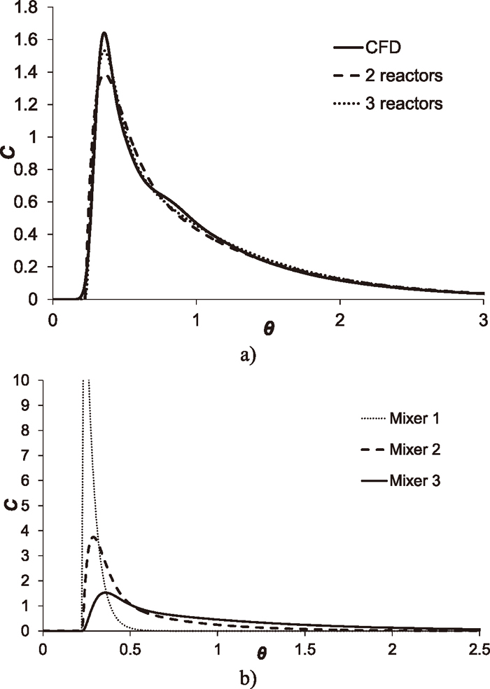
Tundish without flow control devices: (a) RTD curves from CFD model and combined reactors and (b) tracer concentration in the three sequentially connected mixers.
Tundish with Ar-stirring. Finally, the combined structure for Ar-stirred tundish consisted of a very small plug flow adjusted to the large well mixed volume with a small RV. Two more small recirculated loops were also predicted in this case (Fig. 12, Table 5).
Ar-stirred tundish: (a) RTD curves from CFD model and combined reactors and (b) tracer concentration in the three sequentially connected mixers.
| Reactor volume, part from tundish | Flow rate ratio | ||||||||
|---|---|---|---|---|---|---|---|---|---|
| Plug | Mix 1 | RV 1 | Mix 2 | RV 2 | Mix 3 | RV 3 | Mix1-RV1 | Mix 2-RV2 | Mix 3-RV3 |
| 0.07 | 0.81 | 0.01 | 0.02 | 0.04 | 0.04 | 0.01 | 2.1 | 7.1 | 1.2 |
CFD simulations and experimental observations showed the complicated flow patterns in the tundish and a possibility to re-organize this flow pattern by applying flow control devices and/or Ar-stirring. The described approach provided an opportunity to present the CFD modeled flow pattern as an optimized combination of unit reactors. Table 6 illustrates the precision of the suggested approach versus the previously published method for the three studied tundish designs.
| Tundish | Previous method | Combined approach | |
|---|---|---|---|
| 2 reactors | 3 reactors | ||
| No flow control | 102 | 9.8 | 0.8 |
| Flow control | 80 | 3.6 | 0.7 |
| Ar-mixing | 110 | 2.0 | 0.6 |
The formalization of melt flow in tundish using the suggested optimization of combined reactors can provide an important practical applications including:
- understanding how a particular tundish design works;
- tundish design optimization applying the several trials of CFD plus inversed simulations of combined reactors architecture and comparison of desired function (reactors volumes, flow rate, melt mixing and refining);
- the design of combined reactor models for the entire steel making process including different vessels.
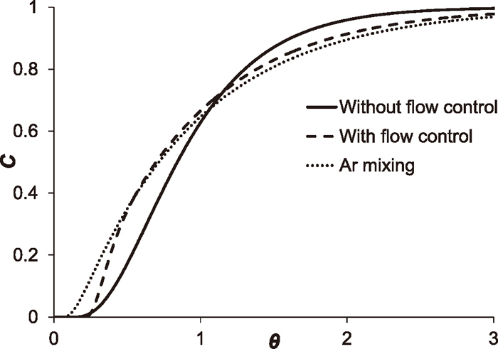
Additional studies are needed to determine the relationships between the melt flow pattern and the internal/external exogenous/endogenous processes (particle movements, processes occurring at the melt/slag and slag/gas interfaces, reaction kinetics, etc.). However, the suggested combined reactors could well be a useful method for solving these tasks. For example, it will allow us to predict steel chemistry variations during ladle change (Fig. 13). On this graph, zero represents the initial concentration and one the final composition for any given species.
Predicted outflow melt composition after chemistry change in SEN for different tundish design.
The complexity of understanding the different process interactions in the metallurgical vessel may be illustrated by taking the example of the effect of changing tundish design on non-metallic inclusion separation from the melt. The large (100 µm) and medium (20 µm) size non-metallic inclusions were introduced into the tundish through SEN for a short time (1 sec). It was assumed that particles will be trapped if they touch the top melt surface. Other possible mechanisms of particle removal were not discussed because they play a minor role for such size particles.10) Figure 14 shows the percentage of particles which were trapped by the top surface and leaving tundish with the melt. For large particles, Ar-mixing provided a more intensive rate of particle sorption by the top surface, and the tundish with flow control allowed later escape; however, the overall percentage of these large particles in an exit stream was low for all studied tundish designs. However, this was not true for the medium (20 µm) size particles and the tundish design had a significant effect on medium (20 µm) size particle behavior.
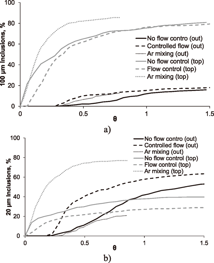
Evolution of injected 100 µm (a) 20 µm (b) inclusions in different tundish design.
A new approach is proposed for the analysis of the melt flow in metallurgical vessels by the inversed simulation of combined reactor architecture and parameters. The melt flow is assumed to be in a combined reactor consisting of a connected series of basic flow reactors including plug flow, perfect mixer, and recirculated volume. An arbitrary residence time distribution (RTDreactor) curve was obtained for this combined reactor by solving the mass conservation equations numerically. Then the volumes of the basic reactors and the melt flows between them were fitted to the RTDCFD curve derived from the CFD or water models by an inverse simulation.
The effectiveness of the suggested approach was demonstrated for tundish applications. Three different tundish designs (with and without flow control devices and Ar-stirred) were CFD simulated and showed the different behavior of RTDCFD curves. The suggested and existing approaches were applied to design and calculate combined reactors volumes and flow rate. It was shown that the existing method does not provide the flow rate values and there was no agreement between the RTDCFD and RTDreactor curves at any combination of the variables (reactor volume and flow rate). Based on the visualization of CFD flow patterns, the different combined reactor architectures were suggested and reactor parameters were calculated using inverse simulations. The precision of the suggested method was proven for different tundish designs. The suggested combined reactors can be a useful tool for solving melt flow problems in different liquid metal processing.