Modeling of Gas Metal Arc Welding Process Using an Analytically Determined Volumetric Heat Source

Abstract

High peak temperature and continuous deposition of electrode droplets in the weld puddle inhibit real-time monitoring of thermal cycles and bead dimensions in gas metal arc welding. A three-dimensional numerical heat transfer model is presented here to compute temperature field and bead dimensions considering a volumetric heat source to account for the transfer of arc energy into the weld pool. The heat source dimensions are analytically estimated as function of welding conditions and original joint geometry. The deposition of electrode material is modeled using deactivation and activation of discrete elements in a presumed V-groove joint geometry. The computed values of bead dimensions and thermal cycles are validated with the corresponding measured results. A comparison of the analytically estimated heat source dimensions and the corresponding numerically computed bead dimensions indicate that the former could rightly serve as the basis for conduction heat transfer based models of gas metal arc welding process.

1. Introduction

In recent times, numerical simulation models have become an indispensable tool for a priori quantitative understanding of the influence of welding conditions on weld thermal cycles, bead dimensions, weld joint mechanical properties and, distortion and residual stresses.^1,2,3,4) Although several efforts are published to simulate autogenous fusion welding processes, similar models that can also consider the electrode deposition such as in gas metal arc welding process (GMAW) and submerged arc welding (SAW) are only a few.^{5,6,7,8,9,10,11,12,13,14,15,16,17,18)} The convective heat transport based have remained as a route to realize heat transfer and fluid flow in weld pool, and the resulting weld pool profile. ^{8,9,10,11,12,13,18)} The conduction heat transfer based models for GMAW and SAW processes have also remained an effective recourse because of their computational simplicity, flexibility to consider wide-ranging weld joint geometry, and quick adoptability in several numerical analysis software that are widely available.^{5,6,7,14,15,16,17)} In contrast, the analytical heat transfer models to simulate GMAW process could consider simple joint geometry and constant material properties that usually inhibited accurate prediction of temperature field within the weld pool.^19,20) The majority of the conduction heat transfer based numerical models considered a volumetric heat source to account for the transfer of arc energy in the weld pool and, the heat source dimensions are determined either arbitrarily or based on the measured final weld dimensions that had restricted the predictive capability of these models. An effective alternative will be to develop a methodology to estimate the heat source dimensions as function of welding conditions and the original joint geometry so that a-priori knowledge of the final weld bead dimensions are not needed.

We present here a three-dimensional transient heat transfer model of the gas metal arc welding (GMAW) process considering a volumetric heat source. The volumetric heat source dimensions are calculated as function of welding conditions and the original joint geometry. An initial attempt following a similar methodology to define the volumetric heat source is reported recently in modeling two-wire tandem submerged arc welding process.^15,17) The deposition of electrode material into the weld pool is considered by addition of a discrete set of elements at melting temperature into the solution domain. The adoption of the volumetric heat source term in the present work differs from similar approach^8,9) reported earlier in modeling of GMAW process where a cylindrical heat source is used with the heat source diameter as a multiple of a presumed superheated droplet diameter. In contrast, the volume heat source term in the present work is estimated analytically in an explicit manner as function of weld joint geometry and welding conditions only that also facilitates an initial estimation of the expected reinforcement profile. The computed weld dimensions and thermal cycles in the heat affected zone (HAZ) are compared with the experimental results. The effect of the welding conditions and the corresponding rate of heat input on the weld dimensions and cooling rate of the weld are reported subsequently.

2. Experimental Investigation

Figure 1 presents the weld joint configuration for the GMAW experiments that are carried out to validate the computed results of thermal cycles and weld bead dimensions. The original weld joint confirms to single-V with an included angle of 30° and zero root gap. Table 1 depicts the chemical composition of the base material and electrode wire (AWS SFA5.18 ER70S6). A shielding gas mixture of Argon (82%) and CO₂ (18%) at a flow rate of 14 l/min is used for all the experiments. Table 2 shows the ranges of the welding conditions that are considered in the present work. The final weld bead dimensions are measured on the transverse weld cross-sections after polishing and etching with 2% Nital solution. A set of thermocouples (K-type) are used for the recording thermal cycles for each welding condition and in each case, the recorded thermal cycles from two thermocouples that are not melt during welding and nearest to the fusion zone on the top and bottom surfaces are considered.

Fig. 1.

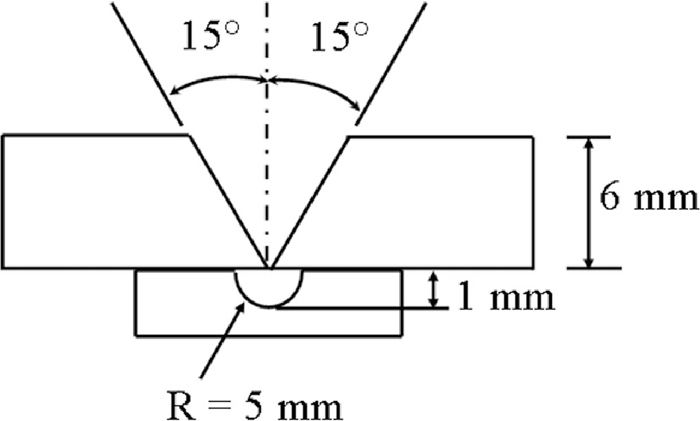
Schematic picture of original weld joint design.

Table 1. Chemical composition (in wt%) of base metal and filler wire.

Element	C	Mn	Si	S	P	Cr	Ni	Cu	V	Zr	Mo
Base metal	0.20	1.70	0.80	0.015	0.25	1.50	2	0.50	0.12	0.15	0.70
	max	max	max	max	max	max	max	max	max	max	max
Filler wire	0.08	1.20	0.68	0.012	0.012	–	–	0.02	–	–	–
	max	max	max	max	max			max

Table 2. Welding conditions considered in Figs. 7, 8 and 9.

Dataset No.	Welding current (A)	Welding voltage (V)	Welding speed (mm/s)	Heat Input (J/mm)	Wire feed rate (m/min)
1	290	29.50	11.6	735.5	8.5
2	252	24.64	8.3	743.8	7.5
3	310	30.33	11.6	809.7	9.5
4	310	30.33	10	939.3	8.5
5	315	30.25	8.3	1139.9	9.5

3. Theoretical Formulation

A three-dimensional transient heat transfer analysis is carried out to simulate gas metal arc welding (GMAW) process with the governing equation given as   

$$\frac{\partial }{\partial \mathrm{x}}\left(\mathrm{k}\frac{\partial \mathrm{T}}{\partial \mathrm{x}}\right)+\frac{\partial }{\partial \mathrm{y}}\left(\mathrm{k}\frac{\partial \mathrm{T}}{\partial y}\right)+\frac{\partial }{\partial \mathrm{y}}\left(\mathrm{k}\frac{\partial \mathrm{T}}{\partial z}\right)+\dot{\mathrm{Q}}=\rho {\mathrm{C}}_{\mathrm{P}}\frac{\partial \mathrm{T}}{\partial \mathrm{t}}$$(1)

where ρ, k and C_P refer respectively to density, thermal conductivity and specific heat of the workpiece material; t and T are time variables and temperature respectively. In Eq. (1), the term $\dot{Q}$ accounts for the arc heat input in terms of a volumetric heat source. The general boundary condition for typical heat condition analysis can be presented as   

$${\mathrm{k}}_{\mathrm{n}}\frac{\partial \mathrm{T}}{\partial \mathrm{n}}-\mathrm{q}+\mathrm{h}(\mathrm{T}-{\mathrm{T}}_0)+\sigma \epsilon ({\mathrm{T}}^4-{\mathrm{T}}_0^4)=0$$(2)

where n, k_n, h, ε, σ and T₀ refer to direction n normal to surface, thermal conductivity, surface heat transfer co-efficient, emissivity, Stefan-Boltzmann constant and the ambient temperature, respectively. The first term in Eq. (2) indicates a known temperature gradient normal to the boundary and regarded as positive inward. The second term q represents the applied surface heat flux and usually accounts for the arc heat input. In the present work, the arc heat energy is applied as a volumetric heat source ( $\dot{Q}$ ) as Eq. (3) rather than a surface heat flux (q) with the presumption that the surface heat flux would instantaneously establish a molten weld pool under the arc. The third and fourth term in Eq. (2) represents losses due to convection and radiation respectively. To avoid the non-linearity due to higher order terms associated with the radiation heat loss, a lumped heat transfer coefficient (h = 2.4×10^–3εT^1.61) is contemplated with the convective heat loss term.^15,17)

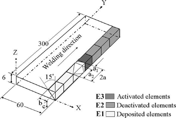
Figure 2 schematically presents the solution domain considered for the present analysis. A symmetric analysis is conducted with the plane of symmetry along the original weld groove center line. In Fig. 2, E1, E2 and E3 depict electrode materials that are already deposited, to be deposited and hence, deactivated and is being deposited and so, activated in the current time-step, respectively. Elements designated as E1 and E3 are assigned with the thermo-physical properties of work-piece material and the E2 set of elements are assigned with very small value of thermal conductivity to avoid their influence in the heat transfer analysis. In the beginning of each time-step, a new set of elements (E3) are activated at the liquidus temperature with the thermo-physical properties of the electrode material to consider the corresponding volume of electrode deposition. The movement of the volumetric heat source along the welding direction and the adoption of the depositions from the electrodes through E1 to E3 sets of elements are implemented in a finite element software through a user-defined subroutine.²¹⁾ The element edge length in the discretized geometry is varied between a minimum of 0.5 mm in the region below the welding arc to a maximum of 1.0 mm in the region away from the arc.

Fig. 2.

Schematic representation of double ellipsoidal volumetric heat source.

Figure 3 schematically shows two semi-ellipsoidal volumetric heat sources, as considered in the present work, with a smaller semi-ellipsoid in front of the arc center and a larger semi-ellipsoid at the rear are considered to account for the arc heat energy in the weld pool. The semi major axes, minor axes and depths of the front and the rear semi-ellipsoids are depicted as (a₁, b, c) and (a₂, b, c), respectively. The power density distribution in the front and the rear heat sources can be written as^5,7,14,17)   

$$\dot{\mathrm{Q}}=\frac{6\sqrt{3}{\mathrm{f}}_{\mathrm{i}}\mathrm{P}\eta }{\pi \sqrt{\pi }{\text{ a}}_{\text{i}}\text{ b c}}exp\left(-\frac{3{\mathrm{x}}^2}{{\mathrm{a}}_{\text{i}}^2}-\frac{3{\mathrm{y}}^2}{{\mathrm{b}}^2}-\frac{3{\mathrm{z}}^2}{{\mathrm{c}}^2}\right)$$(3)

Fig. 3.

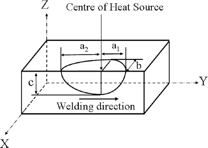
Schematic presentations of the two semi-ellipsoidal volumetric heat sources.¹⁵⁾

where the subscript i refers to 1 and 2 corresponding to the front and the rear heat sources, and η is the process efficiency. In Eq. (3), P is the arc power and estimated as P = αVI, where, α is the fraction of the available arc energy, I and V are the arc current and voltage, respectively. The values of α and η are considered as 0.75 and 0.80, respectively.^22,23,24,25) The values of f₁ and f₂ are considered as 0.6 and 1.4, respectively, as suggested in published literature.^{5,7,14,15,17)}

The values of a₁, a₂, b and c in Eq. (3) are obtained following an analytical approach. Assuming the heat source to be hemispherical, its geometric volume is given as   

$$\mathrm{\Omega }=\frac{\text{2}}{\text{3}}\pi {\text{a}}^{\text{3}}$$(4)

where a is the radius of the hemisphere. The geometric volume representing the arc heat source is considered to be equal to the volume of the molten workpiece plus the volume of molten electrode depositing in the V-groove and hence,   

$$\frac{\text{2}}{\text{3}}\pi {\text{a}}^{\text{3}}=\frac{\text{P}{\eta }_{\text{m}}{\text{t}}_{\text{S}}}{\rho {[\text{C}}_{\text{P}}{\text{(T}}_{\text{L}}-{\text{T}}_{\text{0}}\text{)}+\text{L}]}+\left[\left(\text{2}\times \frac{\text{1}}{\text{2}}{\text{(d}}^{\text{2}}\text{tan}\theta \right){\text{(vt}}_{\text{S}}\text{)}\right]$$(5)

where L is the latent heat, T_L and T₀ are the liquidus and ambient temperatures, respectively, d and θ refer to the depth and the half-groove angle of the V-groove, respectively, η_m is the melting efficiency and v is the welding speed. The energy transfer due to superheated weld droplets above liquidus temperature is neglected in Eq. (5). The melting efficiency (η_m) is considered as 0.50.^15,22,24,25) The first term on the right hand side of Eq. (5) refers to the volume of the molten workpiece under the welding arc for a given timestep, tS while the second term depicts the volume of V-groove to be filled by the electrode deposition during the same time-step. It is noteworthy that Eq. (5) allows an explicit determination of the radius, a, of the hemispherical heat source, which can be subsequently decomposed in the front and the rear semi-ellipsoids considering a₁ = f₁a and a₂ = f₂a, respectively, as indicated in Fig. 3. The depth, c, of both the front and the rear semi-ellipsoidal heat sources is the same and estimated as, $\text{c}=\sqrt{[{\text{a}}^{\text{2}}-{\text{(a}-{\text{a}}_{\text{1}})}^2]}$ . The semi-minor axis, b, of both the front and the rear semi-ellipsoidal heat sources will also be the same as, b =(2a³)/[(a₁ + a₂)c]. The determination of “a” indeed depends on the chosen timestep for a given welding speed and hence, in turn would influence the estimated power density as per Eq. (3). However, it is noteworthy that the net applied power is also solved for the same time-step thereby avoiding any unbalanced energy input. Secondly, the time-step values are so chosen such that the estimated dimension of the parameter “b”, which indirectly depicts the half-width of the volumetric heat source, should remain similar in magnitude to the typical presumed values of arc radius that is usually taken in the range of 1.5–3.0 times the electrode wire radius.²⁷⁾

Figure 4 schematically shows the weld reinforcement that is considered to be of parabolic profile with the reinforcement width, w_R, and height, h_R. Since the widths of the weld pool and the reinforcement usually remain nearly the same, w_R is presumed to be equal to be 2b. Hence, the reinforcement height, h_R, can be estimated by subtracting the volume of V-groove from the total estimated deposition from the electrode in a given time-step, t_S as   

$${\text{h}}_{\text{R}}=\left[\frac{\text{3}}{{\text{2W}}_{\text{R}}{\text{t}}_{\text{s}}\text{v}}\left(\frac{\pi {\phi }^2\text{e}\mathrm{\hspace{0.17em} }{\text{t}}_{\text{S}}}{\text{4}}-\left(\text{2}\times \frac{\text{1}}{\text{2}}{\text{(d}}^{\text{2}}\text{tan}\theta \right){\text{(vt}}_{\text{S}}\text{)}\right)\right]$$(6)

where φ is the diameter of the electrode wire and e is the wire feed rate. Equations (3) to (6) are used to estimate the dimensions of the volumetric heat sources corresponding to all the welding conditions (Table 2).

Fig. 4.

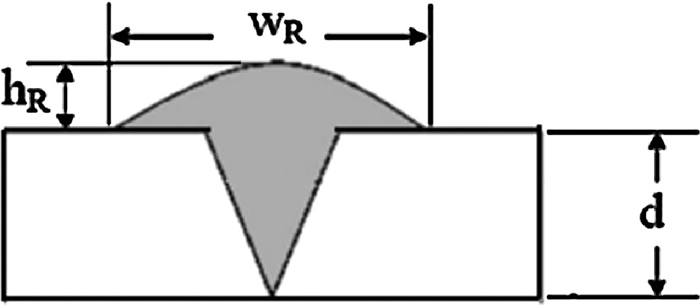
Schematic representation of the weld groove after the deposition.

4. Results and Discussion

Single-pass V-groove welds are performed on typical low carbon steel plates of 300 mm × 60 mm × 6 mm (thickness) with a groove angle (2θ) of 30° and zero root gap using the GMAW process. Table 3 depicts the temperature dependent material properties that are used for the model calculations. Figures 5(a) to 5(d) depicts a comparison of the computed weld pool profiles with the corresponding measured weld pool shapes for four different welding conditions. The computed weld pool profiles are represented in terms of the temperature isotherms with the zones heated above 1723 K and in between 1723 K and 996 K as the fusion zone and the HAZ, respectively. A comparison of Figs. 5(b) and 5(d) show decrease in the welding speed for a similar rate of heat input increases the reinforcement height. Smaller welding speed increases that volume of electrode deposition per unit length resulting in larger reinforcement height. A comparison of Figs. 5(a) to 5(c) depicts increase in bead dimensions with increase in the rate of heat input. The measured weld profiles depict typical finger shape penetration that indicates the influence of convective transport of heat in weld pool, which could not be accounted for in the heat conduction based model. The computed weld profiles in Figs. 5(a) to 5(d) depict typical elliptical shapes that have remained as an artifact of heat conduction based models of weld pool. Nevertheless, Figs. 5(a) to 5(d), in general, depict a fair agreement between the computed and the measured weld bead profiles.

Fig. 5.

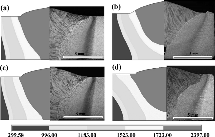
Comparison of experimentally measured and corresponding computed weld pool profile corresponding to the welding conditions (a) #4, (b) #2, (c) #3 and (d) #1 in Table 2. The value against the color map indicates temperature in K.

Table 3. Material properties of base metal and filler wire.

Density (ρ), kg mm–3	7.29×10–6
Thermal conductivity (k), Wm–1K–1	0.05 – (3.79×10–5×T)+ (1.65×10–8×T2)
Specific heat (C), J kg–1K–1	402.26 + (0.81×T) – (4.34×10–4×T2)
Solidus (TS) and Liquidus (TL) temperatures, K	1523, 1723
Latent heat (L), J kg–1	2.7 × 105

Figures 6(a) to 6(d) show a comparison between the computed and the corresponding experimentally measured thermal cycles at two different values of heat input (data sets #1 and #5 in Table 2). The longitudinal, transverse and depth locations of the thermocouples for the measured thermal cycle in Figs. 6(a) and 6(b) with regards to the reference frame of Fig. 2 are (51.1 mm, 172.7 mm, 6.0 mm) and (58.1 mm, 184.48 mm and 0 mm), respectively. Similarly the locations of the thermocouples in Figs. 6(c) and 6(d) are (54.1 mm, 157.9 mm, 6.0 mm) and (54.4 mm, 160.4 mm, 0 mm), respectively. The longitudinal distance is from the weld start point, the transverse distance is from the original weld interface and the depth is from the top surface. Figures 6(a) and 6(c) depict that as the heat input increases from 736 to 1140 J/mm, the measured cooling rate, ΔT_8/5 (from 1073 to 773 K), decreases from 28.8 to 13.71 K/s. The corresponding computed values of cooling rate, ΔT_8/5 are 20.75 and 9.90 K/s, respectively. Figures 6(b) and 6(d) show that the measured cooling rate, ΔT_8/5 (from 1073 to 773 K), decreases from 29.8 to 14.28 K/s and the corresponding computed values of cooling rate, ΔT_8/5 are 22.35 and 10.10 K/s, respectively. Increase in the rate of heat input results in greater weld pool volume and reduction in the cooling rate. A fair agreement between the computed and the corresponding measured values of peak temperature, thermal cycle and cooling rate is indicated in Figs. 6(a) to 6(d).

Fig. 6.

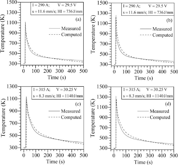
Comparison of experimentally measured and corresponding computed thermal cycles for two different welding conditions [(a) and (b) correspond to data set #1, and (c) and (d) correspond to data set #5 in Table 2].

Figures 7(a) to 7(d) depict the influences of several weld- ing conditions (shown in Table 2) on the measured and corresponding computed values of weld bead dimensions. The weld dimensions corresponding to data sets #2 and #5 depict that increase in the welding current from 252 to 315 A at constant welding speed increases the weld width from 7.83 to 10.52 mm, root width from zero to 4.10 mm, penetration from 5.2 to 6.0 mm and reinforcement height from 1.63 to 2.33 mm. The decrease in the welding speed from 11.6 to 10.0 mm/s at constant welding current (data sets #3 and #4) increases the root width from 2.20 to 2.44 mm, reinforcement height from 1.24 to 1.28 mm and weld width from 8.70 to 9.12 mm. An increase in welding current increases the overall rate of heat input resulting in greater weld width, penetration, reinforcement height and root width.

Fig. 7.

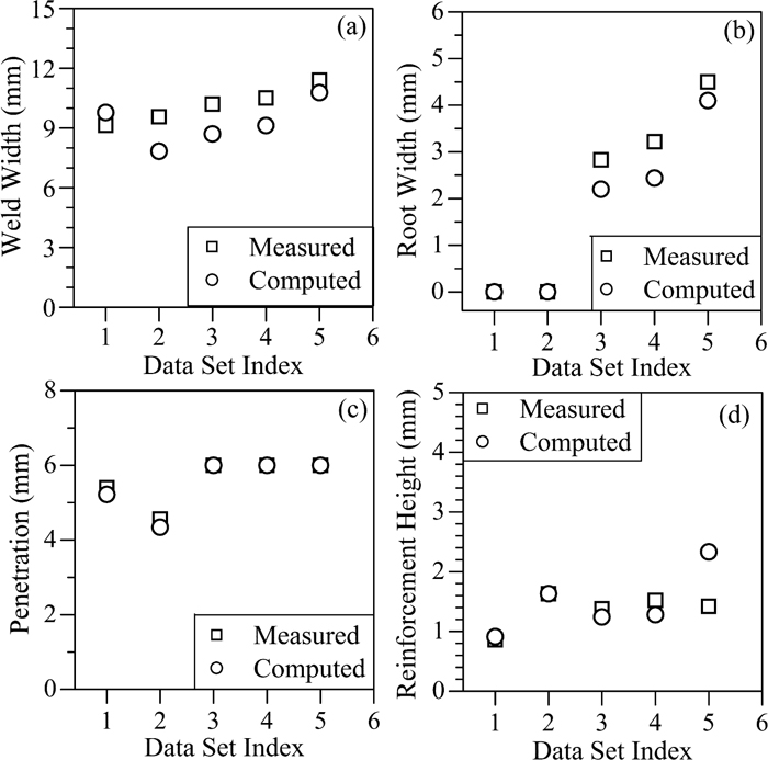
Comparison of the experimentally measured and corresponding computed weld dimensions for different welding conditions.

Figures 8(a) and 8(b) show the influence of several welding conditions (shown in Table 2) on the analytically estimated heat source dimensions and the corresponding numerically computed weld width and penetration. Increase in welding current from 252 to 315 A (data sets #2 and #5) enhances the estimated heat source width from 6.74 to 7.60 mm and the corresponding computed weld width from 7.83 to 10.78 mm [Fig. 8(a)]. Correspondingly, the estimated heat source depth increases from 2.83 to 3.19 mm and the numerically computed penetration increases from 4.34 to 6.0 mm [Fig. 8(b)]. Increase in welding current increases the rate of heat input and analytical estimation of heat source width and depth. Figures 8(a) and 8(b) also depict that the decrease in welding speed from 11.6 to 8.3 mm/s and increase in the welding current from 290 A to 315 A (data sets #1 and #5) increase the estimated heat source width and depth from 6.72 to 7.60 mm and 2.82 to 3.19 mm, respectively. The corresponding numerically computed values of weld width and penetration increase from 9.78 to 10.78 mm and 5.22 to 6.0 mm, respectively. Figures 8(a) and 8(b) demonstrate that the analytically estimated heat source dimensions [following Eqs. (5) and (6)] are able to account for the influence of welding conditions.

Fig. 8.

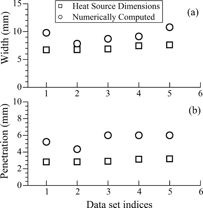
Comparison of the computed weld dimension and the estimated volumetric heat source dimensions for different welding conditions.

Realising the influence of welding process variables on the peak temperature and the cooling rates in the weld pool through experiments is difficult in GMAW process. The present work demonstrates that a heat transfer analysis considering a volumetric heat source to simulate welding arc can predict the bead dimensions, thermal cycle and cooling rate fairly in typical GMAW process. The volumetric heat source is analytically estimated as functions of welding condition and the initial joint geometry without any a priori assumption of final weld dimensions that would significantly improve the predictive capability of conduction based process simulation models in GMAW process.

5. Conclusions

A three-dimensional heat transfer model is presented for the analysis of gas metal arc welding process considering a volumetric heat source to account for the arc heat energy. The volumetric heat source is estimated analytically as function of welding conditions and original weld joint geometry, and without any a-priori assumption of the final weld bead dimensions. The electrode materials deposition is considered following activation and deactivation of the discrete elements in the original discretized solution domain. The final computed values of the weld bead geometry have indicated a fair agreement with the corresponding experimentally measured welds. A fair agreement is obtained between the numerically computed and the corresponding measured thermal cycles slightly away from the fusion zone. The overall approach and the computed results clearly indicate that heat conduction based model with analytically defined volumetric heat source as function of welding conditions and original joint geometry is able to provide a reliable estimation of weld bead profile and thermal cycle in gas metal arc welding.

Acknowledgement

The authors gratefully acknowledge the financial support provided by the DST, India (Grant no. INT/FRG/DAAD/P-212/2011) and DAAD, Germany (Grant No. 54368453) to carry out the present collaborative research work.

References

• 1)   S. A.  David and  T.  DebRoy: Science, 257 (1992), 497.
• 2)   T.  DebRoy and  S. A.  David: Rev. Mod. Phys., 67 (1995), 85.
• 3)   T.  Zacharia,  J. M.  Vitek,  J. A.  Goldak,  T.  DebRoy,  M.  Rappaz and  H. K. D. H.  Bhadeshia: Modell. Simul. Mater. Sci. Eng., 3 (1995), 265.
• 4)   A.  De and  T.  DebRoy: Sci. Tecnol. Weld. Join., 16 (2011), 4.
• 5)   P.  Tekriwal and  J.  Mazumder: Weld. J., 67 (1988), 150s.
• 6)   K. C.  Tsao and  C. S.  Wu: Weld. J., 67 (1988), 70s.
• 7)   E.  Pardo and  D. C.  Weckman: Metall. Trans. B, 20B (1989), 937.
• 8)   S.  Kumar and  S. C.  Bhaduri: Metall. Trans. B, 25B (1994), 435.
• 9)   J.  Jaidi and  P.  Dutta: Numerical Heat Trans. A, 40 (2001), 543.
• 10)   C. H.  Kim,  W.  Zhang and  T.  DebRoy: J. Appl. Phys., 94 (2003), 2667.
• 11)   H.  Nishiyama,  T.  Sawada,  H.  Takana,  M.  Tanaka and  M.  Ushio: ISIJ Int., 46 (2006), 705.
• 12)   A.  Kumar and  T.  DebRoy: Metall. Trans. A, 38A (2007), 506.
• 13)   J.  Hu and  H. L.  Tsai: Int. J. Heat Mass Trans., 50 (2007), 808, 833.
• 14)   A.  Mandal and  R. S.  Parmar: ISIJ Int., 47 (2007), 1485.
• 15)   D. V.  Kiran,  B.  Basu,  A. K.  Shah,  S.  Mishra and  A.  De: Sci. Technol. Weld. Join., 15 (2010), 111.
• 16)   A. R.  Lawrence and  P.  Michaleris: Sci. Technol. Weld. Join., 16 (2011), 215.
• 17)   D. V.  Kiran,  B.  Basu,  A. K.  Shah,  S.  Mishra and  A.  De: ISIJ Int., 51 (2011), 793.
• 18)   Z. H.  Rao,  S. M.  Liao and  H. L.  Tsai: Sci. Technol. Weld. Join., 16 (2011), 4.
• 19)   P. K.  Ghosh,  V. K.  Goyal,  H. K.  Dhiman and  M.  Kumar: Sci. Tecnol. Weld. Join., 11 (2011), 232.
• 20)   H. X.  Wang,  J. S.  Sun,  Y. H.  Wei and  Y. Y.  Zheng: Sci. Technol. Weld. Join., 10 (2011), 511.
• 21)  ANSYS 12 Theory Manual, SAS IP Inc., Pennsylvania, USA, (2009).
• 22)   J. F.  Lancaster: The Physics of Welding, Pergamon Press, New York, (1984), 204.
• 23)   N.  Pepe,  S.  Egerland,  P. A.  Colegrove,  D.  Yapp,  A.  Leonhartsberger and  A.  Scotti: Sci. Technol. Weld. Join., 16 (2011), 412.
• 24)   P. K.  Ghosh,  L.  Dorn,  K.  Devakumaran and  F.  Hofmann: ISIJ Int., 49 (2009), 251.
• 25)   P. K.  Ghosh,  L.  Dorn,  K.  Devakumaran and  F.  Hofmann: ISIJ Int., 49 (2009), 261.
• 26)   S.  Bag and  A.  De: Metall. Trans. A, 39A (2008), 2698.