Validation and Calibration Approach for Discrete Element Simulation of Burden Charging in Pre-reduction Shaft Furnace of COREX Process

Abstract

Discrete element method (DEM) has been an increasingly used tool to get better understanding of charging process and flow behaviors of granular materials in metallurgical reactors. However, validation and precision of DEM must be verified and calibrated. In this paper, a calibration approach is proposed for the sphere equivalence of irregular particles in DEM simulation of charging process. In this approach, the non-sphere behavior of irregular particles is characterized by a pair of apparent sliding and rolling resistance coefficients obtained by quantitative comparison of the angle of repose and discharging time of hopper based on laboratory measurement of physical benchmarking experiments. The calibration approach is applied in the DEM simulation of the charging process of a shaft furnace in COREX 3000. Validation of simulation results for flow trajectory and stream width after leaving chute and burden distribution and profile is investigated through comparison of DEM and experiments. The results show that, with such a calibration approach, DEM can be easily used to simulate solid flow of irregular particles.

1. Introduction

COREX process consists of two reactors, the pre-reduction shaft and the melter-gasifier and the pre-reduction shaft is placed above the melter-gasifier.^1,2,3,4) Mixture of iron bearing burden and some amount of coke is continuously charged into the pre-reduction shaft by the Gimbal distribution system.⁵⁾ The reduction gas is injected through the bustle located in the lower-middle of the shaft and rises in the counter current direction to the top of the shaft. The distribution of reducing gas affects the temperature profile, gas utilization rate, metallization degree and other economic indices. And the gas flow distribution mainly depends on the burden charging behaviors. Furthermore, the burden distribution behaviors directly dominate gas flow distribution, heat transfer and reduction reaction rate, thus the total furnace performance.

The essential of burden distribution is a granular material charging process involving of a large number of solid particles moving through a hopper, a downstream tube, a rotating chute, and at last free falling on burden surface in a shaft.^6,7,8) Although the operating principle in COREX pre-reduction shaft and in blast furnace differs, the knowledge of iron-making blast furnace built would be the foundation for understanding of COREX. A great effort has been paid toward enhancing the comprehending of charging behaviors for blast furnace.^{9,10,11,12,13,14,15,16,17)} Radhakrishnan et al. had developed a mathematical model for predicting the particle trajectories and stockline geometry based on constructing equations by consideration of the flow of different types of solid particles like iron ore, sinter and coke through the bin and rotating chute.⁹⁾ Kajiwara et al. firstly reported a 2-D discrete element model to simulate the formation of burden distribution at blast furnace top and successfully analyzed slope angle of stock line influence on the burden deposit behavior and size segregation phenomenon.¹⁰⁾ Matsuzaki et al. carried out a study on segregation behaviors of charging process affected by particle density, shape and size with the use of laboratorial model apparatus and a 2-D discrete element model.¹¹⁾ Inada et al. presented a mathematical model for the estimation of the radial particle size distribution and successfully applied to the test operation of large bell stroke control.¹²⁾ More recently, Mio et al. established a particle flow simulator¹³⁾ for a blast furnace charging process using the discrete element method and discussed the particle density distribution,¹⁴⁾ particle size segregation,¹⁵⁾ effect of chute angle¹⁶⁾ and traveling behavior of nut coke¹⁷⁾ in bell-type charging process of blast furnace.

Discrete element method has been increasingly used to get better understanding of this complicated particulate charging process.^18,19,20) However, validation and precision of discrete element method must be calibrated when developing a 3-D numerical simulation model of burden distribution for the pre-reduction shaft furnace of COREX 3000.^21,22) In this paper, a validation and calibration approach is proposed to determine the input parameters for DEM through quantitative comparison of the angle of repose and discharging time of hopper based on laboratory measurement of physical calibration experiments. Then validation of flow trajectory and stream width after leaving chute and burden distribution and profile is investigated through comparison of DEM and experiments. The proposed benchmarking test method may provide a possible means to guarantee the sphere particles to meet the equivalent charging behaviors of irregular particles through determining a pair of apparent sliding and rolling resistance coefficients in DEM.

2. Discrete Element Model

The elementary units of granular materials are mesoscopic particles, and then every single particle undergoing translational and rotational motions is tracked through force-displacement relationship^23,24) as illustrated in Fig. 1. The macroscopic and microscopic information can be captured by collection of particle information. The governing equations for the translational and rotational motions of particle i with radius R_i, mass m_i and moment of inertia I_i can be written respectively as   

$$m_i\frac{d^2{\mathbf{x}}_i}{d{t}^2}+\eta \frac{d{\mathbf{x}}_i}{dt}+K{\mathbf{x}}_i+{\mathbf{F}}_{\text{v},i}+{\mathbf{F}}_{\text{s},i}=\text{0}$$(1)

  

$$I_i\frac{d^2{\theta }_i}{d{t}^2}+{\eta }_{\text{r}}\frac{d{\theta }_i}{dt}+K_{\text{r}}{\theta }_i=0$$(2)

where x_i, θ_i, η, K are, respectively, the translational displacement, the rotational angle, the damping and stiffness coefficients of particle i, and subscript r denotes the rolling parameters. The forces involved are: the body force, F_v,i, including gravitational force, m_ig, the surface force, F_s,i, such as fluid-particle interface force. The translational motion is decomposed into two components in the normal and tangential directions. Focusing on the interactions between particles and ignoring the interaction with gas phase, the above equations can be simplified as follows.   

$$m_i\frac{d{\mathbf{v}}_i}{dt}=\sum _{j=1}^{k_i}({\mathbf{F}}_{\text{n},ij}+{\mathbf{F}}_{\text{t},ij})+m_i\mathbf{g}$$(3)

  

$$I_i\frac{d{\omega }_i}{dt}=\sum _{j=1}^{k_i}({\mathbf{M}}_{\text{t},ij}^{}+{\mathbf{M}}_{\text{r},ij}^{})$$(4)

where v_i, ω_i are, respectively, the translational and angular velocities of particle i; F_c,i= F_n,ij+F_t,ij is the inter-particle contact force between particles i and j; F_n,ij and F_t,ij, are, respectively, the normal and tangential components of contact force, which includes the elastic force F_e,ij and viscous damping force F_d,ij. The torque acting on particle i by particle j includes two components: the rolling resistance torque and torque arising from tangential force. For a particle i undergoing multiple interactions, the individual interaction forces and torques are summed up for the other k_i particles interacting with particle i. The rolling resistance^24,25,26,27) plays an important role in the formation of burden profile. For effect of particle shape on charging process, Jiang’s model²⁴⁾ is used in this work. The inter-particle forces are calculated based on non-linear contact models^28,29,30) which are listed in Table 1. The Coulomb-type friction law is taken into account by truncating the tangential overlap of the contact in order to meet |F_t,ij| <=μ_s|F_n,ij| with μ_s being the sliding friction coefficient.

Fig. 1.

The contact model adapted by this paper proposed by Jiang,²⁴⁾ which consist of normal, tangential and rolling contact components: a normal contact model for normal force, a tangential contact model for shear force and a rolling contact model for rolling.

Table 1. Components of forces and torque acting on particle i.

Forces and torques	Symbol	Equations
Normal elastic contact force	Fen,ij	–Knδn	$K_{\text{n}}=\frac{4}{3}{E}^{*}\sqrt{R^{*}\left|{\delta }_{\text{n}}\right|}$
Normal damping force	Fdn,ij	–ηnVn,ij	${\eta }_n=-\text{2}\sqrt{\frac{\text{5}}{\text{4}}}\beta \sqrt{m^{*}{K}_{\text{n}}}$
Tangential elastic contact force	Fet,ij	–Ktδt	$K_{\text{t}}={\text{8G}}^{*}\sqrt{R^{*}\left|{\delta }_{\text{n}}\right|}$
Tangential damping force	Fdt,ij	–ηtVt,ij	${\eta }_{\text{t}}=-\text{2}\sqrt{\frac{\text{5}}{6}}\beta \sqrt{m^{*}{K}_{\text{t}}}$
Torque arising from tangential force	Mt,ij	R*n × (Fet,ij + Fdt,ij)
Rolling resistance torque	Mr,ij	–Krθr θr<=θ0	$K_{\text{r}}=\frac{K_n{B}^2}{12}$
		M0 θr>θ0	${\mathbf{M}}_0=\frac{\mathbf{n}\times ({\mathbf{F}}_{en}+{\mathbf{F}}_{dn})B^2}{6}$

Where, $\frac{1}{E^{*}}=\frac{{(1-{\nu }_i)}^2}{E_i}+\frac{{(1-{\nu }_j)}^2}{E_j}$ , $\frac{1}{G^{*}}=\frac{2(2+{\nu }_i)(1-{\nu }_i)}{E_i}+\frac{2(2+{\nu }_j)(1-{\nu }_j)}{E_j}$ , $\frac{1}{R^{*}}=\frac{1}{R_i}+\frac{1}{R_j}$ , $\frac{1}{m^{*}}=\frac{1}{m_i}+\frac{1}{m_j}$ , $\beta \frac{ln(\mathrm{e})}{\sqrt{{ln}^2(\mathrm{e})+{\pi }^2}}$ , ${\delta }_{\text{n}}=\left[\left(R_i+R_j\right)-\left|{\mathbf{x}}_i-{\mathbf{x}}_j\right|\right]\mathbf{n}$ , V_n,ij =(V_ij·n)·n, V_t,ij =(V_ij×n)×n, V_ij =V_j–V_i+ω_j×R_j–ω_i×R_i, $\mathbf{n}=\frac{{\mathbf{x}}_j-{\mathbf{x}}_i}{\left|{\mathbf{x}}_j-{\mathbf{x}}_i\right|}$ ; E is Young’s Modulus; ν is Poisson ratio; B is a contact width defined as B=φR^*, where the quantity φ is a dimensionless material and geometrical parameter which will generally be related to grain shape; δ_t is the vector of the accumulated tangential displacement between particles i and j; subscript en, et, dn and dt are, respectively, the normal and tangential directions of the elastic and damping forces. Young modulus and Poisson ratio of yellow rice and soybean are E_rice=7.5 MPa, ν_rice=0.35, E_soybean=2.5 MPa, ν_soybean=0.25, respectively.

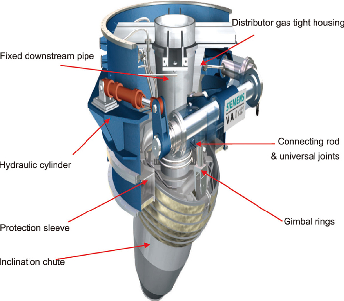
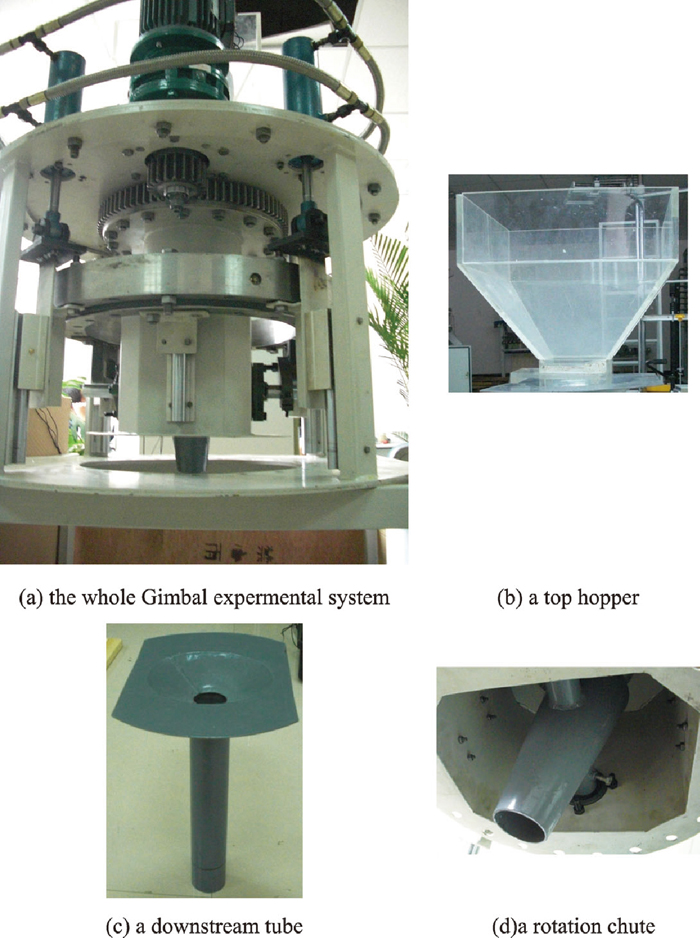
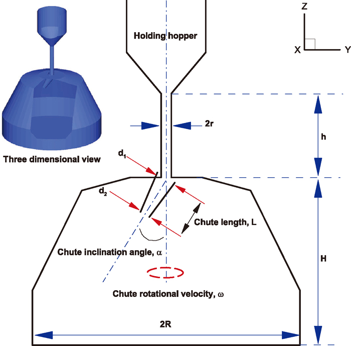
The simulation object is a Gimbal top charging system, which located on the top centre of COREX pre-reduced shaft furnace. The real distributor used in a commercial plant⁵⁾ is shown in Fig. 2 and its corresponding simplified physical experimental device is given in Fig. 3, Geometry schemes of DEM simulations and experiments adopted by this work are illustrated in Fig. 4. The geometry parameters in the simulation are listed in Table 2. The particles with mono-sized diameter for soybean of 7.1 mm and yellow rice of 3.5 mm are used, respectively.

Fig. 2.

Gimbal top charging system.⁵⁾

Fig. 3.

Experimental device for Gimbal top charging system, with a top hopper, a center downstream tube and truncated cone rotation chute from bottom-side view.

Fig. 4.

Geometry of charging system and distribution chute of the COREX shaft used in experiments and discrete element simulations.

Table 2. Geometry parameters used in experiments and simulations.

Fixed center fall pipe radius, r	30 mm
Fixed center fall pipe height, h	500 mm
Diameter of chute inlet, d1	60 mm
Diameter of chute outlet, d2	30 mm
Chute length, L	250 mm
Chute inclination angle, α	0–31.5°
Shaft throat radius, R	1600 mm
Stock line height, H	900 mm

3. Results and Discussion

3.1. Calibration Approach for Frictional Coefficients

The Angle of Repose (AoR) is defined between the slope of the pile and the horizontal ground, which has a significant effect on burden profile of charging process. So AoR can be used as a quantitative calibration tool. It must be guaranteed that the material property parameters used in simulation can give the same AoR as actual burden-iron ore or coke material. Thus a series of numerical simulation and experiments were conducted to calibrate the material property parameters including sliding frictional coefficient and rolling frictional coefficient.

For the AoR measurements, the so-called “free-base piling” experiment³¹⁾ is adopted. Firstly, the testing particles are fully filled in a scale-down hopper, which is hung up a certain distance from the stockline. Sample particles are then discharged from the hopper and form a conical pile on the ground. The slope of the pile and the horizontal ground is defined as the AoR of the testing sample. Measurements are conducted along with cross direction, and then the AoR is calculated through averaging four-direction measured data. The same experiment process is repeated three times.

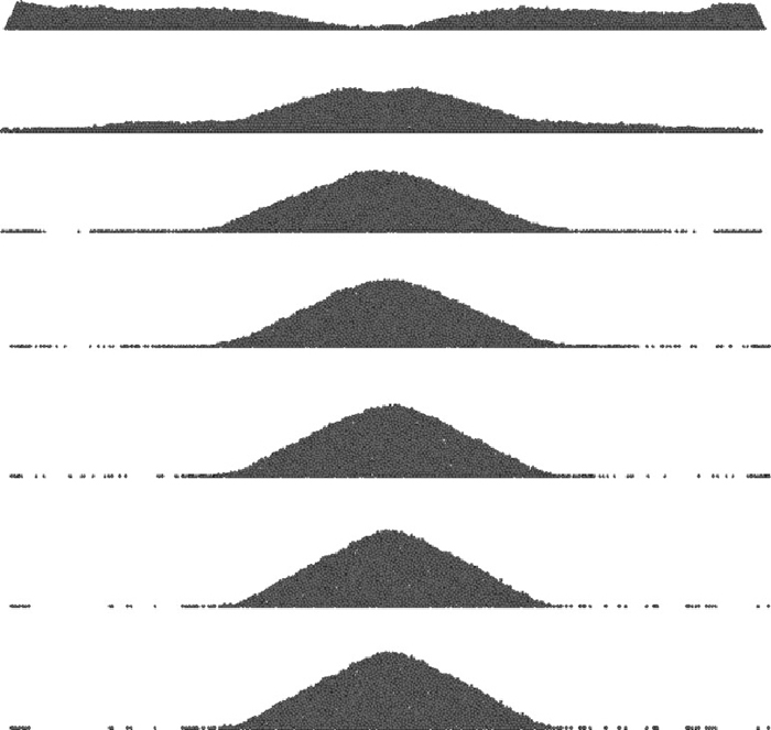
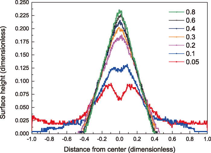
Figure 5 shows the profiles of burden pile for soybean from DEM simulation with different sliding frictional coefficients when rolling resistance is set as zero. The profiles of burden piles are clearly different. The pile surface slope increases greatly as the sliding frictional coefficient is increased. Especially for small sliding frictional coefficients, not only granular pile can not be formed, but even a cavity is created. Taking Fig. 6 at 0.1 of rolling resistance coefficient as an example, the quantitative comparison of surface profiles for soybean with the different the sliding frictional coefficients is shown in Fig. 6. Its’ x-axis, which has been normalized from –1 to 1 for dimensionless analysis, denotes the distance from the pile center, and the y-axis is the height of the pile, which has also been normalized correspondingly to x-axis. With the increase of sliding friction coefficient, the surface slope of pile becomes steeper, but the change rate of AoR slows down significantly.

Fig. 5.

Burden profiles at various sliding frictional coefficients without rolling resistance, with μ_s at 0.05, 0.1, 0.2, 0.3, 0.4, 0.6 and 0.8, from top to bottom, respectively, and particle diameter of 7.1 mm.

Fig. 6.

Comparison of surface profiles for different the sliding frictional coefficients with rolling resistance coefficient φ = 0.1.

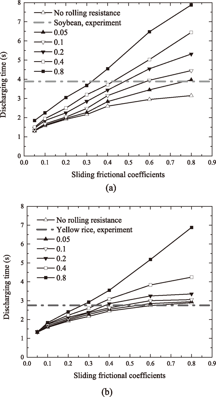
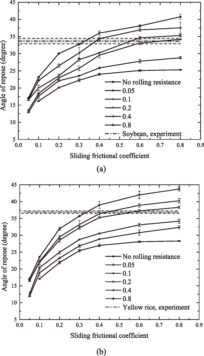
To clarify the role of rolling resistance, Figs. 7(a) and 7(b) shows the simulation results of piles with different rolling resistances in terms of various AoRs for soybean and yellow rice, respectively. It can be seen that AoR depends significantly on rolling resistance, and the AoR with low rolling resistance is remarkably smaller than that with high rolling resistance. Moreover, while the rolling resistance is set as zero, particles collection will behave with high mobility, resulting in a flat pile. The rolling resistance difference arises from the difference in particle shape, and will result in different energy dissipating rate. The error bars in Fig. 7 comes from the measurements at different directions. The measured average values of experimental results are presented in Figs. 7(a) and 7(b) by the horizontal dash-dot line for soybean (called A line) and yellow rice, respectively. The shaded areas illustrate the deviation of measurements to averaged value, which comes from the measurements at different directions. There are two series of experimental measurements hence two series of experimental results. The points of intersections between curves and horizontal lines show that the best agreement with these two experimental values can lead to multiple combinations between sliding and rolling coefficients. So another experimental indicator is needed to determine the unique solution. For this reason, when the AoR experiments were conducted, the discharging time was also recorded simultaneously by digital stopwatch. Here the average discharge time (ADT) is used. Figures 8(a) and 8(b) shows the effect of sliding frictional coefficient on ADT from DEM simulation with different rolling resistance coefficients, and experimental results of ADT for soybean (called B line) and yellow rice are also given in figure. The optimum values of the pairs of sliding and rolling frictional coefficients of soybean for example, must simultaneously satisfy Figs. 7(a) and 8(a). To determine the optimum values, Set A and Set B are built by collecting all the pairs of sliding and rolling frictional coefficients along A line in Fig. 7(a) and B line Fig. 8(a), respectively. Note that these two sets can be enriched by linear interpolation in case of need. Then the matching pair, i.e. the pair of unique values appears in these to sets is selected as the sliding and rolling frictional coefficients for soybean. With the same procedure, the sliding and rolling frictional coefficients for yellow rice can also be obtained. In this way, the pairs (μ_s, μ_r ) of (0.61, 0.12) and (0.32, 0.43) are obtained for soybean and yellow rice, respectively.

Fig. 7.

Effect of sliding friction coefficient on angle of repose for various rolling resistance coefficients. (a) soybean and (b) yellow rice.

Fig. 8.

Effect of sliding frictional coefficient on discharging time for different rolling resistance coefficients. (a) soybean and (b) yellow rice.

3.2. Validation of Particles Flow Trajectories and Width

Using the determined parameters, discrete element simulations are then conducted to investigate particles flow after leaving the chute for charging process. Figure 9 shows a simulation example in visual comparison with experiment. Conditions of simulation and experiment are α=15°, ω=0.12 cycles/s, d_soybean=7.1 mm, d_rice=3.5 mm, charging mass=52.15 kg, soybean to yellow rice mass ratio = 2:8. As shown in Fig. 9, the burden flow characteristics, such as the trajectory and width of burden flow, can be reproduced through calibrating DEM simulation. Furthermore, it is found in the simulation that there are always some small particles flying out from the centre of burden flow. Such a feature is consistent with the observed phenomena in the physical benchmarking experiments. This is due to the strong particle-particle interactions. The velocity direction of small particle is easy to change after collision with big particle, leading to splash of small particles. So, in burden flow simulation of charging process, the force between particles cannot be ignored.

Fig. 9.

Example of comparison for flow characteristics of burden in charging process. (a) experiment, (b) DEM simulation.

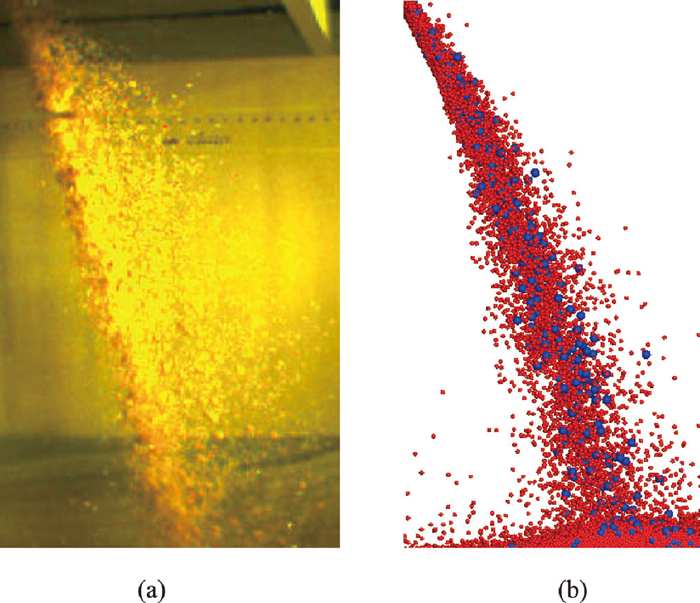
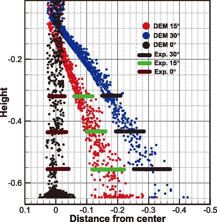
Figure 10 further shows a quantitative comparison of flow trajectories and stream width between simulated and experimental results for soybean with different chute inclination angle. Three different chute inclination angles of 0°, 15° and 30° from DEM simulation are selected for comparison with experimental results. Both of DEM and experiments show that the stream has a certain width after leaving the rotating chute, and three types of trajectories can be determined: upper surface flow, flow of centroid and lower surface flow. With the increase of chute inclination angle, such flow characteristics become more pronounced. By and large, the simulation results match the experiments, indicating that DEM model can produce consistent trajectories and flow width feature with physical experiments, but there is still some minor difference, as shown in Fig. 10, where the simulated particles flow width deviate slightly from experiments when chute angle is 30°.

Fig. 10.

Comparison of trajectories and flow width for different chute inclination angles.

3.3. Validation of Burden Profile

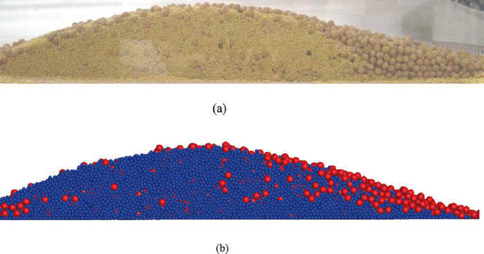
For charging process, the most concerned results are the burden profile, composition radial distribution, segregation, as well as porosity distribution. A laboratory scale experiments and simulations of burden charging process of the Gimbal distributor of pre-reduction shaft were conducted for determining burden profile. Figure 11 shows the visual comparison for burden profile and segregation behaviours for chute inclination angle of 15 degree with 0.12 cycles/s of rotational speed. Figure 11 is a cross section of burden profile, and when a batch of charging test was finished, the stockpile will be formed, a very thin transparent glass plate is slowly inserted into the heap along a conical pile, and then the particles were all removed in a side of the glass plate, and the other side can be captured by a camera as shown in Fig. 11. It can be noticed in the experiments, as well as in DEM simulations, that particle rolling on the burden surface is quite obvious in the charging process. Bigger particles gather in the bottom of burden slope, leading to the segregation of different size particles.

Fig. 11.

Example of burden profile and segregation behaviors for mixed charging process at chute inclination angle of 15°. (a) experiment, (b) simulation. Where small particles are yellow rice and large one are soybeans.

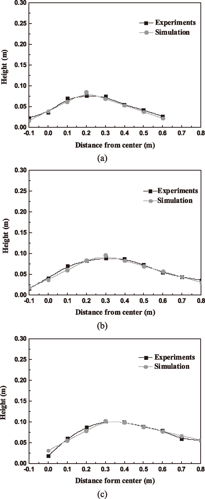
Further quantitative comparisons between the results of the experiments and DEM simulations are provided in Fig. 12, which show a side view of the burden bed and the surface profiles. In Fig. 12, the experimental data represent the average values of four measurement sets along different radial directions and the average values of corresponding radius circumference are extracted from DEM simulations. One can see clearly that the effect of chute angle on burden profile. It can also be observed that the peak of burden profile of charged particles moves toward the side-wall of furnace with increasing the chute angle. Comparing the calculated burden profile with the experimental one, a quite good consistency is seen, although the peak value of burden profile of DEM simulation is always a little higher than the one in the experiment. Overall, it can be concluded that the simulations and experiments show good agreement.

Fig. 12.

Comparison of burden profile between experiment and simulation at different chute inclination angles. (a) 10°, (b) 15° and (c) 20°.

3.4. Simulator of Charging Process

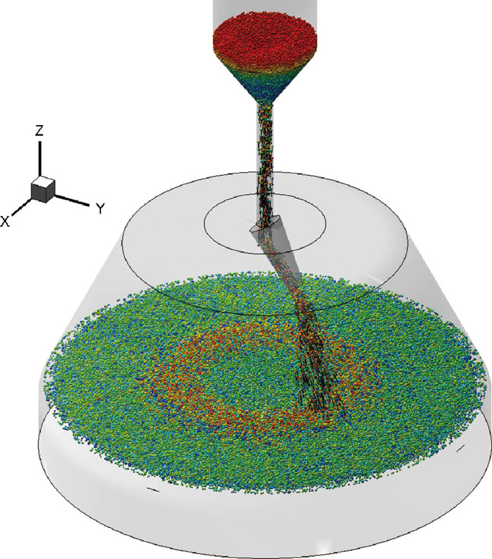
DEM simulation as particle-scale method has demonstrated a more advantageous potential than traditional physical experiments, i.e. more microscopic-scale information can be obtained. Based on the discrete element simulation, a simulator of burden charging in pre-reduction shaft furnace of COREX process is developed and calibrated and validated. A snapshot of charging process using this simulator is shown in Fig. 13. As the initial condition, there are altogether 100,000 particles randomly generated in the hopper with the soybean to yellow rice mass ratio of 2:8 and 100,000 particles in the shaft. After opening the hopper outlet, the particles flow down through the fixed center pipe and the rotating tilting chute. The chute, with an inclination angle of 15 degree, rotates at 0.12 cycles/s. In the end the burden pile is formed.

Fig. 13.

A snapshot of charging process of COREX 3000 pre-reduction shaft (color by particle id number).

4. Summary

A calibration approach is proposed for the sphere equivalence of irregular particles in DEM simulation of charging process. Angle of repose and discharging time are selected as benchmarking calibration rule for justifying the sliding and rolling frictional coefficients in this approach. The non-sphere behavior of irregular particles is characterized by a pair of sliding and rolling resistance coefficients obtained by benchmarking experimental data. The calibration approach is applied in the DEM simulation of the charging process of a shaft furnace in COREX 3000. Validation of calibrated DEM model for particles flow width and burden profile for different chute inclination angles has been verified through visual and quantitative comparison between DEM simulations and experiments. The results show that, with such a calibration approach, DEM can be easily used to simulate solid flow of irregular particles and shows consistence with experiment results.

Acknowledgement

The authors are grateful to the National Natural Science Foundation of China (grant No. 51104037 and No. 51174053) for the financial support of this work.

Reference

• 1)   S.  Wu,  J.  Xu,  S.  Yang,  Q.  Zhou and  L.  Zhang: ISIJ Int., 50 (2010), 1332.
• 2)   Y.  Qu,  Z.  Zou and  Y.  Xiao: ISIJ Int., 52 (2012), 2186.
• 3)   S.  Lee,  M.  Shin,  S.  Joo and  J.  Yoon: ISIJ Int., 40 (2000), 1073.
• 4)   S.  Lee,  M.  Shin,  S.  Joo and  J.  Yoon: ISIJ Int., 39 (1999), 319.
• 5)   M.  Riddle and  P.  Whitfield: Ironmaking Steelmaking, 34 (2007), 221.
• 6)   H.  Zhao,  M.  Zhu,  P.  Du,  S.  Taguchi and  H.  Wei: ISIJ Int., 52 (2012), 2177.
• 7)   J.  Park,  U.  Baek,  K.  Jang,  H.  Oh and  J.  Han: ISIJ Int., 51 (2011), 1617.
• 8)   S.  Nag,  M.  Guha,  S.  Kundu,  S. K.  Sinha and  U.  Singh: ISIJ Int., 48 (2008), 1316.
• 9)   V. R.  Radhakrishnan and  K. M.  Ram: J. Process Control, 11 (2001), 565.
• 10)   Y.  Kajiwara,  T.  Inada and  T.  Tanaka: Tetsu-to-Hagané, 75 (1989), 235.
• 11)   S.  Matsuzaki and  Y.  Taguchi: Tetsu-to-Hagané, 88 (2002), 823.
• 12)   T.  Inada,  Y.  Kajiwara and  T.  Tanaka: ISIJ Int., 29 (1989), 761.
• 13)   H.  Mio,  M.  Kadowaki,  S.  Matsuzaki and  K.  Kunitomo: Miner. Eng., 33 (2012), 27.
• 14)   M.  Akashi,  H.  Mio,  A.  Shimosaka,  Y.  Shirakawa,  J.  Hidaka and  S.  Nomura: ISIJ Int., 48 (2008), 1500.
• 15)   H.  Mio,  S.  Komatsuki,  M.  Akashi,  A.  Shimosaka,  Y.  Shirakawa,  J.  Hidaka,  M.  Kadowaki,  S.  Matsuzaki and  K.  Kunitomo: ISIJ Int., 48 (2008), 1696.
• 16)   H.  Mio,  S.  Komatsuki,  M.  Akashi,  A.  Shimosaka,  Y.  Shirakawa,  J.  Hidaka,  M.  Kadowaki,  S.  Matsuzaki and  K.  Kunitomo: ISIJ Int., 48 (2009), 479.
• 17)   H.  Mio,  S.  Komatsuki,  M.  Akashi,  A.  Shimosaka,  Y.  Shirakawa,  J.  Hidaka,  M.  Kadowaki,  H.  Yokoyama,  S.  Matsuzaki and  K.  Kunitomo: ISIJ Int., 50 (2010), 1000.
• 18)   Y.  Yu and  H.  Saxén: Adv. Powder Technol., 22 (2011), 324.
• 19)   H. P.  Zhu,  Z. Y.  Zhou,  R. Y.  Yang and  A. B  Yu: Chem. Eng. Sci., 62 (2007), 3378.
• 20)   H. P.  Zhu,  Z. Y.  Zhou,  R. Y.  Yang and  A. B  Yu: Chem. Eng. Sci., 63 (2008), 5728.
• 21)   R. B.  Smith and  M. J.  Corbett: Ironmaking Steelmaking, 14 (1987), 49.
• 22)   K. P.  Prachethan,  L. M.  Garg and  S. S.  Gupta: Ironmaking Steelmaking, 33 (2006), 29.
• 23)   P. A.  Cundall and  O. D. L.  Strack: Géotechnique, 29 (1979), 47.
• 24)   M. J.  Jiang,  H. S.  Yu and  D.  Harris: Comput. Geotechnics, 32 (2005), 340.
• 25)   J.  Ai,  J.-F.  Chen,  J. M.  Rotter and  J. Y.  Ooi: Powder Technol., 206 (2011), 269.
• 26)   M.  Oda and  K.  Iwashita: Int. J. Eng. Sci., 38 (2000), 1713.
• 27)   K.  Iwashita and  M.  Oda: ASCE J. Eng. Mech., 124 (1998), 285.
• 28)   A.  Di Renzo and  F. P.  Di Maio: Chem. Eng. Sci., 60 (2005), 1303.
• 29)   A.  Di Renzo and  F. P.  Di Maio: Chem. Eng. Sci., 59 (2004), 525.
• 30)   N. V.  Brilliantov,  F.  Spahn,  J.-M.  Hertzsch and  T.  Poeschel: Phys. Rev. E, 53 (1996), 5382.
• 31)   W.  Wang,  J.  Zhang,  S.  Yang,  H.  Zhang,  H.  Yang and  G.  Yue: Particuology, 5 (2010), 482.