Flatness Intelligent Control Based on T-S Cloud Inference Neural Network

Abstract

The accuracy of traditional flatness control methods are limited and it is difficult to establish a precise mathematical model of the rolling mill. In addition, the flatness control system is complex and multivariate. General model approaches can not satisfy the high precision demand of rolling process. In this paper, T-S cloud inference neural network and its stability are proposed. It is constructed by cloud model and T-S fuzzy neural network. The stability of T-S cloud inference neural network is analyzed by Lyapunov method in details. Based on the new network, flatness recognition model and flatness predictive model are established. And they are applied for 900HC reversible cold rolling mill. The flatness control system is designed and a simple controller is developed. Initial parameters of the controller are firstly determined through offline training based on measured data, and then they are optimized online automatically. Genetic Algorithm (GA) is used as the optimizing method which is compared with particle swarm optimization (PSO). The simulation results demonstrate that the flatness control system is effective and has a better precision and robustness.

1. Introduction

Flatness control is a key technology of the cold rolling strip steel production. It is also a hot research topic in the current international. With the rapid development of economy, the precision of flatness is becoming more and more accurate.¹⁾ Strip steel is the main products of rolled steel, and it is widely used in buildings, bridges, ship buildings and cars. Flatness is a significant quality indicator of strip steel. The purpose of flatness research is to solve the accuracy of flatness control. However, the accuracy of traditional flatness control methods is limited, and it is difficult to establish a precise mathematical model of the rolling mill. The rolling process is multivariate, strong-coupling, nonlinear, and time-varying. So, the flatness theory needs to be studied deeply and extensively. Building an accurate, stable, fast model of flatness control has become a development direction of flatness control technology.²⁾

Artificial intelligence (AI) technique is an efficient alternative tool for complex and nonlinear system modeling in many disciplines.^3,4,5,6,7) Specialists and scholars have applied AI to the area of rolling and many new theories and algorithms have been widely used. The development of intelligent control provides new thinking and ways for flatness control technology. Zhang⁸⁾ utilized internal model control method based on feed-forward neural network to train the neural network recognizer and internal model controller offline. And improved BP algorithm is used for adjusting the weights online. Simulation results showed that the hydraulic bending roll system possessed rapid response and strong robustness and the control effect is ideal. Wang and Li⁹⁾ combined PSO with GA algorithm and the mixed algorithm was applied for the adaptive PID control of hydraulic bending system. A simulation model was built and a better control performance was got. Based on conventional PID control algorithm, Shan et al.¹⁰⁾ built an optimized nonlinear combined control rule of P, I, and D by the self-learning ability of neural network and the “conception” abstraction ability of fuzzy control. Simulation results of the model indicated that flatness target value was tracked well with rapid response, small overshot and strong robust. In order to resolve the problem of low precision, slow speed and bad anti-interference ability in conventional PID flatness control, Jia et al.¹¹⁾ proposed the strategy of single-nerve -cell adaptive PID flatness control based on BP neural network prediction model. Simulation results indicated that the control algorithm can track the target set value of flatness, increase the control precision of the system and accelerate the response speed of the system with strong anti- interference ability. Fan¹²⁾ designed a fuzzy controller. Through the membership function and quantification factors and scaling factors, the controller was adjusted by the fuzzy control rule table. It has certain adaptive ability.

Based on probability theory and fuzzy mathematics, a new model, called cloud model, is proposed by academician Deyi Li. This model not only reflects the uncertainty of natural language concepts, but also presents the correlation between randomness and fuzziness. It is an uncertainty transformation model between qualitative concept and its quantitative representation which are described by linguistic value. Zhang et al.¹³⁾ proposed a method of implementing intelligent control of inverted pendulum by the use of cloud models. Its control strategy needs no mathematical models of plant but human experience, sensation and logic decision. The experiment results demonstrated that the method had stronger robustness against the variation of states and parameters of plants, and that it had better practicing value and widely prospect. Liu and Li¹⁴⁾ designed a fuzzy system based on the combination of cloud model theory and neural network. And the system resolved the difficulties of the definition of the subjection function and knowledge regularity in the practical application of fuzzy system. Xu and Fan¹⁵⁾ proposed an approach of cloud neural network which was used for fault detection and diagnosis of the space propulsion system.

T-S fuzzy neural network was firstly proposed by Takagi and Sugeno. This model utilizes local linear equation to replace constant which is usually in general inference process. So it can generate complex nonlinear function with a few fuzzy rules. When it is used for dealing with multivariable system, the amount of fuzzy rules can be decreased effectively. So, the T-S fuzzy neural network has a giant superiority. Gan et al.¹⁶⁾ presented a new type of T-S fuzzy neural network. The structure and learning algorithm of the antecedent network is improved and the node number of the fuzzy rule layer is reduced. The shortcoming of redundant fuzzy rule in the T-S fuzzy neural network is overcome. Wang and Zhang¹⁷⁾ proposed an improved T-S fuzzy neural network with four layers network structure. And the network was applied into the speech identification system.

GA is a stochastic global search and optimization methods developed by imitating mechanism of nature biological evolution. It is an efficient, parallel, global search method. And it can automatically obtain the search process and accumulate knowledge of the search space, and adaptively control the search process so as to achieve the optimal solution. Zhou et al.¹⁸⁾ proposed an improved genetic algorithm and applied GA to reactive power optimization. The improved crossover operation was in possession of the ability of fast local adjustment, and the improved mutation operation combined sensitivity analysis to generate new individuals. Zhu et al.¹⁹⁾ researched the improvement of GA and applied the improved algorithm to nonlinear programming problem.

In this paper, T-S cloud inference neural network is proposed. It is a new neural network constructed by cloud model and T-S fuzzy neural network, and the normal cloud is used to take the place of membership function. The rapidity of fuzzy logic and the uncertainty of cloud model for processing data are both taken into account synthetically, and the ability of processing data for the new network has been enhanced. At the same time, the structure of T-S cloud inference network is described in detail and Lyapunov method is used to analyze the stability of the network. What’s more, T-S cloud inference neural network is applied for flatness control. The flatness control system is designed and a simple controller is developed. Initial parameters of the controller are firstly determined through offline training based on measured data by 900HC reversible cold rolling mill, and then they are optimized online automatically by GA. The contrast simulation results demonstrate that the flatness control system possessed rapid response and strong robustness. It is an effective system and has a better precision.

The rest of this paper is organized as follows: Section 2 reports the construction of T-S cloud inference neural network. Lyapunov method is utilized to analyze the stability of the network. In section 3, the new network is applied for 900HC reversible cold rolling mill. The flatness control system is designed. Section 4 describes the contrast simulation results of GA and PSO. Section 5 draws conclusions and future works.

2. T-S Cloud Inference Neural Network

2.1. Cloud Model

Concept is the advanced product of intelligence, and it is an object response in the brain. Cloud model is a qualitative and quantitative uncertainty transition model. Quantitative uncertainty is grasped by concept method. And the model realizes uncertainty transition of qualitative concept and quantitative value.

Suppose U is a quantitative domain expressed by precise value, C is a qualitative concept in U, if x ∈ U and x is a random achieve on C, and the degree of certainty μ(x) ∈ [0,1] from x to C is a random number with stable tendency,   

$$\mu :U\to [0,1]\hspace{1em}\forall x\in U\hspace{1em}x\to \mu (x)$$

Then the distribution of x on domain U is called cloud, and each x is called a cloud droplet.

Suppose U is a quantitative domain expressed by precise value, x ∈ U and x is a random achieve on C, x~N(Ex, En′²) and En′~N(En, He²), the degree of certainty μ from x to C is   

$$\mu =e^{-\frac{{(x-Ex)}^2}{2{(En\text{'})}^2}}$$(1)

Then the distribution of x on domain U is called normal cloud.²⁰⁾

The cloud model uses three numerical characteristics to express a concept, they are Ex (Expected value), En (Entropy), He (Hyper entropy). Ex is the distributive expectation of cloud droplet in the domain space and the most representative point of the qualitative concept. En is a measurement of the uncertainty of the qualitative concept, and it is decided by randomness and fuzziness of the concept. On the one hand, it is a measurement of randomness of the qualitative concept and reflects the degree of dispersion of cloud droplets; On the other hand, it is a measurement of fuzziness of the qualitative concept and reflects the range of cloud droplets in the domain space. He is a measurement of the uncertainty of En.

Normal cloud and three numerical characteristics are shown in Fig. 1.

Fig. 1.

Normal cloud and three numerical characteristics.

2.2. The Structure of T-S Cloud Inference Neural Network

T-S fuzzy neural network is constituted by fuzzy logic and neural network. It has the ability of processing the uncertain information, knowledge storage, and self-learning. The network has been widely used in pattern recognition and intelligent control. Usually, Gauss function is often chosen as membership function:   

$$\mu =e^{-\frac{{(x-a)}^2}{b^2}}$$(2)

The shape and distribution of Gauss membership function is shown in Fig. 2.

Fig. 2.

Shape and distribution of Gauss membership function.

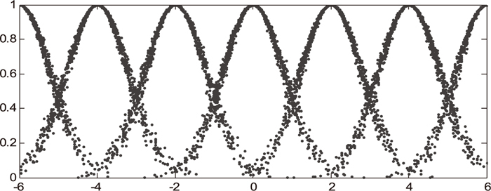
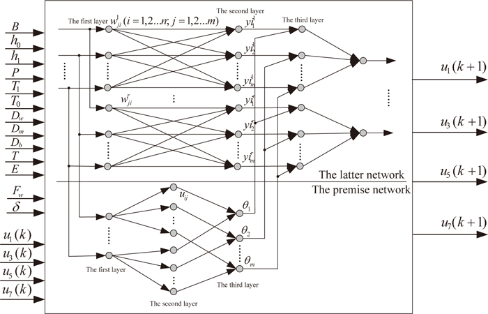
In this paper, cloud model is utilized to replace the Gauss membership function. The shape and distribution of cloud membership function is shown in Fig. 3. Based on above, T-S cloud inference neural network is constructed. The structure of T-S cloud inference network is shown in Fig. 4. It has two parts: the premise network and the latter network. The premise network is used for matching the premise of cloud fuzzy rules, and the latter network is used for generating the latter of cloud fuzzy rules.

Fig. 3.

Shape and distribution of cloud membership function.

Fig. 4.

The structure of T-S cloud inference network.

The premise network has three layers:

The first layer is input layer, the input variables are introduced into the premise network through it. It has n codes.

The second layer is cloud layer. Each node represents a cloud model and the input variables are clouded in this layer. Each input variable is clouded into m parts. The number of nodes is n × m. A node in this layer is shown in Fig. 5.

Fig. 5.

A node in the second layer.

The third layer is cloud inference layer. Each node represents a cloud fuzzy rule. The output of the premise network corresponds to the fitness value of a cloud fuzzy rule. It is usually represented by algebraic product:   

$${\theta }_j=u_{1j}\cdot u_{2j}\cdot \cdot \cdot u_{nj}=\prod _{i=1}^n{u}_{ij},j=1,2,\cdot \cdot \cdot ,m$$(3)

There are m nodes in this layer.

The latter network has three layers:

The first layer is input layer, and the input variables are transported to the second layer. In this layer, x₀ = 1 is used to provide the constant term for the latter of cloud fuzzy rule.

The second layer has m nodes. Each node represents a rule and it is used to calculate the latter of each rule. The outputs:   

$$y{i}_j^k=\sum _{i=0}^n{x}_i\cdot w_{ji}^k\mathrm{\hspace{0.17em} }\mathrm{\hspace{0.17em} }\mathrm{\hspace{0.17em} }\mathrm{\hspace{0.17em} }\mathrm{\hspace{0.17em} }\mathrm{\hspace{0.17em} }\mathrm{\hspace{0.17em} }(x_0=1)\mathrm{\hspace{0.17em} }\mathrm{\hspace{0.17em} }$$(4)

Where k = 1,2, ···, r; j = 1,2, ···, m.

The third layer is to calculate the total output of the network:   

$$y_k=\frac{\sum _{j=1}^m{\theta }_j\cdot y{i}_j^k}{\sum _{j=1}^m{\theta }_j}$$(5)

2.3. Optimize the Network by GA

When the p sample inputs network, the error for each sample is the square sum of each output error:   

$$E_p=\frac{1}{2}\sum _{k=1}^r{\left(d_k-y_k\right)}^2$$(6)

Where d_k is desired output.

After all the learning sample inputs network, the total error:   

$$E=\sum _{t=1}^q{E}_p=\frac{1}{2}\sum _{t=1}^q\sum _{k=1}^r{\left(d_k-y_k\right)}^2$$(7)

Where q is the count of samples.

GA is an efficient, parallel, global search method. It imitates the biological genetic and evolutionary mechanisms which roots in Darwin’s evolution theory and Mendel’s genetics. The algorithm can automatically obtain the search process and accumulate knowledge of the search space, and adaptively control the search process so as to achieve the optimal solution. In this paper, GA is applied to optimize T-S cloud inference neural network. Equation (7) is selected as fitness function. A mass of samples are used for training the network. When He is determined, the parameters to be optimized in the network are Ex, En and the weight w in the latter network.

2.4. Stability Analysis of T-S Cloud Inference Neural Network

In general, a multiple outputs system can be broken up into many single output systems. So, multiple outputs T-S cloud inference neural network can be broken up into many single output T-S cloud inference neural networks. Single output network is analyzed firstly. Then, the method can be popularized for multiple outputs T-S cloud inference neural network.

The discrete cloud fuzzy model of multiple inputs single output T-S cloud inference neural network is:   

$$\begin{array}{l}{R}^i:\mathrm{\hspace{0.17em} }if\mathrm{\hspace{0.17em} }{x}_k\mathrm{\hspace{0.17em} }is\mathrm{\hspace{0.17em} }{A}_1^i\mathrm{\hspace{0.17em} }and\mathrm{\hspace{0.17em} }{x}_{k-1}\mathrm{\hspace{0.17em} }is\mathrm{\hspace{0.17em} }{A}_2^i\mathrm{\hspace{0.17em} }and\cdots and\mathrm{\hspace{0.17em} }{x}_{k-n+1}\mathrm{\hspace{0.17em} }is\mathrm{\hspace{0.17em} }{A}_n^i\\ \mathrm{\hspace{0.17em} }\mathrm{\hspace{0.17em} }\mathrm{\hspace{0.17em} }\mathrm{\hspace{0.17em} }\mathrm{\hspace{0.17em} }then\mathrm{\hspace{0.17em} }{x}_{k+1}={\omega }_1^i{x}_k+{\omega }_2^i{x}_{k-1}+\cdots +{\omega }_n^i{x}_{k-n+1}\end{array}$$

Where: Rⁱ (i = 1, 2, …, m) represents the i th cloud fuzzy rules, and m is the total. x_k, x_k–1, …, x_k–n+1 are the state variable of system. A is the cloud fuzzy set of state variable. It is the cloud model. x_k+1 is the output of the second layer in the latter network. ω is the weight of the latter network.²¹⁾ The equation can be written in matrix form:   

$$x(k+1)=W\cdot x(k)$$(8)

Where: x(k) ∈ Rⁿ, W ∈ Rⁿ × Rⁿ, x(k) = [x_k, x_k–1, …, x_k–n+1]^T,   

$$W=\left(\begin{array}{ccccc}{\omega }_1^i& {\omega }_2^i& \cdots & {\omega }_{n-1}^i& {\omega }_n^i\\ 1& 0& \cdots & 0& 0\\ 0& 1& \cdots & 0& 0\\ ⋮& ⋮& \ddots & ⋮& ⋮\\ 0& 0& \cdots & 1& 0\end{array}\right)$$

Total output of the network is:   

$$X(k+1)=\sum _{i=1}^m{\theta }_i\cdot W\cdot x(k)\stackrel{}{}/\underset{}{}\sum _{i=1}^m{\theta }_i$$(9)

θ_i is the fitness of the i th cloud fuzzy rule:   

$${\theta }_i=\prod _{j=1}^n{\mu }_{ij}(x_{k-j+1})$$

So, θ_i is the function of x(k). Let θ_i = g_i[x(k)], G[x(k)] is:   

$$\begin{array}{l}G[x(k)]=\frac{\sum _{i=1}^m{\theta }_i\cdot W}{\sum _{i=1}^m{\theta }_i}\\ =\left(\begin{array}{ccccc}\frac{\sum _{i=1}^m{\omega }_1^i{g}_i}{\sum _{i=1}^m{g}_i}& \frac{\sum _{i=1}^m{\omega }_2^i{g}_i}{\sum _{i=1}^m{g}_i}& \cdots & \frac{\sum _{i=1}^m{\omega }_{n-1}^i{g}_i}{\sum _{i=1}^m{g}_i}& \frac{\sum _{i=1}^m{\omega }_n^i{g}_i}{\sum _{i=1}^m{g}_i}\\ 1& 0& \cdots & 0& 0\\ 0& 1& \cdots & 0& 0\\ ⋮& ⋮& \ddots & ⋮& ⋮\\ 0& 0& \cdots & 1& 0\end{array}\right)\end{array}$$

Then, multiple inputs single output T-S cloud inference neural network is:   

$$X(k+1)=G[x(k)]\cdot x(k)$$(10)

Equation (10) is a state equation of matrix form of nonlinear discrete system, and only the first line of state matrix is effective. Then,   

$$X(k+1)=\frac{\sum _{i=1}^m{\omega }_1^i{g}_i}{\sum _{i=1}^m{g}_i}{x}_k+\frac{\sum _{i=1}^m{\omega }_2^i{g}_i}{\sum _{i=1}^m{g}_i}{x}_{k-1}+\cdots +\frac{\sum _{i=1}^m{\omega }_n^i{g}_i}{\sum _{i=1}^m{g}_i}{x}_{k-n+1}$$(11)

Because the expression of each cloud model is not a single one in the whole domain space. It is a piecewise function divided by the value of x. So G[x(k)] is a piecewise polynomial matrix. It is hard to analyze the stability directly. For the system, there exists an area Ω₁ around the balance point. In the area Ω₁, each cloud model can be unified to one expression. So, G[x(k)] is a single expression in this area. And it is used to judge the stability of the network. Because of the area Ω₁, x(k) is seen as the constant. So, the whole system is transformed into a linear time-invariant discrete system.²²⁾   

$$\begin{array}{l}X(k+1)=G[x(k)]\cdot x(k)\\ =\left(\begin{array}{ccccc}\frac{\sum _{i=1}^m{\omega }_1^i{g}_i}{\sum _{i=1}^m{g}_i}& \frac{\sum _{i=1}^m{\omega }_2^i{g}_i}{\sum _{i=1}^m{g}_i}& \cdots & \frac{\sum _{i=1}^m{\omega }_{n-1}^i{g}_i}{\sum _{i=1}^m{g}_i}& \frac{\sum _{i=1}^m{\omega }_n^i{g}_i}{\sum _{i=1}^m{g}_i}\\ 1& 0& \cdots & 0& 0\\ 0& 1& \cdots & 0& 0\\ ⋮& ⋮& \ddots & ⋮& ⋮\\ 0& 0& \cdots & 1& 0\end{array}\right)x(k)\end{array}$$

The eigenvalues of G[x(k)] in unit circle $\Vert z\Vert =1$ is necessary and sufficient conditions of stability. In the area Ω₁, if every eigenvalue is located in unit circle, then the value range of x(k) will be determined. It is the stability area Ω₂.

When the rank of G[x(k)] is above three. Lyapunov method is utilized to analyze the stability of the network: for any given positive definite symmetric Q, there must exist a positive definite symmetric P, they satisfy:   

$$G^{T}PG-P=-Q$$

Let:   

$$Q=I=\left(\begin{array}{cccc}1& 0& \cdots & 0\\ 0& 1& \cdots & 0\\ ⋮& ⋮& \ddots & ⋮\\ 0& 0& \cdots & 1\end{array}\right)$$

If P is positive, the value range of x(k) and the stability area Ω₂ will be obtained.

If above method is used to analyze the stability, an extra condition should be satisfied: when x(k) is located in area Ω₃, X(k + 1) should be located in the same area. Under this condition, G[x(k)] is a constant matrix. When:   

$$\begin{array}{c}\left|x_{k-i}\right|\le M\mathrm{\hspace{0.17em} }(i=0,1,2,\dots ,n-1)\hspace{1em}\\ \left|X(k+1)\right|\le M\end{array}$$(12)

Where M is a constant. The task is to find the area Ω₃. If   

$$\left|x_{k-i}\right|\le M\mathrm{\hspace{0.17em} }(i=0,1,2,\dots ,n-1),$$

then   

$$\begin{array}{l}\left|X(k+1)\right|=\left|\frac{\sum _{i=1}^m{\omega }_1^i{g}_i}{\sum _{i=1}^m{g}_i}{x}_k+\frac{\sum _{i=1}^m{\omega }_2^i{g}_i}{\sum _{i=1}^m{g}_i}{x}_{k-1}+\cdots +\frac{\sum _{i=1}^m{\omega }_n^i{g}_i}{\sum _{i=1}^m{g}_i}{x}_{k-n+1}\right|\\ \le \left|\frac{\sum _{i=1}^m{\omega }_1^i{g}_i}{\sum _{i=1}^m{g}_i}{x}_k\right|+\left|\frac{\sum _{i=1}^m{\omega }_2^i{g}_i}{\sum _{i=1}^m{g}_i}{x}_{k-1}\right|+\cdots +\left|\frac{\sum _{i=1}^m{\omega }_n^i{g}_i}{\sum _{i=1}^m{g}_i}{x}_{k-n+1}\right|\\ \le \left|\frac{\sum _{i=1}^m{\omega }_1^i{g}_i}{\sum _{i=1}^m{g}_i}\right|\cdot \left|x_k\right|+\left|\frac{\sum _{i=1}^m{\omega }_2^i{g}_i}{\sum _{i=1}^m{g}_i}\right|\cdot \left|x_{k-1}\right|+\cdots +\left|\frac{\sum _{i=1}^m{\omega }_n^i{g}_i}{\sum _{i=1}^m{g}_i}\right|\cdot \left|x_{k-n+1}\right|\\ \le \left|\frac{\sum _{i=1}^m{\omega }_1^i{g}_i}{\sum _{i=1}^m{g}_i}\right|\cdot M+\left|\frac{\sum _{i=1}^m{\omega }_2^i{g}_i}{\sum _{i=1}^m{g}_i}\right|\cdot M+\cdots +\left|\frac{\sum _{i=1}^m{\omega }_n^i{g}_i}{\sum _{i=1}^m{g}_i}\right|\cdot M\\ =\left(\left|\frac{\sum _{i=1}^m{\omega }_1^i{g}_i}{\sum _{i=1}^m{g}_i}\right|+\left|\frac{\sum _{i=1}^m{\omega }_2^i{g}_i}{\sum _{i=1}^m{g}_i}\right|+\cdots +\left|\frac{\sum _{i=1}^m{\omega }_n^i{g}_i}{\sum _{i=1}^m{g}_i}\right|\right)\cdot M\end{array}$$

When   

$$\left|\frac{\sum _{i=1}^m{\omega }_1^i{g}_i}{\sum _{i=1}^m{g}_i}\right|+\left|\frac{\sum _{i=1}^m{\omega }_2^i{g}_i}{\sum _{i=1}^m{g}_i}\right|+\cdots +\left|\frac{\sum _{i=1}^m{\omega }_n^i{g}_i}{\sum _{i=1}^m{g}_i}\right|\le 1$$(13)

, then   

$$\left|X(k+1)\right|\le M$$

Apparently, Eq. (13) is conservative. In a real world application, the value range of x(k) is obtained flexibly according to Eq. (11). On the basis of Lyapunov system stability definition, the network is asymptotic stability in Ω₃. So, the stability area is Ω₂ ∩ Ω₃.

To sum up, the stability analysis of multiple inputs single output T-S cloud inference neural network is obtained. The same method can be used to analyze multiple inputs multiple outputs T-S cloud inference neural network.

3. Flatness Control System Design

This paper takes 6-high 900HC reversible cold rolling mill as research object. Based on T-S cloud inference neural network, a closed-loop flatness control system which consists of flatness pattern recognition model, flatness predictive model and flatness controller is designed. The control methods are working roll bending and middle roll shifting. The structure of flatness control system is shown in Fig. 6, and the flow chart of control system is shown in Fig. 7.

Fig. 6.

Structure of flatness control system.

Fig. 7.

The flow chart of flatness control system.

3.1. Flatness Pattern Recognition Model

Flatness pattern recognition is a basic part of flatness control.²³⁾ In consideration of the diversity of control method and the requirement of precise control, right-one-third waves and left-one-third waves were introduced on the basis of traditional six basic patterns. So, there are eight common flatness recognition signal basic patterns: left waves, right waves, center waves, double-edge waves, right-one-third waves, left-one-third waves, quarter waves and edge-center waves.^24,25,26) The flatness rolled can be formulated as linear combination of basic patterns:²⁷⁾   

$$f(y)=u_1{p}_1\left(y\right)+u_3{p}_2\left(y\right)+u_5{p}_3\left(y\right)+u_7{p}_4\left(y\right)$$(14)

Where:   

$$p_1\left(y\right)=y,\mathrm{\hspace{0.17em} }{p}_2\left(y\right)=\frac{3}{2}{y}^2-\frac{1}{2}$$

  

$$p_3\left(y\right)=\frac{1}{2}\left(5y^3-3y\right),\mathrm{\hspace{0.17em} }{p}_4\left(y\right)=\frac{1}{8}\left(35y^4-30y^2+3\right)$$

p₁(x), p₂(x), p₃(x), p₄(x) represent linear, quadratic, cubic, quartic Legendre polynomial expansion. u₁, u₃, u₅, u₇ represent membership degree of flatness deviation. The value reflects the content of each shape deviation, and the symbol reflects the pattern of flatness. When the value is positive, it represents left waves, center waves, right-one-third waves and quarter waves; when the value is negative, it represents right waves, double-edge waves, left-one-third waves and edge-center waves. Suppose the measured flatness stress value to be identified are normalized as: Y = [σ(1), σ(2), …, σ(m)]. The k th basic pattern is: Y_k = [σ_k(1), σ_k(2), ···, σ_k(m)] (k = 1,2···8). m is the amount of measuring section.

The Euclidean distance is regard as the model input in flatness pattern recognition. The Euclidean distance between Y and Y_k is:   

$$D_k=\Vert Y-Y_k\Vert =\sqrt{\sum _{i=1}^n{[\sigma (i)-{\sigma }_k(i)]}^2}\hspace{1em}\hspace{1em}k=1,2,\cdots ,8$$(15)

According to the requirements of rolling mill implementing agency, left waves and right waves, center waves and double-edge waves, right-one-third waves and left-one-third waves, quarter waves and edge-center waves cannot exist at the same time in the flatness basic pattern identified.²⁸⁾ D_k is processed as follows:

If D₁ < D₂, then d₁ = D₁, otherwise d₁ = –D₂;

If D₃ < D₄, then d₂ = D₃, otherwise d₂ = –D₄;

If D₅ < D₆, then d₃ = D₅, otherwise d₃ = –D₆;

If D₇ < D₈, then d₄ = D₇, otherwise d₄ = –D₈.

The model of flatness pattern recognition is a four-input and four-output system. The flatness pattern recognition model based on T-S cloud inference neural network is shown in Fig. 8. d_j(j = 1, 2, 3, 4) is the input and u_j(j = 1, 3, 5, 7) is the output.

Fig. 8.

The flatness pattern recognition model.

3.2. Rolling Mill Flatness Predictive Model

In order to improve the predictive accuracy, factors of affecting flatness are taken into consideration as many as possible, and the number is selected as seventeen. The basic rolling parameters: initial width of strip B, entrance average thickness h₀, exit average thickness h₁, rolling pressure P, front tension T₁, back tension T₀, work roll diameter D_w, intermediate roll diameter D_m, backup roll diameter D_b, rolling temperature T, Young’s modulus of elasticity E; The flatness adjustment parameters: work roll bending force F_w, intermediate roll shifting position δ; The flatness membership degree of k moment: u₁(k), u₃(k), u₅(k), u₇(k). The outputs of predictive model are flatness membership degree of k + 1 moment: u₁(k + 1), u₃(k + 1), u₅(k + 1), u₇(k + 1). Then, a seventeen inputs four outputs flatness predictive model is constructed by T-S cloud inference neural network. The inputs and outputs are shown as follows: inputs:   

$$\begin{array}{c}U=[B,h_0,h_1,P,T_1,T_0,D_w,D_m,D_b,T,E,F_w,\\ \delta ,u_1(k),u_3(k),u_5(k),u_7(k){]}^T\end{array}$$

outputs:   

$$Y={[u_1(k+1),u_3(k+1),u_5(k+1),u_7(k+1)]}^T$$

The structure of flatness predictive model is shown in Fig. 9.

Fig. 9.

The structure of flatness predictive model.

3.3. Flatness Controller Design

Based on T-S cloud inference neural network, the flatness T-S cloud inference controller is designed. It is a four-input and two-output controller. The inputs are the subtraction of target flatness characteristic value and rolling mill flatness membership degree. The outputs are work roll bending force F_w and intermediate roll shifting position δ. The structure of T-S cloud inference controller is shown in Fig. 10.

Fig. 10.

The structure of T-S cloud inference controller.

Initial parameters of the controller are firstly determined through offline training based on measured data by 900HC reversible cold rolling mill. Then, the controller is applied for flatness control system and it is shown in Fig. 6. GA is utilized to optimize the controller parameters online. According to the structure of T-S cloud inference controller, there are 72 variables need to be optimized. In order to make it more convenient, GA toolbox and real number coding method were used. The parameters of GA mainly include population size, stopping generations, crossover probability and mutation probability. These parameters need to be preset: population size is 20; stopping generations are 400; crossover probability is 0.8; mutation probability is 0.2. The optimization objective is to get the minimum of fitness value. Fitness value and current best individual are shown in Figs. 11 and 12.

Fig. 11.

The fitness value.

Fig. 12.

The current best individual.

4. Simulation Results and Discussions

In order to test the effectiveness of the method proposed above, T-S cloud inference neural network is applied for 900HC reversible cold rolling mill. For a kind of steel strip, the rolling specification is: 2.2×662→0.247×662 and the material is SPHC. The rolling basic parameters are shown in Table 1. The experiment samples are all measured continuous data from a steel rolling factory.

Table 1. The basic rolling parameters.

Basic input parameters	Value range
Initial width of strip B (mm)	460–480
Entrance average thickness h0 (mm)	0.24–4.0
Exit average thickness h1 (mm)	0.24–1.5
Rolling pressure P (MPa)	0–13
Front tension T1 (N)	4000–80000
Back tension T0 (N)	4000–80000
Work roll diameter Dw (mm)	245–270
Intermediate roll diameter Dm (mm)	320–340
Backup roll diameter Db (mm)	790–850
Rolling temperature T (°C)	55–56
Young’s modulus of elasticity E (MPa)	21000
Work roll bending force Fw (T)	–25.969–40.8
Intermediate roll shifting position δ (mm)	–200–200

4.1. Simulation Test One

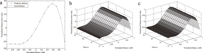
Based on T-S cloud inference neural network, flatness predictive model is established. And training samples are normalized. At the exit of first, third and fifth pass, 900HC reversible cold rolling mill is equipped with flatness meter. Then, the predictive flatness is compared with the measured flatness in first, third and fifth pass. The results are shown in Table 2. SSE stands for the square sum of error between predictive outputs and actual outputs. In order to be more lively and clear, flatness three-dimensional diagrams for a moment are shown in Figs. 13, 14 and 15.

Table 2. The results of predictive flatness and actual flatness.

Pass	Predictive outputs	Actual outputs	SSE
First pass	u1 = 0.6404	u1 = 0.6415	0.0016
	u3 = –0.162	u3 = –0.1489
	u5 = –0.5683	u5 = –0.6084
	u7 = –0.3132	u7 = –0.3012
Third pass	u1 = 0.8716	u1 = 0.87	0.000102
	u3 = –0.2159	u3 = –0.212
	u5 = –0.786	u5 = –0.7809
	u7 = –0.168	u7 = –0.1604
Fifth pass	u1 = 0.6336	u1 = 0.6503	0.0022
	u3 = –0.0751	u3 = –0.1155
	u5 = –0.4773	u5 = –0.4736
	u7 = –0.2812	u7 = –0.2638

Fig. 13.

Flatness three-dimensional diagrams for a moment in first pass: (a) two-dimensional diagram of predictive flatness and actual flatness; (b) three-dimensional diagram of predictive flatness; (c) three-dimensional diagram of actual flatness.

Fig. 14.

Flatness three-dimensional diagrams for a moment in third pass: (a) two-dimensional diagram of predictive flatness and actual flatness; (b) three-dimensional diagram of predictive flatness; (c) three-dimensional diagram of actual flatness.

Fig. 15.

Flatness three-dimensional diagrams for a moment in fifth pass: (a) two-dimensional diagram of predictive flatness and actual flatness; (b) three-dimensional diagram of predictive flatness; (c) three-dimensional diagram of actual flatness.

From Table 2 and Figs. 13, 14, 15, it can be seen that the predictive flatness has good consistency to the actual flatness. The flatness predictive model established in this paper possesses preferable predictive ability. It provides the basis for flatness control.

4.2. Simulation Test Two

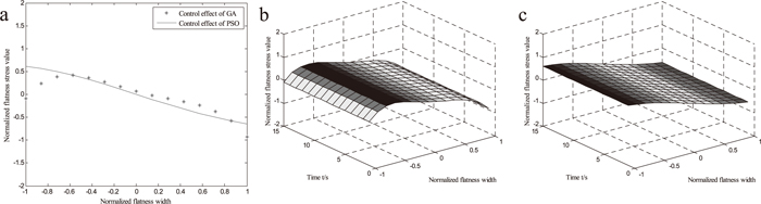
In order to show the control effect of the flatness control system, GA and PSO are utilized to train the controller and the flatness predictive model. The flatness control system is shown in Fig. 6. Under the environment of MATLAB 2010a, the control results of GA and PSO are shown in Table 3. For the sake of direct-viewing and convenience, flatness three-dimensional diagrams for a moment are shown in Figs. 16, 17 and 18.

Table 3. The control results of GA and PSO.

Pass	GA	PSO
First pass	u1 = 0.7623	u1 = 0.7105
	u3 = –0.486	u3 = –0.7022
	u5 = –0.4776	u5 = –0.2315
	u7 = –0.1141	u7 = –0.3541
Third pass	u1 = –0.5111	u1 = –0.6906
	u3 = –0.2928	u3 = –0.0103
	u5 = 0.0945	u5 = 0.0657
	u7 = –0.2153	u7 = –0.0064
Fifth pass	u1 = 0.1854	u1 = 0.5869
	u3 = –0.1051	u3 = 0.4714
	u5 = 0.1205	u5 = 0.1634
	u7 = –0.2997	u7 = –0.3394

Fig. 16.

Flatness three-dimensional diagrams for a moment in first pass: (a) two-dimensional diagram of GA and PSO control effects; (b) three-dimensional diagram of GA control effect; (c) three-dimensional diagram of PSO control effect.

Fig. 17.

Flatness three-dimensional diagrams for a moment in third pass: (a) two-dimensional diagram of GA and PSO control effects; (b) three-dimensional diagram of GA control effect; (c) three-dimensional diagram of PSO control effect.

Fig. 18.

Flatness three-dimensional diagrams for a moment in the fifth pass: (a) two-dimensional diagram of GA and PSO control effects; (b) three-dimensional diagram of GA control effect; (c) three-dimensional diagram of PSO control effect.

Table 2 and Figs. 16, 17, 18 illustrate that the control effect of GA and PSO. In Table 2, the output flatness membership degrees of GA in fifth pass are smaller than PSO. It indicates that the rolling flatness is more smooth and GA has a better control effect. In Fig. 18, the output flatness can be seen more intuitionally. In order to compare the control effect of two algorithms, the flatness curves of the first pass and the fifth pass are drawn in the same figure. It is shown in Fig. 19.

Fig. 19.

Flatness comparison curves.

Figure 19 illustrates the flatness comparison curves of the first pass and the fifth pass. In the same circumstances, the fifth pass flatness deviation compared with the first pass decreases 85.85 percent by T-S cloud inference controller based on GA. While, flatness deviation decreases 39.79 percent by T-S cloud inference controller based on PSO. It can be seen that T-S cloud inference controller based on GA is more superior. So, the flatness control system designed by T-S cloud inference neural network based on GA is an effective flatness control method and has a better precision. The training process is fast and it has a strong robustness.

5. Conclusions and Future Research

This paper proposes a new neural network, called T-S cloud inference neural network. It is a multiple inputs multiple outputs network. The cloud model is combined with T-S fuzzy neural network. The rapidity of fuzzy logic and the uncertainty of cloud model for processing data are both taken into account synthetically. The stability of the network is analyzed by Lyapunov method. And then, flatness pattern recognition model and flatness predictive model are established. By using T-S cloud inference controller, a flatness control system is constructed completely. The system is applied for 900HC reversible cold rolling mill. Simulation results demonstrate that GA is a better algorithm to optimize the T-S cloud inference neural network compared with PSO. It can make the flatness control system reach higher precision and better control effect. The flatness control system based on T-S cloud inference neural network optimized by GA is a new flatness control method. The future work will concentrate on flatness control system of the visual.²⁹⁾ The flatness control interface is utilized to simulate the whole rolling process. And the control results will be showed lively and convenient with pressing a button.

Acknowledgments

The authors wish to thank the anonymous reviewers for their constructive comments and suggestions. Those comments are all valuable and very helpful for revising and improving our paper, as well as the important guiding significance to our research. This work is supported by the National Natural Science Foundation of China (Grants No. 61074099) and Cultivation Program Project for Leading Talent of Innovation Team in Colleges and Universities of Hebei Province (No. LJRC013. Automation technology and application of continuous casting and steel rolling).

References

• 1)   Y.  Zhang,  Q.  Yang and  X.  Wang: J. Iron Steel Res. Int., 18 (2011), 27.
• 2)   H.  Liu,  H.  He and  X.  Shan: Chinese J. Mech. Eng., 22 (2009), 287.
• 3)   E.  Hatzikos,  L.  Anastasakis,  N.  Bassiliades and  I.  Vlahavas: Proc. 2nd Int. Scientific Conf. on Computer Science, IEEE Computer Society, Bulgarian Section, IEEE, Piscataway, NJ, (2005), 254.
• 4)   A.  Preis and  A.  Ostfeld: J. Hydrol., 34 (2008), 364.
• 5)   S.  Mahapatra,  S.  Nanda and  B.  Panigrah: Adv. Eng. Software, 42 (2011), 787.
• 6)   D.  Faruk: Eng. Appl. Artif. Intell., 23 (2010), 586.
• 7)   G.  Tan,  J.  Yan,  C.  Gao and  S.  Yang: Proc. Eng., 31 (2012), 1194.
• 8)   X.  Zhang: China Mech. Eng., 18 (2007), 2419.
• 9)   J.  Wang and  H.  Li: Mach. Tool Hydraulic., 35 (2007), 152.
• 10)   X.  Shan,  C.  Jia and  H.  Liu: J. Mech. Eng., 45 (2009), 255.
• 11)   C.  Jia,  Y.  Cui and  D.  Xu: Metall. Equipment, 6 (2010), 1.
• 12)   W.  Fan: Metall. Power, 5 (2012), 80.
• 13)   F.  Zhang,  Y.  Fan and  C.  Shen: Control Theor. Appl., 17 (2000), 519.
• 14)   B.  Liu and  H.  Li: Comput. Appl., 28 (2008), 305.
• 15)   Z.  Xu and  Z.  Fan: Acta Armamentarii, 6 (2009), 727.
• 16)   S.  Gan,  H.  Liu and  Z.  Shen: Control Eng. China, 12 (2005), 442.
• 17)   P.  Wang and  X.  Zhang: Comput. Eng. Appl., 45 (2009), 246.
• 18)   X.  Zhou,  W.  Jiang and  L.  Ma: Power Syst. Prot. Contr., 38 (2010), 37.
• 19)   H.  Zhu,  F.  Wang,  Y.  Zhang and  F.  Zhang: Math. Practice Theory, 43 (2013), 117.
• 20)   D.  Li and  Y.  Du: Uncertainty Artificial Intelligence, National Defence Industry Press, Beijing, (2005), 143.
• 21)   F.  Wu,  Z.  Shi and  G.  Dai: Control Decision, 14 (1999), 65.
• 22)   K.  Tanaka and  M.  Sugeno: Fuzzy Set Syst., 145 (1992), 135.
• 23)   H.  Tseng: J. Intell. Manuf., 17 (2006), 301.
• 24)   X.  Shan,  H.  Liu and  C.  Jia: Iron Steel, 45 (2010), 56.
• 25)   C.  Jia,  X.  Shan and  H.  Liu: J. Iron Steel Res. Int., 15 (2008), 33.
• 26)   X.  Zhang,  S.  Zhang,  G.  Tan and  W.  Zhao: J. Iron Steel Res. Int., 19 (2012), 25.
• 27)   H.  He and  N.  Li: Process Automat. Instr., 28 (2007), 1.
• 28)   J.  Jung: Mater. Process. Technol., 63 (1997), 248.
• 29)   X.  Zhang,  L.  Zhao,  J.  Zang,  H.  Fan and  L.  Cheng: Steel Res. Int., 85 (2014), 1.