Instability and Periodicity of Asymmetrical Flow in a Funnel Thin Slab Continuous Casting Mold

Abstract

Characteristics of the transient turbulent flow in a funnel thin slab continuous casting mold are studied using a large eddy simulation (LES) computational approach. Validations were done through comparison with previous experimental data of the mean velocities and the instantaneous velocities, and good qualitative and quantitative agreements are obtained. The turbulence flow inside the mold consists of various scales vortices; many pronounced large scale vortex structures were clear found inside the mold, containing various small scale vortices between them. The boundary shear flow can separate from the narrow wall and transport vorticity into the interior flow, and then possibly develop into a vortex. The intermittent chaotic vortex formation on both sides of the SEN is found at the meniscus. Three types of vortex phenomena are identified: one big vortex, two vortices and three small vortices. The positions and sizes are different, and the vortexes are located at the low velocity sides adjacent to the SEN. Significant asymmetry is seen in the instantaneous flow in the two halves of the thin slab mold cavity, especially in the lower recirculation zone. The periodical behavior of asymmetric flow inside the liquid pool was identified and characterized. The spectrum of velocities shows that the mean time interval for periodical changeover is 14.28 seconds.

1. Introduction

Near-net-shape casting^1,2) of flat products is one of the true technological adventures that the steel industry has undertaken in the last 30 years. As an important commercial near-net-shape casting technology, thin slab continuous casting (TSCC) process^3,4,5) has been developed rapidly and used widely to reduce production cost and the amount of scrap and improve productivity in steel industry. One significant feature of TSCC, different from that of conventional slab casting, is the use of the funnel-type mold, which provides the necessary space for the submerged entry nozzle (SEN) to conduct molten steel into the thin slab mold. Due to the high casting speed and high width to thickness ratio for thin slab caster, the molten steel flows inside the mold with intense turbulence. The turbulence flow^6,7,8) of molten steel plays a key role in slab quality since it influences the solidification procedure, mold powder entrapment and the floatation of non-metallic inclusions. Therefore, control and optimization of the turbulent flow play an important role in attaining a better product quality.

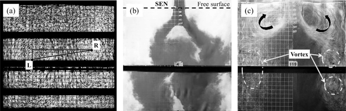
According to recent plant observations and detections, the distribution of argon bubbles and non-metallic inclusions captured by solidified shell in the rolled steel plates was intermittent and asymmetric;^8,9,10) suggesting that the fluid flow inside the mold was unsteady and instable. Several physical modeling studies^{8,10,11,12,13,14,15,16,17)} have been carried out to reproduce the asymmetrical and oscillating fluid flow inside the casting mold. Gupta et al.^11,12) found that the flow pattern in the lower recirculation zone of a traditional slab mold was asymmetric and oscillating about the central plane with a random period. They hypothesized that the origin of the asymmetrical flows was due to a swirl cycle when the jets hit the wide face of the mold and then the flow goes up or down below the SEN port level. Honeyands et al.¹³⁾ investigated the time dependent flow phenomena in a 1:6 scale water model of thin slab caster, and observed that the fluid flow pattern were neither steady nor symmetric, instead oscillated periodically. Shen et al.¹⁴⁾ studied the instability of fluid flow and level fluctuation in a full scale water model of thin slab caster; found that the internal fluid flow and level fluctuation were unsteady and periodical. Figure 1(a) shows the flow pattern inside their water model using the particle image visualization method, it can be seen that the positions of the two vortex cores were asymmetric. Wang et al.¹⁵⁾ performed another full scale water model to investigate the transient asymmetrical fluid flow inside a thin slab mold without and with air injection, respectively, as shown in Figs. 1(b) and 1(c). A periodical level fluctuation had been found in their water experiments, as called meniscus dynamic distortion (MDD). Recently, Torres-alonso et al.¹⁶⁾ studied the cyclic turbulent instabilities in a thin slab mold using a water-physical model of a funnel-type thin slab mold, a low-frequency and energetic flow distortion was identified. And a theoretical hypothesis was proposed to explain the origins of the dynamic distortion on a temporal unbalance of the turbulent kinetic energy.

Fig. 1.

Flow pattern inside different thin slab molds obtained from previous works (a) particle image visualization;¹⁴⁾ (b) dye tracer;¹⁵⁾ and (c) bubble tracer.¹⁵⁾

Experimental measurements on an actual thin slab continuous casting machine are very difficult, dangerous and expensive. Numerical modeling provides an alternative tool to understand and solve this kind of problem. Most of the reported mathematical models have been performed using the Reynolds averaged Navier-Stokes (RANS) models,^18,19,20,21) such as the k-ε or Reynolds stresses. These models predict time-averaged velocities with reasonable accuracy and at a reasonable computational. However, these models, limited by the RANS’s nature, are not suited for modeling the evolution of transient flow pattern triggered by flow instabilities. As shown in Fig. 2, obtained from the k-ε model, the predicted flow pattern inside the present calculation mold was symmetric and stable, failure to explain the asymmetrical and oscillating fluid flow inside the mold. In recent studies,^8,10,22,23) the large eddy simulation (LES) has been successfully applied to obtain the transient asymmetrical flow inside the mold. Yuan et al.²²⁾ combined LES and particle image velocimetry (PIV) measurements in a scaled water model, finding good agreement between both types of data. Many transient phenomena have been observed using LES and PIV measurement?which RANS model cannot simulate. The asymmetric flow was found between the two rolls in the lower recirculation region, which was important for the inclusion motion and bubble entrapment. Ramos-Banderas et al.²³⁾ studied the fluid flow of water in a slab mold using LES and PIV, founding the asymmetrical flow and the flow pattern changed with time as a consequence of the vertical oscillation of the jet core. Recently, authors developed different LES models for the single phase (molten steel) flow⁸⁾ and the two-phase (molten steel and argon gas) flow¹⁰⁾ inside the slab mold, respectively. Both of simulation results agree acceptably well with the water model experimental measurements of instantaneous flow structures. The flow pattern in the lower recirculation zone is asymmetric and changeover; the direction of flow deviation is different from time to time. However, relatively little work has been reported on the periodicity of the asymmetrical flow in the funnel thin slab caster using LES. This information is important for finding some effective methods to improve the quality of steel product.

Fig. 2.

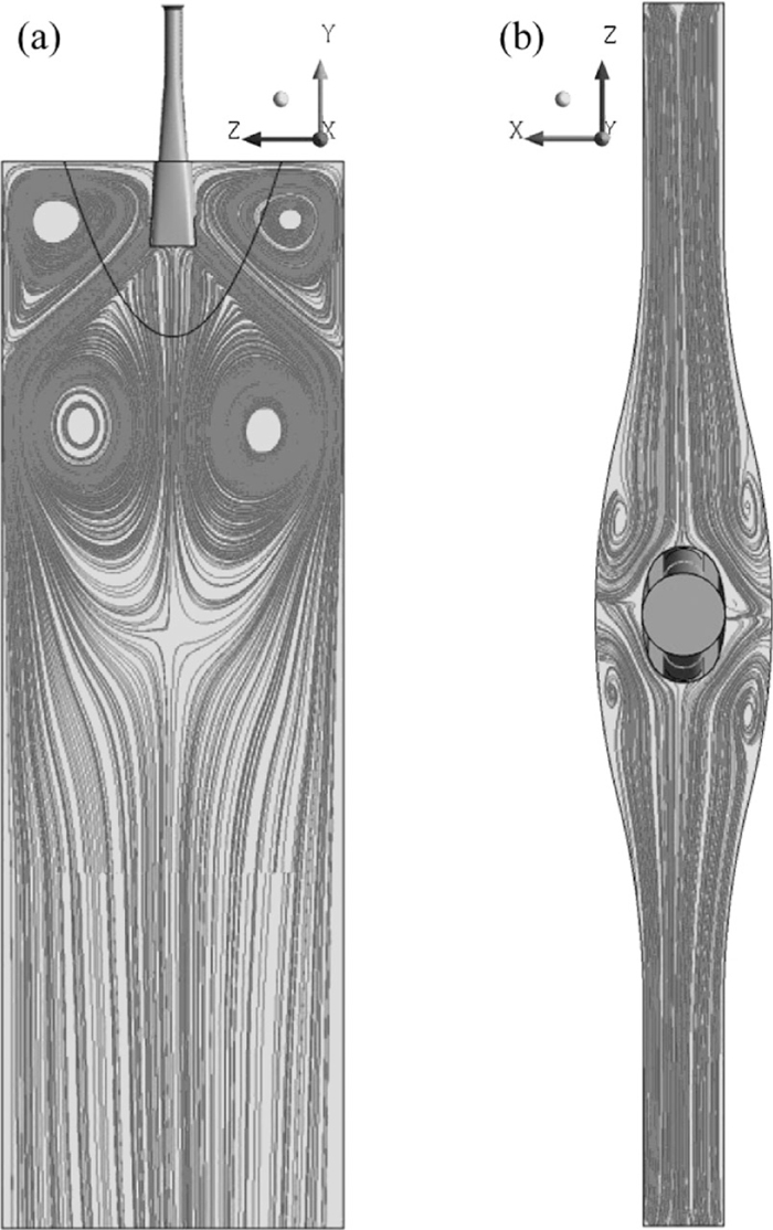
Typical steady flow pattern obtained from RANS model at the center plane between wide faces (a) and 10 mm below the top surface (b) (Case A1 in Table 1).

In this work, the instability and periodicity behaviors of the asymmetrical flow in a funnel thin slab caster are analyzed using LES model. Comparisons with previous measurements^22,24,25) are made where available, including velocities along the flow jet, below the top surface, and some monitoring points. The complex vorticity fields and asymmetrical flow patterns inside the mold and the various vortices on the top surface are obtained by this model. To accomplish the dynamic analysis of the turbulence flow inside the mold, 5 given monitoring points were defined. The periodic frequencies of the asymmetrical flow are analyzed through a frequency analysis of several velocity magnitude time series on these points.

2. Model Formulation

Turbulence flow is characterized by eddies with a wide range of length and time scales. The largest eddies are typically comparable in size to the characteristic length of the mean flow. The smallest scales are responsible for the dissipation of turbulence kinetic energy. In the context of LES, the large-scale eddies are resolved directly in the simulation. However, the small-scale eddies are less dependent on the geometry, tend to be more isotropic. So the dissipative effect of the small-scale eddies is represented using a sub-grid scale (SGS) model.

2.1. Governing Equation

The governing equations employed for LES are obtained by filtering the time-dependent Navier-Stokes equations. The filtering process effectively filters out the eddies whose scales are smaller than the filter width (grid size) used in the computations.

A filtered variable is defined by:   

$$f(x)={\int }_{D}f(x^{\prime })G(x,x^{\prime })d{x}^{\prime }$$(1)

where D is the fluid domain, and G(x, x′) is the filter function that determines the scale of the resolved eddies.

The cassette filter function²³⁾ was used in this work, G(x, x′) can be expressed as:   

$$G(x,x^{\prime })=\{\begin{array}{l}1/V,\begin{array}{cc}& if\left|x-x^{\prime }\right|<V/2\end{array}\\ 0\stackrel{}{},\begin{array}{cc}& otherwise\end{array}\end{array}$$(2)

where V = ΔxΔyΔz is the volume of a computational cell.

Filtering the Navier-Stokes equations, the resulting equations thus govern the dynamics of large eddies as:   

$$\begin{array}{l}\frac{\partial u_i}{\partial x_i}=0\\ \frac{\partial u_i}{\partial t}+\frac{\partial (u_i{u}_j)}{\partial x_j}=-\frac{1}{\rho }\frac{\partial p}{\partial x_i}+\nu {\nabla }^2{u}_i+\frac{\partial {\tau }_{ij}}{\partial x_j}\end{array}$$(3)

where u, t, P, ρ, v, and τ_ij is filtered velocity, time, pressure, density, kinematic viscosity, and sub-grid scale stress. The subscripts i and j represent the three Cartesian directions and repeated subscripts imply summation.

To model the dissipative effect of the small-scale eddies, the Smagorinsky SGS model²⁶⁾ is employed in this work. The sub-grid scale stress τ_ij is defined by:   

$${\tau }_{ij}=2{\mu }_t{S}_{ij}$$(4)

where μ_t and S_ij are the turbulent viscosity and rate-of-strain tensor for the resolved scale, respectively, and are defined as follows:²⁷⁾   

$${\mu }_t=\rho {(C_{S}L)}^2{(2S_{ij}{S}_{ij})}^{1/2}$$(5)

  

$$S_{ij}=\frac{1}{2}\left(\frac{\partial u_i}{\partial x_j}+\frac{\partial u_j}{\partial x_i}\right)$$(6)

where C_s is the Smagorinsky constant, C_s = 0.1; L is the mixing length for sub-grid scales, L = V^1/2.

2.2. Computational Details

The computational domain of this funnel thin slab mold includes the entire SEN, the complete mold region and extended part. Figure 3 schematically shows the important geometry structures and parameters for this computational model. The main characteristic of this mold is the funnel shaped design with an enlarged opening in the upper part of the mold, as shown in Fig. 3(E), which is the actual mold. The maximum thickness of the funnel-type casting area is 190 mm, and the height is 850 mm. As the molten steel travels through the downwardly converging funnel-type casting area, funnel thickness directly diminishes to the extent (70 mm) that it is equal to the thickness of the actual mold. The geometrical, physical properties and operating conditions used in numerical simulation model are shown in Table 1 (Case A1).

Fig. 3.

Schematics of the computational thin slab mold model (Case A1 in Table 1).

Table 1. Simulation conditions for different flow models.

Parameters	Case A1	Case A224)	Case A325)	Case A422)
Width of mold, m	1.53	1.93	1.32	0.735
Thickness of mold, m	0.07	0.229	0.22	95(top) to 65(bottom)
Length of mold, m	4.8	2.152	3.0	0.95
SEN submergence depth, m	0.2	0.1778	0.265	0.075
SEN outport angle, (°)	45 down	25 down	15 down	15 down
SEN outport sizes, mm	Special port	Circular port, 51	Rectangular port, 38 × 60	Rectangular port, 32 × 31
Casting speed, m/s	0.0917	0.0152	0.0167	0.0102
Density of fluid, kg/m3	7020	1000	1000	1000
Viscosity of fluid, N·s/m2	0.0064	0.001	0.001	0.001

A constant velocity inlet boundary condition based on the casting speed at the inlet of the SEN and a constant pressure outlet condition at the bottom of the calculation domain are applied. The top surface of the molten steel in the mold is modeled as a free-slip plane. The no-slip boundary condition is employed at the wall boundaries. The wall function method is used to calculate the turbulent near wall area. In order to reduce the eddy viscosity near the wall, the velocity is calculated using Van Driest²⁸⁾ attenuation function, as follows:   

$$L=C_s\mathrm{\Delta }[1-exp(-y^{+}/A^{+})]$$(7)

where y⁺ is the dimensionless distance; Δ is the feature length, Δ = V^1/3; a constant values 2.6 for A⁺.

In order to capture enough large-scale eddies structure characteristics to analyze the dynamic state of molten steel inside the mold, the calculation domain is divided to be 1.8 × 10⁶ finite volumes. The time-dependent filtered Navier–Stokes equations are solved using the SIMPLEC pressure-velocity coupling terms. Second-order upwind is used for the momentum discretization terms. The time step size is 1 × 10^–4 seconds. And the calculation time is 200 seconds.

3. Model Validation

In order to validate the accuracy of the numerical model, predicted velocity profiles are compared with previous experimental measurements on different water models, and the details of geometry and operating conditions corresponding to cases A2, A3 and A4, as shown in Table 1. Further details are available elsewhere.^22,24,25)

Figures 4(a) to 4(d) present the predicted velocity profiles at different times for case A2 against the time-averaged velocity ( ${(u_x^2+u_y^2)}^{1/2}$ ) of the fluid which was measured using the hot-wire anemometers in a previous work.²⁴⁾ The measurements (two sets of data, taken at different times) were made along four vertical lines in the center plane at specified distances from the SEN, respectively, were 51, 102, 460 and 921 mm from the SEN at one half of the mold. These figures show an agreement between predicted and measured velocities both qualitatively and quantitatively. Some small discrepancies occur at individual areas, for example 0.1 to 0.25 m below the top surface along the line 102 mm from the SEN. This might be due to the uncertainties in the experimental measurements. From the predicted velocity profiles at different times (50, 53 and 57 s, respectively), it can be seen that significant differences exist between them. So the reason for these small discrepancies is likely due to the insufficient time for calculating statistics.

Fig. 4.

Comparison of calculated and measured velocity profiles in water model²⁴⁾ (Case A2 in Table 1).

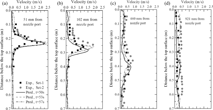
The locally predicted velocity profiles at a special time (50 s) for case A3 against the measured velocities²⁵⁾ at Inland Steel are shown in Fig. 5. The measurements of time-averaged velocity were made along a vertical line in the center plane at 5 mm from the narrow wall of the mold. The comparison suggests that the predictions agree reasonably well with the measurements, except for some small differences in magnitude. These measurements also show that the velocity on the right side of the water model is larger than that of the left side. This flow asymmetry can be accounted for in this LES model results here.

Fig. 5.

Comparison of calculated and measured velocity profiles near narrow wall in water model²⁵⁾ (Case A3 in Table 1).

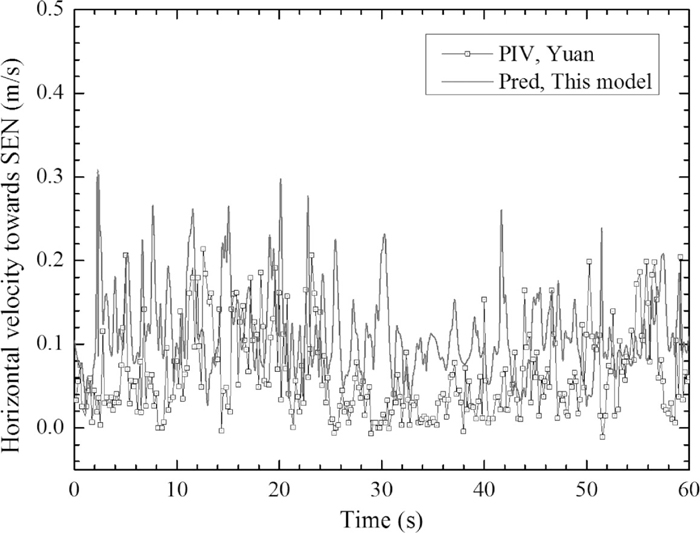
The highly turbulent fluid flow history plays an important role on flow behavior inside a continuous casting mold. A comparison of the LES model with previous measurements²²⁾ of transient horizontal velocities toward the SEN at a typical point a 0.4-scale water model for case A4 is presented in Fig. 6. This point is located at 20 mm below the top surface, midway between the SEN and narrow wall of the mold. Instantaneous velocities were collected every 0.01 seconds by the PIV for 60 seconds of data, but the sample velocity signals have 0.2 seconds temporal filtering so the higher frequencies cannot be captured. In order to match well with the variations in the measured sample velocity signals, the predictions of LES were also monitored every 0.2 seconds. Due to the instability of turbulence, the chaotic turbulent flow histories are never exactly reproducible. So it is observed that the LES model can capture the similar transient behavior with the measured signals. Overall, the LES model and calculation method established in this work is confirmed to be reliable.

Fig. 6.

Comparison of calculated and measured²²⁾ time history of horizontal velocity toward SEN at point 20 mm below the top surface (Case A4 in Table 1).

4. Results and Discussion

4.1. Instantaneous Flow Structures

The instantaneous flow structure is important, because it greatly affects the transport of harmful non-metallic inclusions inside the liquid pool. A typical instantaneous velocity field in the liquid pool obtained from the LES model is shown in Fig. 7. Molten steel escapes from the SEN port as a strong jet, diffuses as it traverses across the liquid pool, impinges on the narrow wall, and splits into two recirculation zones consisting of complex multiple vortex structures. The whole flow field is obvious asymmetry, as shown in Fig. 7(a). Comparing with the results shown in Fig. 2, the LES model can capture more details of the turbulent flow. The flow consists of a range of scales, as seen by the velocity variations within the flow field. Several large-scale vortices can be observed both in the upper roll and lower roll of the liquid pool, which suggests the dominance of large-scale structures in these regions. In addition, a lot of small-scale vortices can be observed between these large-scale vortices. Along the top surface, velocity from the right narrow wall to the SEN is larger than the left one, owing to the asymmetrical flow in the upper roll.

Fig. 7.

Predicted instantaneous velocity fields at the center plane between wide faces (a) and 10 mm below the top surface (b).

Figure 7(b) shows the flow field in the cross section of 10 mm below the top surface (meniscus). It can be seen that the flow structure is not symmetric and a big vortex is observed near the SEN on the left side of the mold, corresponding the direction of Fig. 7(a). This vortex is composed of a three-dimensional downward flow toward the outlet and a two-dimensional rotation planar vortex. It can cause the mold powder entrapment and carry the entrapped flux deeply down into the molten pool. So understanding the vortex formation is important for improving the quality of steel product. More details of vortex flow behaviors on the meniscus are presented in the next section.

4.2. Instantaneous Vorticity Fields

It is well known that the swirling flow (vortex) is found in both upper and lower roll of the continuous casting mold, which can trigger instabilities of the molten steel flow. Therefore, it is necessary to analyze the vortex distribution inside the mold. Vorticity represents the orientation and angular velocity of local rotation and therefore it is often used as a criterion for the existence of vortices, and also used to describe the creation, transformation and extinction of vortex. In order to get a better understanding of the turbulent flow inside the liquid pool, it is of interest to examine the vorticity distribution and its role in vortex phenomena.

Vorticity is a measure for the rotation of fluid element (velocity swirling strength) in the flow field, namely the curl of velocity field, is twice as the rotating speed of fluid:   

$$\mathrm{\Omega }=\nabla \times \overrightarrow{u}=2\omega$$(8)

where Ω is vorticity; $\overrightarrow{u}$ is velocity vector of molten steel, ω is the rotate angular speed of molten steel.

Figure 8 shows the vorticity field of molten steel inside the liquid pool of the thin slab mold, (a) is the iso-surface distribution of various vorticity magnitudes; (b) is the 2-D vorticity distribution in the center plane; (c) is the 2-D vorticity distribution in various cross sections and the iso-surface distribution of high intensity vorticity. Vorticity is present in any vortex and it often gives a simpler representation because of the rotational nature of vortices. Many pronounced large scale vortex structures can be clear found inside the mold, containing various small scale vortices between them. The distribution is also asymmetric, corresponding to the asymmetrical flow in the lower roll of the mold, as shown in Figs. 8(a) and 8(b).

Fig. 8.

Predicted instantaneous vorticity fields, including the iso-surface of various vorticity magnitudes (a), the 2-D vorticity in the center plane (b), and the 2-D vorticity in various cross sections and the iso-surface of high intensity vorticity (c).

However, the vorticity is presented not only in vortices but also in shear flow, and the boundary shear flow often plays an important role in the creation of vortices. As shown in Figs. 8(b) and 8(c), the highest vorticity magnitudes often can be found along the jet and near the narrow wall rather than within vortices. This can help the understanding of how boundary shear flow detaches and contributes to vortices. The shear flow can separate from the boundary, this way transporting vorticity into the interior of the flow, and possibly developing into a vortex, as shown in Fig. 8(c), at the lower roll of the mold.

4.3. Meniscus Instability

Transient flow, caused by wobbling jets, may cause intermittent chaotic vortex formation on both sides of the SEN at the meniscus. This vortex phenomenon can make the molten steel generate downward suction to involve the liquid slag into the steel pool, and deteriorate cleanness of the molten steel. Many water modeling studies have revealed that the existence of vortex in the mold is adjacent to the SEN. Therefore, it is essential to understand the behavior of vortex flow inside the mold for the design of effective methods of reducing the mold powder entrapment.

Figures 9(a) to 9(f) shows the predicted various vortex flow patterns 10 mm below the meniscus at some arbitrary times. At 89 s (Fig. 9(a)) and 134 s (Fig. 9(b)), one big vortex is located at the left side and right side of the SEN, respectively. At an arbitrary of 10 s, in Fig. 9(c), two vortices are found at the left side of the SEN. 66 s later, in Fig. 9(d), there are two vortices at the right side of the SEN. In particular, at 101 s, two vortices are located at both sides of the SEN with diagonal distribution; this is the first time to found this phenomenon in a thin slab mold using a mathematical model. Another important finding of three vortices at the meniscus are obtained using this model, as shown in Fig. 9(f), two vortices are located at both sides of the SEN with diagonal distribution, another one is located between the SEN and wide wall of the mold. All the results show that the vortexing flow in the thin slab mold is complex, and the LES model is able to capture these phenomena.

Fig. 9.

Predicted various vortex flow patterns 10 mm below the top surface at some arbitrary times (a) 89 s, (b) 134 s, (c) 10 s, (d) 76 s, (e) 101 s, and (f) 29 s.

Figure 10 shows the predicted horizontal velocities along the centerline between wide walls of 10 mm below the meniscus for these times (Fig. 9). The velocities of the two sides around the SEN are clearly different. Compared with the results of vortexing flow pattern in Fig. 9, the vortex is located at the low velocity side adjacent to the SEN. The molten steel flow from the high velocity side through the side of the SEN meets the flow from the low velocity side, and shearing takes place to form a vortex.

Fig. 10.

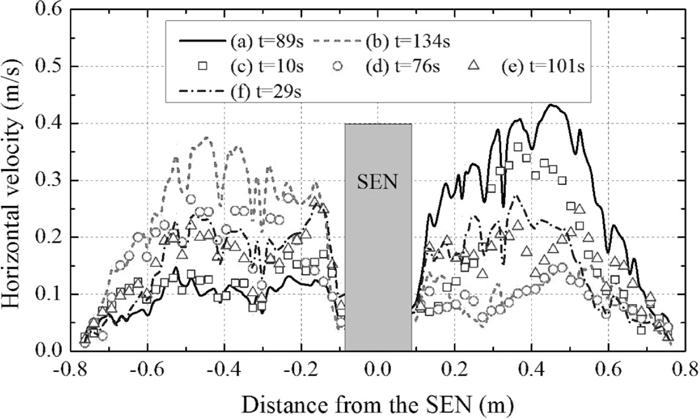
Predicted horizontal velocity along the centerline 10 mm below the meniscus at different times.

4.4. Evolution of Asymmetrical Flow Pattern

A number of workers reported that the flow pattern inside the mold is not stationary but changes over frequently. And a few people analyzed the origins of asymmetries in continuous casting mold through estimating of scales of turbulence and the balance of the turbulent kinetic energy. Different from those works, the periodical asymmetrical flow pattern inside the thin slab mold is identified and characterized in the present work. Figures 11(a) through 11(f) present the transient flow pattern inside the mold at different times. The long-term flow asymmetry in the lower recirculation zone is observed. The flow pattern is ever-changing; this result fully shows that the mold turbulent field is transient and random. And the time-averaged RANS model cannot reflect the important feature. The result further reveals the significant flow asymmetry in the lower recirculation zone, and the evolution of asymmetric flow can be divided in two processes:

Fig. 11.

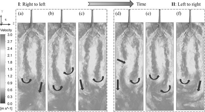
Evolution of asymmetrical flow pattern inside the mold, including two processes: left to right ((a) to (c)), and right to left ((d) to (f)).

I) Evolution of asymmetric flow from right to left: At a time of 146 seconds, the left jet turns upward at about 3.2 m below the top surface, and the right jet keep downward along the narrow wall, leading the molten steel discharge through the right half of the mold, as shown in Fig. 11(a). 3 seconds later, in Fig. 11(b), the right jet begins turn left to the center and gradually connects with the upward jet; on the contrary, the left jet separate with previous upward flow jet and gradually turn downward. At 152 seconds, in Fig. 11(c), the complete right jet turns upward at also about 3.2 m below the top surface, and the left jet keep downward along the narrow wall, leading the molten steel discharge through the left half of the mold.

II) Evolution of asymmetric flow from left to right: The changing process is similar with process I, the difference between I and II is the direction of asymmetric flow, which would changes from the left to the right, as shown in Figs. 11(d) to 11(f).

4.5. Periodicity of Asymmetrical Flow Pattern

In order to analyze the periodicity of the asymmetrical flow pattern, five points were selected, as illustrated in Figure 12. Two points are located at 10 mm below the top surface, midway from the SEN and the narrow wall, referring to left-P1 and right-P2. Another two points are located at 0.355 m below the top surface near the SEN, referring to left-P3 and right-P4, which are located inside the jet. The last point is located 3.2 m below the top surface at the center of the mold, referring to P5, which is located inside the upward jet. All the data were sampled every 0.01 seconds from the simulation results.

Fig. 12.

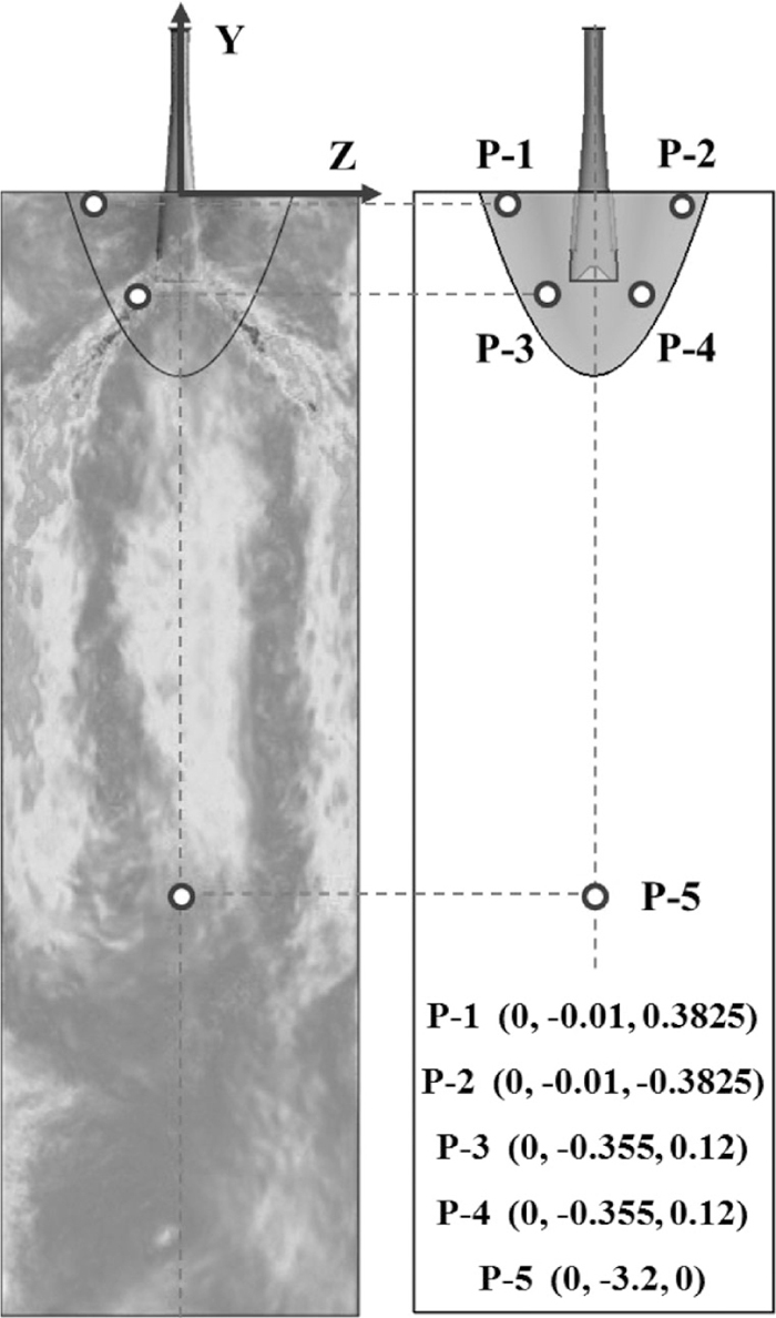
Positions of investigated points.

Figures 13(a) and 13(b) shows the model predictions of time histories of molten steel velocity at one pair of monitoring points (P3 and P4), symmetrically located in the mold (Fig. 12). The velocities are always high and variable. The plot clearly indicates that a strong high-frequency fluctuation exit in the jet escaping from the SEN port. The fluctuation frequency is about 9 to 12 Hz. The results of mean velocities show that the jets are not symmetric between sides of the SEN.

Fig. 13.

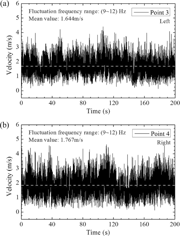
Time history of the steel velocity at points P-3 and P-4.

Figures 14(a) and 14(b) shows the time histories of molten steel velocity at another pair of monitoring points (P1 and P2), symmetrically located in the mold (Fig. 12). Compared with the result of Fig. 13, the high-frequency velocity variations decrease from the jet port to the meniscus. The fluctuation frequencies at points P1 and P2 are about 1 to 6 Hz. The results of mean velocities show that the meniscus fluctuation is not symmetric between sides of the mold.

Fig. 14.

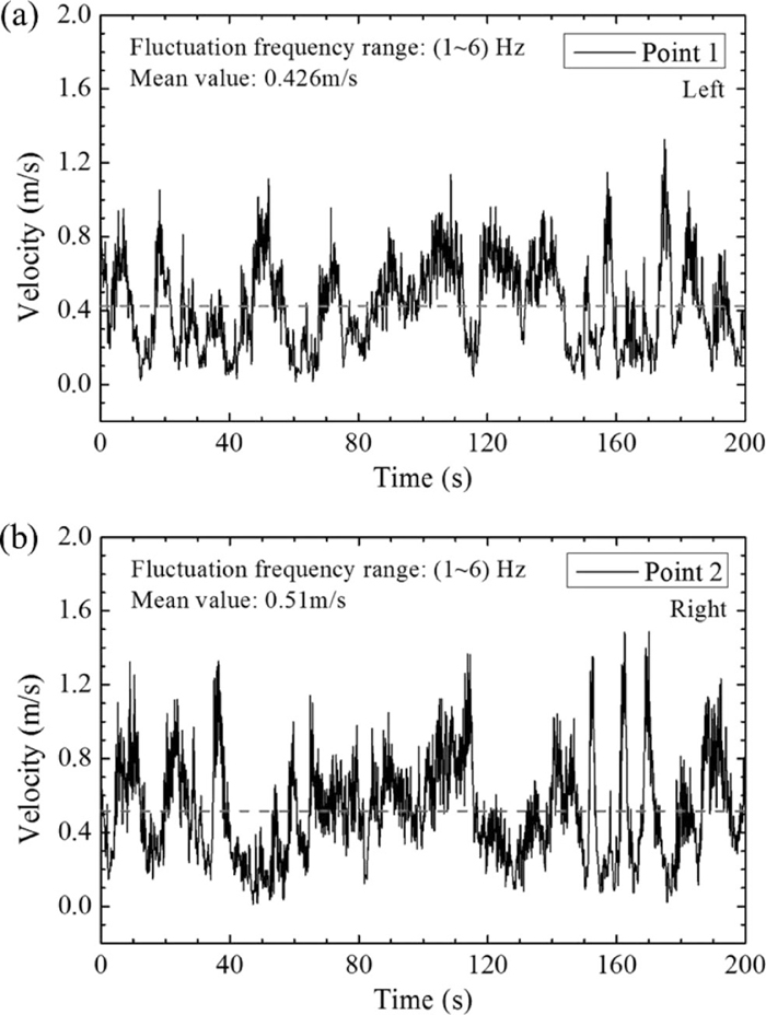
Time history of the steel velocity at points P-1 and P-2.

Figure 15 shows the model predictions of time histories of horizontal velocity (v_z) at point P5. The positive and negative value of horizontal velocity for a long time represents the recirculation flow in the lower roll turn upward from the left side and right side of the mold, respectively. The plot clearly indicates that the low-frequency long-term asymmetries exit in the lower recirculation zone. And the direction of asymmetric flow is changing with time, corresponding to the results of Fig. 11. The high-frequency velocity variations decrease from the jet port to the lower recirculation zone (1–5 Hz). The spectrum of velocities shows that the behavior of low-frequency long-term asymmetries in the lower roll was cyclical, and the mean time interval for changeover is 14.28 seconds.

Fig. 15.

Time history of the horizontal velocity at points P-5.

In order to validate the accuracy of predicted period of Fig. 15, the time histories of vertical velocities (v_y) of molten steel at point P5 is monitored, as shown in Fig. 16. Almost the values of vertical velocities are positive, indicating that the point P5 is located in the upward jet. So the prediction of Fig. 15 is effective. However, the time period of asymmetrical flow would be affected by other geometric and operating parameters, such as structure of the nozzle, casting speed, gas injection, and so on.

Fig. 16.

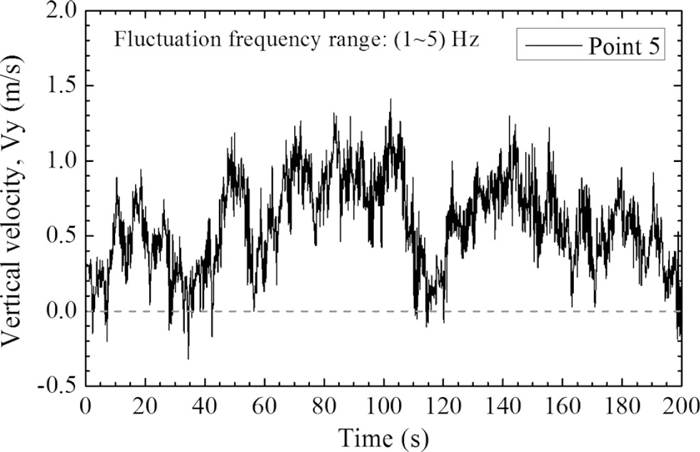
Time history of the vertical velocity at points P-5.

5. Conclusions

The instability and periodicity of the turbulence flow in a funnel thin slab continuous casting mold were studied using a transient large eddy simulation model. The predicted velocity fields were compared with previous measurements of the hot-wire anemometers and PIV. Following conclusions were obtained:

(1) The LES model can capture the similar transient behavior with the measured signals. The predicted velocities agree reasonably well with the previous measurements in the mold region. Overall, the LES model and calculation method established in this work is confirmed to be reliable.

(2) The turbulence flow consists of a range of scales vortices; many pronounced large scale vortex structures were clear found inside the mold, containing various small scale vortices between them.

(3) The vorticity is presented not only in vortices but also in shear flow, and the boundary shear flow often plays an important role in the creation of vortices. The shear flow can separate from the boundary, this way transporting vorticity into the interior of the flow, and possibly developing into a vortex.

(4) The intermittent chaotic vortex formation on both sides of the SEN was found at the meniscus. One big vortex, two vortices and three small vortices phenomena were captured using the LES model. And the vortices were located at the low velocity sides adjacent to the SEN.

(5) Significant asymmetry was seen in the instantaneous flow in the two halves of the thin slab mold cavity, especially in the lower recirculation zone. The periodical behavior of asymmetric flow inside the liquid pool was identified and characterized.

(6) The flow variations contain more energy in high frequency scales for the transient flow at the SEN ports. The high-frequency velocity variations decrease from the jet port to the meniscus and the lower recirculation zone. The spectrum of velocities shows that the behavior of low-frequency long-term asymmetries in the lower roll was cyclical, and the mean time interval for changeover is 14.28 seconds.

Acknowledgemenct

Authors are grateful to the National Natural Science Foundation of China for support of this research, Grant No. 51210007.

Nomenclature

A⁺ Constant

C_a Added mass force coefficient

C_s Smagorinsky constant

D Fluid domain

f(x) Filtered variable

g Acceleration of gravity

G(x, x′) Filter function

i, j Direction (x, y, z)

k Von Kármán constant

L Mixing length for sub-grid scales

P Pressure

S_ij Rate-of-strain tensor for the resolved scale

t Time

u Filtered velocity

V Volume of a computational cell

x, x′ Variable

y⁺ Dimensionless distance

ρ Density

μ_t Turbulent viscosity

Δ Feature length, Δ = V^1/3

τ_ij Sub-grid scale stress

v Kinematic viscosity

ω Rotate angular speed

Ω Vorticity

References

• 1)   Y.  Sahai,  J. E.  Battles. R. S. Carbonara and C. E. Mobley: Proc. Int. Symp. on Casting of Near Net Shape Products, TMS, Warrendale, PA, (1988).
• 2)   S.  Ge,  M.  Isac and  R. I. L.  Guthrie: ISIJ Int., 52 (2012), 2109.
• 3)   T.  Honeyands and  J.  Herbertson: Steel Res., 66 (1995), 287.
• 4)   H.  Nam,  H. S.  Park and  J. K.  Yoon: ISIJ Int., 40 (2000), 886.
• 5)   T. G.  Oconnor and  J. A.  Dantzig: Metall. Mater. Trans. B, 25 (1994), 443.
• 6)   Q.  Yuan,  B. G.  Thomas and  S. P.  Vanka: Metall. Mater. Trans. B, 35 (2004), 685.
• 7)   Q.  Yuan,  B. G.  Thomas and  S. P.  Vanka: Metall. Mater. Trans. B, 35 (2004), 703.
• 8)   Z. Q.  Liu,  B. K.  Li and  M. F.  Jiang: Metall. Mater. Trans. B, 45 (2014), 675.
• 9)   M. M.  Jaradeh and  T.  Carlberg: Metal. Mater. Trans. B, 43 (2012), 82.
• 10)   Z. Q.  Liu,  B. K.  Li,  M. F.  Jiang and  F.  Tsukihashi: ISIJ Int., 53 (2013), 484.
• 11)   T.  Robertson,  P.  Moore and  R. J.  Hawkins: Ironmaking Steelmaking, 13 (1986), 195.
• 12)   D.  Gupta,  S.  Subramanian and  A. K.  Lahiri: Steel Res., 62 (1991), 496.
• 13)   D.  Gupta and  A. K.  Lahiri: Metall Mater. Trans. B, 27 (1996), 757.
• 14)   B. Z.  Shen,  H. F.  Shen and  B. C.  Liu: ISIJ Int., 47 (2007), 427.
• 15)   X. H.  Wang,  X. H.  Wang,  J. M.  Zhang and  C. L.  Jing: J. University Sci. Tech. Beijing, 31 (2009), 234.
• 16)   E.  Torres-alonso,  R. D.  Morales,  S.  García-hernández and  J.  Palafox-ramos: Metall. Mater. Trans. B, 41 (2010), 583.
• 17)   B. K.  Li,  Z. Q.  Liu,  F. S.  Qi,  F.  Wang and  G. D.  Xu: Acta Metall. Sin., 48 (2012), 23.
• 18)   B. K.  Li and  F.  Tsukihashi: ISIJ Int., 46 (2006), 1833.
• 19)   H. P.  Liu,  C. Z.  Yang,  H.  Zhang,  Q. J.  Zhai and  Y.  Gan: ISIJ Int., 51 (2011), 392.
• 20)   H.  Arcos-gutierrez,  G.  Barrera-cardiel,  J. J.  Barreto and  S.  García-hernández: ISIJ Int., 54 (2014), 1304.
• 21)   E.  Torres-alonso,  R. D.  Morales and  S.  García-hernández: Metall Mater. Trans. B, 41 (2010), 675.
• 22)   Q.  Yuan,  S.  Sivaramakrishnan,  S. P.  Vanka and  B. G.  Thomas: Metall. Mater. Trans. B, 35 (2004), 967.
• 23)   A.  Ramos-Banderas,  R.  Sánchez-Pérez,  R. D.  Morales,  J.  Palafox-Ramos,  L.  Demedices-Garcia and  M.  Diaz-Cruz: Metall. Mater. Trans. B, 35 (2004), 449.
• 24)   B. G.  Thomas,  X.  Huang and  R. C.  Sussman: Metall. Mater. Trans. B, 25 (1994), 527.
• 25)   Y. H.  Wang: Proc. 75th Steelmaking Conf., The Iron and Steel Society, Warrendale, PA, (1992), 271.
• 26)   J.  Smagorinsky: Monthly Weather Rev., 91 (1963), 99.
• 27)   R.  Eriksson,  L.  Jonsson and  P. G.  Jonsson: ISIJ Int., 44 (2004), 1358.
• 28)   E. R.  Van Driest: J. Spacecraft Rockets, 40 (2003), 1012.