Numerical Modeling of Macrosegregation in Round Billet with Different Microsegregation Models

Abstract

A macrosegregation model, coupling fluid flow, heat and solute transport model, was developed based on continuum model to predict the evolution of macrosegregation in continuous round billet casting, as well as the influence of microsegregation model choice on prediction of macrosegregation. Evolution and characteristics of macrosegregation corresponding to predicted solidification were revealed. As solidification proceeds, solutes are ejected from solid phase to liquid at solidification front. The resulting mushy zone is enriched by solutes, due to the low velocity and limited diffusion, which produces segregation at the billet center as the liquid available for dilution diminishes near the end of solidification. Predicted and experimental results for surface temperature and centerline segregation compare agreeably, which indicates the validity of the coupled macrosegregation model in this work. A detailed analysis was performed to investigate the influence of microsegregation model on prediction of macrosegregation, demonstrating that choice of model affects predicted segregation degree of solutes, which effect varies with type of solute, due to the solute back-diffusion coefficient.

1. Introduction

Macrosegregation, namely compositional inhomogeneity at a scale much larger than microstructure,¹⁾ develops on whole-cast scale during solidification of multicomponent alloys. This compositional heterogeneity of cast structure results in non-uniformity of the mechanical properties of metal products, and lowers overall quality. Moreover, macrosegregation results in more serious quality problems as compared to microsegregation because macroscopic uniformity cannot be achieved by heat treatment as low diffusion coefficient in solid even at elevated temperatures. As a result, recent decades have seen some research on the formation and control of macrosegregation.

Numerical simulation has been a primary method in the study of macrosegregation since Flemings and co-workers^2,3,4) discovered that convection within the mushy zone significantly influences macrosegregation, and thus derived “local solute redistribution equation” (LSRE) to describe macrosegregation due to inter-dendritic liquid flow based on some assumptions: (i) the liquid is well mixed and in local equilibrium with the solid, and (ii) there is no diffusion in the solid. Based on LSRE, Mehrabian et al.⁵⁾ applied Darcy’s law in the calculation of the inter-dendritic flow velocities, assuming the mushy zone to be a porous medium. Based on investigations of aluminium-copper alloy ingots, a critical condition of flow was shown to lead to flow instability with resulting formation of “channel-type” segregation. In previous studies, temperature field in the mushy zone has been assumed or measured to serve as input to the analysis of the inter-dendritic convection. Fuji et al.⁶⁾ extended the macrosegregation theory to predict “channel-type” segregation of low-alloy steel. For the first time, calculation in the study combines the conservation equations of energy and momentum with LSRE and solves them simultaneously. Although encouraging results for macrosegregation had been previously obtained, reported research models ignore flow in bulk liquid regions. Given the described flaw, Ridder et al.⁷⁾ coupled fluid flow in the liquid zone to inter-dendritic flow in the mushy zone in a macrosegregation model for the first time, and then solved the coupled set of equations given by LSRE, Darcy’s law, and energy equation in mushy zone, as well as the momentum and energy equations in fully liquid region. Predicted results reported by Ridder et al.⁷⁾ for macrosegregation agree well with the experimental measurements. However, since the governing equations for fluid flow in each region are quite different, the momentum equation was written and solved separately in the cited work, but coupled through certain interfacial conditions in a multi-domain approach. The primary difficulty associated with the multi-domain model focus on tracking the phase interface, which is generally an unknown function of space and time in multicomponent alloy systems. In order to overcome the difficulty and to better incorporate solidification physics, a single-domain continuum model,^8,9) based on classical mixture theory, as well as a volume-averaged model,^10,11) have been proposed in earlier research. Favourable results have been obtained by applying the described models to quantitatively predict macrosegregation in cast alloys.^{12,13,14,15,16)}

Solute redistribution occurring at a moving solid-liquid interface, calculated by the microsegregation model, is known to play a significant role in the modeling of macrosegregation. A few microsegregation models, including the Lever rule, Gulliver-Scheil equation (Scheil), Brody-Flemings (BF) model, Ohnaka model, Clyne-Kurz (CK) model and Voller-Beckermann (VB) model, are reported in previous works. Among those listed, the Lever rule was adopted extensively for simulation of macrosegregation because of its simplicity, which model assumes the solidification system to remain in thermodynamic equilibrium, allowing for infinite solute diffusion in both liquid and solid phases. Apparently, equilibrium is not operative in the whole system throughout solidification; hence the given assumption is not appropriate to solidification of multicomponent alloys. Given that solutes diffuse slowly in solid phase, neglect of diffusion in solid is more accurate, while the solute diffusion in liquid phase is still assumed to be infinite. This non-equilibrium treatment leads to the famous Gulliver-Scheil equation.¹⁷⁾ However, solutes diffuse to a certain extent in the solid phase, and final concentration cannot be obtained by the Gulliver-Scheil equation. Attempts were therefore made to account for a finite diffusion coefficient in solid phase. Developed in the mid-1960s, the Brody-Flemings model,¹⁸⁾ introduced the Fourier number, $\alpha \text{=}{D}_s^2{t}_f/X^2$, to consider back-diffusion of solutes, and the back-diffusion coefficient was defined to be: β=2α. Brody-Flemings’ results have been reported to overestimate the amount of solid-state diffusion during solidification, especially for slow solidification, where the solute Fourier number is large. Clyne and Kurz¹⁹⁾ modified the back-diffusion coefficient, developing Clyne-Kurz model based on the Brody-Flemings model. However, the said model was criticized by Ohnaka²⁰⁾ and Matsumiya²¹⁾ for lack of physical basis for intermediate back-diffusion coefficient values of solutes. Subsequently, Ohnaka proposed two modifications of back-diffusion coefficient for solutes, which modifications more closely approximate Matsumiya’s experimental results²¹⁾ than other models. Voller and Beckermann added an additional term to the Fourier number to account for the coarsening of microstructure in their famous model,^22,23) which treatment correctly incorporates back-diffusion behavior with solute redistribution for both small and large Fourier numbers.

For continuous casting, little research^24,25) is reported on the prediction of macrosegregation in strands and the influence of microsegregation models on this aspect remains enigmatic. Moreover, almost entirely previous simulations of macrosegregation were performed based on the lever rule microsegregation model, which is inadequate for the solidification of steel. The main purpose of this paper is to reveal the evolution of macrosegregation during continuous round billet casting with a macrosegregation model, in which different microsegregation models are coupled to uncover the influence of microsegregation models on distribution of solutes.

2. Model Description

2.1. Assumptions

In Fig. 1 appears the schematic representation of a continuous round billet caster, and the main technical parameters are listed in Table 1. In practice, the molten steel is continuously poured into the mold through a submerged entry nozzle and the strand is drawn away at a constant casting speed. This macrosegregation model was developed based on the following assumptions:

Fig. 1.

Schematic representation of continuous round billet caster. (Online version in color.)

Table 1. Main technical parameters of the caster.

Parameters	Values
Mould length	0.8 m
Machine type	Curved
Machine radius	10 m
Casting speed	1.65 m/min
Inner diameter of SEN	0.035 m
Outer diameter of SEN	0.075 m
Immersion depth of SEN	0.1 m

(a) The molten steel was assumed to be incompressible and turbulence effects were approximated with the Low-Reynolds number model.

(b) Given the symmetry of round billet and the sake of computational cost, a two-dimensional simulation was adopted in this work, although this assumption may not essentially a good approximation.

(c) Local thermodynamic equilibrium during solidification was assumed to prevail at solid-liquid interface.

(d) The effects of deformation caused by bulging on solute distribution and fluid flow were considered to be negligible.

(e) Only the vertical part of the caster was considered in the simulation, and the billet curvature due to bending was ignored.

(f) The interactions between different alloying elements were ignored.

2.2. Fluid Flow

The governing equations describing the fluid flow during continuous casting take the following form:   

$$\frac{\partial \rho }{\partial t}+\nabla \cdot \left(\rho \overrightarrow{u}\right)=0$$(1)

where ρ is density, t is time and $\overrightarrow{u}$ is velocity.   

$$\begin{array}{l}\frac{\partial \left(\rho \overrightarrow{u}\right)}{\partial t}+\nabla \cdot \left(\rho \overrightarrow{u}\overrightarrow{u}\right)\\ =\nabla \cdot \left({\mu }_{eff}\nabla \overrightarrow{u}\right)-\nabla p+\rho \overrightarrow{g}-\nabla \cdot \left[\rho f_s\left(\overrightarrow{u}-{\overrightarrow{u}}_s\right)\left({\overrightarrow{u}}_l-{\overrightarrow{u}}_s\right)\right]-S_u\end{array}$$(2)

with ${\overrightarrow{u}}_s$ and ${\overrightarrow{u}}_l$ being the velocity of solid and liquid, p the pressure, μ_eff the effective viscosity, and f_s, f_l the corresponding fractions. The source term S_u can be described as following equation:   

$$\begin{array}{l}{S}_u=\rho \overrightarrow{g}\left[{\beta }_T\left(T-T_{ref}\right)+{\beta }_{C,i}\left(C_{l,i}-C_{\mathrm{r}\mathrm{e}\mathrm{f},i}\right)\right]\\ \hspace{1em}\hspace{0.5em}\text{+}\frac{{\left(1-f_l\right)}^2}{f_l{}^3+\xi }{A}_m\left(\overrightarrow{u}-{\overrightarrow{u}}_s\right)\end{array}$$(3)

where β_T and β_C,i represent the thermal and solutal expansion coefficient, T is temperature and C_i is concentration of element i, the subscript R identify the reference value, ξ is a very small positive number.

The first term on the right-hand side of Eq. (3) represents thermal and solutal buoyancy, which are influenced by temperature gradient and concentration gradient during solidification. Both buoyancy terms are calculated using the Boussinesq approximation. In lower part of strand, thermal buoyancy force becomes dominant in the mushy zone and plays an important role in transport phenomena, as clearly indicated by modified Froude number.²⁵⁾ The second term accounts for momentum sink due to reduced porosity in the mushy zone. With the enthalpy-porosity technique, the mushy zone is treated as a porous medium, which can be described by Darcy’s law. The porosity in each volume element is assigned equal to the liquid fraction; hence, porosity is equal to 1 in liquid and 0 in solid zones, while momentum decreases in the mushy zone along with the porosity. In Eq. (3), the permeability coefficient, A_m, depends on the porous medium morphology. In this work, A_m is calculated following Minakawa:²⁶⁾ $A_m=180/{\lambda }_2^2$, where λ₂ represents the secondary arm space and the expression used here²⁷⁾ is presented in the solute redistribution section.

The fluid flow in the upper part of mold is normally turbulent, which will affect the flow patterns, energy and solute transport. Thus, effective viscosity (μ_eff) is applied in the simulation, which is defined as the sum of laminar (μ) and turbulent viscosity (μ_t). Turbulent viscosity is calculated using the following equation:   

$${\mu }_t=\rho f_{\mu }{C}_{\mu }\frac{k^2}{\epsilon }$$(4)

where k and ε, the turbulent kinetic energy and its rate of dissipation, are calculated based on turbulent model. The low-Reynolds number k−ε model^24,28) applied here is considered to be preferable than standard two-equation k−ε model or high-Reynolds number k−ε model in continuous casting. Governing equations of the model can be written as follows:   

$$\nabla \cdot \left(\rho \overrightarrow{u}k\right)=\nabla \cdot \left[\left(\mu +\frac{{\mu }_t}{{\sigma }_k}\right)\nabla k\right]+G_k-\rho \epsilon +\rho D+S_k$$(5)

  

$$\begin{array}{l}\nabla \cdot \left(\rho \overrightarrow{u}\epsilon \right)=\nabla \cdot \left[\left(\mu +\frac{{\mu }_t}{{\sigma }_{\epsilon }}\right)\nabla \epsilon \right]+C_1{f}_1{G}_k\rho \frac{\epsilon }{k}\\ \hspace{1em}\hspace{1em}\hspace{1em}\hspace{1em}\hspace{0.17em}-C_2{f}_2\rho \frac{{\epsilon }^2}{k}+\rho E+S_{\epsilon }\end{array}$$(6)

with S_k and S_ε being the source terms for the k and ε equations, which are related to solidification as $S_k=\frac{1-f_l^2}{f_l^3+\xi }{A}_{m}k$ and $S_{\epsilon }=\frac{1-f_l^2}{f_l^3+\xi }{A}_m\epsilon$.

The coefficients and empirical constants used for the low-Reynolds number model of Launder and Sharma are listed in Table 2.

Table 2. Coefficients and empirical constants used for the low-Reynolds number model.

Parameters	Values	Parameters	Values
Gk	${\mu }_t\left(\frac{\partial u_i}{\partial x_j}+\frac{\partial u_j}{\partial x_i}\right)\frac{\partial u_i}{\partial x_j}$	D	$2\mu {\left(\frac{\partial (\sqrt{k})}{\partial x_i}\right)}^2$
E	$2\frac{\mu {\mu }_t}{\rho }{\left(\frac{{\partial }^2{u}_i}{\partial x_i\partial x_j}\right)}^2$	fμ	$exp\left[-3.4/{\left(1+\frac{{Re}_t}{50}\right)}^2\right]$
Cμ	0.09	C2	1.92
f1	1.0	σk	1.0
f2	$1-0.3exp\left(-{Re}_t^2\right)$	σε	1.3
C1	1.44	Ret	ρk2/με
Prt	0.9	Sct	1.0

2.3. Heat Transfer

To predict the temperature field and solidification behavior in continuous casting steel, energy conservation equation is given as:   

$$\frac{\partial \left(\rho H\right)}{\partial t}+\nabla \cdot \left(\rho \overrightarrow{u}H\right)=\nabla \cdot \left(k_{T,eff}\nabla T\right)$$(7)

The enthalpy H in the energy conversation equation can be described as a function of temperature:   

$$H=H_{ref}+\underset{T_{ref}}{\overset{T}{\int }}{c}_{ps}dT+f_{l}L$$(8)

with L being the latent heat of fusion, c_ps the specific heat of solid, h_ref the enthalpy at the reference temperature T_ref and the liquid fraction f_l can be calculated by:   

$$f_l=\{\begin{array}{ll}1,\hfill & T\ge T_l\hfill \\ \frac{T-T_s}{T_l-T_s},\hfill & T_s<T<T_l\hfill \\ 0,\hfill & T\le T_s\hfill \end{array}$$(9)

with T_l and T_s being the liquidus and solidus temperature respectively, which can be described as following equations:   

$$T_l=T_f+\sum m_i\cdot C_i$$(10)

  

$$T_s=T_f+\sum m_i\cdot C_i/k_{p,i}$$(11)

with T_f being the fusion temperature of pure iron, m_i the slope of liquidus line and k_p,i the equilibrium partition coefficient of element i.

Considering the influence of turbulence, heat conductivity is represented by the effective thermal conductivity k_T,eff:²⁹⁾   

$$k_{T,eff}=\{\begin{array}{l}\mathrm{\hspace{0.17em} }{k}_{T,l}+\frac{{\mu }_t}{{Pr}_{\mathrm{t}}},\mathrm{\hspace{0.17em} }\mathrm{\hspace{0.17em} }\mathrm{\hspace{0.17em} }\mathrm{\hspace{0.17em} }\mathrm{\hspace{0.17em} }\mathrm{\hspace{0.17em} }\mathrm{\hspace{0.17em} }\mathrm{\hspace{0.17em} }\mathrm{\hspace{0.17em} }\mathrm{\hspace{0.17em} }T\ge T_l\\ k_{T,s}{f}_s+k_{T,l}{f}_l,\mathrm{\hspace{0.17em} }\mathrm{\hspace{0.17em} }\mathrm{\hspace{0.17em} }\mathrm{\hspace{0.17em} }\mathrm{\hspace{0.17em} }{T}_s<T<T_l\\ \mathrm{\hspace{0.17em} }{k}_{T,s},\mathrm{\hspace{0.17em} }\mathrm{\hspace{0.17em} }\mathrm{\hspace{0.17em} }\mathrm{\hspace{0.17em} }\mathrm{\hspace{0.17em} }\mathrm{\hspace{0.17em} }\mathrm{\hspace{0.17em} }\mathrm{\hspace{0.17em} }\mathrm{\hspace{0.17em} }\mathrm{\hspace{0.17em} }\mathrm{\hspace{0.17em} }\mathrm{\hspace{0.17em} }\mathrm{\hspace{0.17em} }\mathrm{\hspace{0.17em} }\mathrm{\hspace{0.17em} }\mathrm{\hspace{0.17em} }\mathrm{\hspace{0.17em} }T\le T_s\end{array}$$(12)

The turbulent Prandtl number Pr_t is listed in Table 2.

2.4. Solute Transport and Redistribution

The solute transport behavior in continuous casting can be calculated by the species conservation equation:   

$$\begin{array}{l}\frac{\partial \left(\rho C_i\right)}{\partial t}+\nabla \cdot \left(\rho \overrightarrow{u}{C}_i\right)=\nabla \cdot \left(\rho f_s{D}_{s,i}\nabla C_{s,i}\right)\\ +\nabla \cdot \left(f_l\left(\rho D_{l,i}+\frac{{\mu }_t}{S{c}_t}\right)\nabla C_{l,i}\right)\\ -\nabla \cdot \left[\rho f_s\left(\overrightarrow{u}-{\overrightarrow{u}}_s\right)\left(C_{l,i}-C_{s,i}\right)\right]\end{array}$$(13)

where D_s,i and D_l,i are the solute diffusion coefficient in solid and liquid respectively. The turbulent Schmidt number Sc_t is listed in Table 2, and solid velocity ${\overrightarrow{u}}_s$ is equal to casting speed. The last term of Eq. (13) represents the source term induced by convection. The mixture velocity and species concentration are defined as follows:   

$$\overrightarrow{u}=f_s{\overrightarrow{u}}_s+f_l{\overrightarrow{u}}_l$$(14)

  

$$C_i=f_s{C}_{s,i}+f_l{C}_{l,i}$$(15)

As reported previously, macrosegregation results essentially from microsegregation and the relative movement between solid and liquid phases. Thus, predicting solute redistribution at solidification front is very important in macrosegregation modeling and several microsegregation models: the Lever rule, Gulliver-Scheil equation, Brody-Flemings model, Ohnaka model, Clyne-Kurz model and Voller-Beckermann model have been developed.

2.4.1. Lever Rule

Assuming the solidification system remains in thermodynamic equilibrium, which implies infinite solute diffusion in both solid and liquid phases, solute redistribution during solidification can be described as follows:   

$$C_{l,i}=C_{l,i}^{*}=C_i{[1-(1-k_{p,i})\cdot f_s]}^{-1}$$(16)

  

$$C_{\mathrm{s},i}=C_{\mathrm{s},i}^{*}=k_{p,i}{C}_i{[1-(1-k_{p,i})\cdot f_s]}^{-1}$$(17)

with C_l,i and C_s,i being the concentration of solute element i in liquid and solid, respectively, superscript * refers to the values at solid-liquid interface.

2.4.2. Gulliver-Scheil Equation

Solute diffusivity in solids, even at temperatures as high as solidus, remains orders-of-magnitude smaller than in liquid. Thus, solute diffusion in the solid phase is ignored, while complete diffusion is still assumed in the liquid, as follows:   

$$C_{l,i}=C_{l,i}^{*}=C_i{\left(1-f_s\right)}^{k_{p,i}-1}$$(18)

Local thermodynamic equilibrium is assumed to exist only at the solid-liquid interface, thus, the solute concentration in solids does not equal that at the interface.   

$$C_{\mathrm{s},i}\ne C_{\mathrm{s},i}^{*}=k_{p,i}{C}_i{\left(1-f_s\right)}^{k_{p,i}-1}$$(19)

2.4.3. Brody-Flemings Model

Accounting for the effect of back-diffusion through the solidified solid, Brody and Flemings modified the Gulliver-Scheil equation by introducing the solute Fourier number, α_i, and solute back-diffusion coefficient, β_i.   

$${\alpha }_i=\frac{D_{s,i}\cdot t_f}{X^2}=\frac{4D_{s,i}\cdot t_f}{{\lambda }_2^2}$$(20)

  

$${\beta }_i=2{\alpha }_i$$(21)

  

$$C_{l,i}=C_{l,i}^{*}=C_i{\left(1-\left(1-{\beta }_i{k}_{p,i}\right)\cdot f_s\right)}^{\left(k_{p,i}-1\right)/\left(1-{\beta }_i{k}_{p,i}\right)}$$(22)

where t_f is local solidification time, X is the microsegregation domain length at end of solidification, usually assumed to equal to half the final secondary dendrite arm spacing, λ₂.

Large solute Fourier numbers appear during slow solidification, which effect leads to overestimation of back-diffusion in solid phase. To overcome limitations of the Brody-Flemings model, some scholars developed models modifying the solute back-diffusion coefficient.

(a) Clyne-Kurz model:   

$${\beta }_i=2{\alpha }_i\left(1-exp\left(-\frac{1}{{\alpha }_i}\right)\right)-exp\left(-\frac{1}{2{\alpha }_i}\right)$$(23)

(b) Ohnaka model:

${\beta }_i=\frac{4{\alpha }_i}{1+4{\alpha }_i}$ or $\frac{2{\alpha }_i}{1+2{\alpha }_i}$ for the columnar or plate models.

(c) Voller-Beckermann model:   

$${\beta }_i=2{\alpha }_i{}^{+}\left(1-exp\left(-\frac{1}{{\alpha }_i{}^{+}}\right)\right)-exp\left(-\frac{1}{2{\alpha }_i{}^{+}}\right)$$(24)

  

$${\alpha }_i^{+}={\alpha }_i+{\alpha }^C$$(25)

where α^C is the additional term of Fourier number, whose value was determined as 0.1 by Voller and Beckermann.^22,23)

In the present study, the final secondary dendrite arm spacing, which varies with cooling conditions and alloy composition, was calculated using empirical equations proposed by Won and Thomas.²⁷⁾   

$${\lambda }_2(\mu m)=\{\begin{array}{l}(169.1-720.9\cdot C_C)\cdot C_R^{-0.4935},0<{\mathrm{C}}_{\mathrm{C}}<0.15\\ 143.9\cdot C_C^{(0.5501-1.996\cdot C_C)}\cdot C_R^{-0.3616},{\mathrm{C}}_{\mathrm{C}}>0.15\end{array}$$(26)

with C_R being the cooling rate and C_C the carbon content.

The liquidus and solidus lines in phase diagram are still assumed to be straight, meaning that the partition coefficient, k_p,i, is a constant. Thus, solute redistribution at the solid-liquid interface can be described as follows:   

$$C_{s,i}^{*}=k_{p,i}{C}_{l,i}^{*}$$(27)

For the above microsegregation models, solute concentration in liquid phase is equal to that at the solid-liquid interface, due to the assumption of complete diffusion in liquids. However, situation is different in solid phase; the solute concentration in the solid cannot be represented by the interfacial concentration, except in the case of the Lever rule (complete diffusion is also assumed in the solid). To obtain the solute concentration in solid phase, Schneider and Beckermann³⁰⁾ assumed a microscopically well-mixed solid during solidification under the Scheil model, which is similar to the Lever rule in that the solid concentration remains constant. Another treatment³¹⁾ integrating interfacial solid composition profiles has been reported for calculation of solid concentration. In this work, the following equation was derived to calculate the solid concentration:   

$$C_{s,i}=\left(C_i-f_l\cdot \frac{C_{s,i}^{*}}{k}\right)/\left(f_s+\xi \right)$$(28)

3. Computational Procedure

3.1. Numerical Method

In this work, the coupled model was solved using the open-source software OpenFOAM. The finite volume method (FVM) applies here to the set of macroscopic transport equations, giving temperature and concentration fields as input parameters for the microsegregation model. Next, dendritic structure, liquid fraction and solute distribution at the solidification front calculated by the microsegregation model were reapplied to the macrosegregation model to update values for flow, temperature and concentration fields. The large time-step transient solver, PIMPLE (merged PISO-SIMPLE) algorithm, was used in solving the pressure-velocity coupling, which algorithm demonstrates superior numerical stability in large time-steps calculations as compared to PISO. The Pressure Implicit Splitting Operator (PISO) algorithm³²⁾ is applied in the PIMPLE algorithm to rectify the pressure-velocity correction, while the Semi-Implicit Method for Pressure-Linked equations (SIMPLE) algorithm allows calculation of pressure from velocity components on a mesh by coupling Navier-Stokes equations with an iterative procedure. Thus, both numerical stability and efficiency can be achieved through the PIMPLE algorithm. About 5 hours are required to perform a fully-coupled simulation of a 0.165*10 m round billet with 37720 grid cells on a workstation with 3.4 GHz CPU and 16 GB RAM in parallel.

3.2. Boundary Conditions

The boundary conditions considered applicable to the simulation of macrosegregation in continuously cast round billet are described as follows:

3.2.1. Meniscus

Considering the insulating effect of mold flux, the free surface was set to be adiabatic wall. And the normal gradients of other variables were set to be zero.

3.2.2. Inlet and Outlet

Molten steel is introduced to the mold through a straight nozzle at a certain flow rate corresponding to the casting speed. The inlet velocity profile was assumed to be flat and determined based on the inlet-outlet mass balance. Thus, boundary conditions of all variables at the inlet can be described as follows:   

$$u_x=0,u_y=0,u_z=u_{in}=\frac{\pi d_{in}^2}{4d_s^2}{u}_c$$(29)

  

$$k_{in}=0.01u_{in}^2,{\epsilon }_{in}=k_{in}^{1.5}/R_{noz}$$(30)

  

$$T_{in}=T_c,C_{in,i}=C_{0,i}$$(31)

Turbulent kinetic energy and its rate of dissipation were calculated using the semi-empirical equations proposed by Lai et al.³³⁾ At outlet, fully developed condition was adopted for the fluid flow, and normal gradients of all variables were set to be zero.

3.2.3. Moving Wall

Velocity of the moving wall (strand surface) was set to equal casting speed, and the detailed thermal boundary conditions are given as follows:

(a) Mold zone:   

$$q_m=2\mathrm{\hspace{0.17em} }680\mathrm{\hspace{0.17em} }000-b\sqrt{L_z/u_c}$$(32)

where b is an unknown coefficient:   

$$b=\frac{1.5\times (2\mathrm{\hspace{0.17em} }680\mathrm{\hspace{0.17em} }000-\overline{q})}{\sqrt{L_m/u_c}}$$(33)

where q is the average heat flux at mold surface:   

$$\overline{q}=\frac{C_W\times Q_W\times \mathrm{\Delta }T}{S_{eff}}$$(34)

where C_W is the specific heat of water, Q_W is the flow rate of cooling water, ΔT is the temperature difference of cooling water and S_eff is effective area of mold.

(b) Secondary cooling zone:   

$$q_s=h(T_{surf}-T_W)$$(35)

where T_surf is the surface temperature of billet, T_W is the temperature of cooling water, and h is the integrative heat transfer coefficient, which can be calculated using the following equations:

Foot-roller zone:³⁴⁾   

$$h=1\mathrm{\hspace{0.17em} }570Q_W^{0.55}\left(1-0.0075\left(T_W-273.15\right)\right)/4$$(36)

Other spray zones:³⁵⁾   

$$h=116+10.44Q_W^{0.851}$$(37)

(c) Air cooling zone:   

$$q_a=\sigma e(T_{surf}+T_{ambi})\left(T_{surf}^2+T_{ambi}^2\right)$$(38)

where σ is Stefan-Boltzmann constant, ε is blackness at billet surface and T_ambi is ambient temperature, and the flow rates of cooling water Q_W in secondary cooling zone are shown in Table 3.

Table 3. Flow rate of cooling water and length of each cooling zone in secondary cooling zone.

Zone number	Zone 0	Zone 1	Zone 2	Zone 3
Flow rate of cooling water (ℓ/min)	65.24	70.88	37.48	24.77
Length of cooling zone (m)	0.304	2.450	2.401	1.502

3.3. Technological and Thermophysical Parameters

High carbon steel SWRH82B for wire rod application was applied in the simulation. Chemical compositions are listed in Table 4. Meanwhile, slope of liquidus line, equilibrium partition coefficient, solutal expansion coefficient and solute diffusion coefficient for different solute elements are also listed in Table 4. Thermophysical properties of the steel calculated with the JmatPro are listed in Table 5.

Table 4. Equilibrium partition coefficients and diffusion coefficients of different elements.

Element	C0,i (mass%)	mi (–)	kp,i (–)	βC,i36) (1/mass%)	Ds,i37) (cm2/s)	Dl,i37) (cm2/s)
C	0.81	−78.0	0.34	0.0110	0.0761exp(−134557.44/RT)	0.0052exp(−11700/RT)
Si	0.19	−7.6	0.52	0.0119	0.3exp(−251458.4/RT)	0.000514exp(−9150/RT)
Mn	0.8	−4.9	0.78	0.0019	0.055exp(−249366.4/RT)	0.00318exp(−16600/RT)
P	0.015	−34.4	0.13	0.0115	0.01exp(−182840.8/RT)	0.0135exp(−23700/RT)
S	0.008	−38.0	0.035	0.0123	2.4exp(−223425.6/RT)	0.00049exp(−8600/RT)

Table 5. Operation parameters and Thermophysical properties.

Parameters	Values
Casting speed	1.65 m/min
Pouring temperature (Tc)	1758 K
Electromagnetic stirring	No
Density (ρs = ρl = ρ)	7340 kg/m3
Solid specific heat (cp,s)	650 J/kg·K
Liquid thermal conductivity (kT,l)	33.5 W/m·K
Solid thermal conductivity (kT,s)	24.7 W/m·K
Thermal expansion coefficient (βT)	2.0×10−4 K−1
Liquid viscosity (μ)	0.00461 Pa·s
Latent heat (L)	231637 J/kg
Fusion temperature of pure iron (Tf)	1808 K

4. Results and Discussion

To investigate the evolution of macrosegregation in round billets and validate predicted results of the coupling model in this work, results of solute distribution calculated by the Lever rule will be presented and discussed first.

4.1. Fluid Flow and Solidification

Figure 2 presents the predicted distribution of velocity for the molten steel in mold, (a) the velocity profiles at billet center along casting direction, (b) the velocity contour and streamline in mold. It is observed that the molten steel is poured into the mold through a submerged nozzle, under which a high-speed flow zone forms. After that, the velocity decreases rapidly to be nearly equal the casting speed at about 0.6 m below the meniscus. And then, no evident fluctuation happens for the melt velocity in billet, and the molten steel and solidification shell come into a relatively static status. In mold, most of the molten steel flows downward into the secondary cooling zone along the caster, while a minimum of molten steel moves upward along the billet wall. Consequently, a pair of large recirculation zones are created by the impinging jet pouring from the nozzle, as shown in Fig. 2(b). A melt backflow develops at the upper region of the caster due to the mass and momentum entrainment, and the backflow region is shown in the vicinity of the initial solidification shell, wherein the velocity is equal to the casting speed.

Fig. 2.

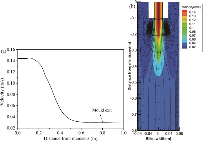
Distribution of the melt velocity in mold, (a) at centerline, (b) velocity contour. (Online version in color.)

Figure 3(a) shows the contour of the liquid fraction, which indicates the solidification process of a continuously cast round billet. The position of the crater end, shape of the mushy zone and the related solidified shell can be clearly identified in the figure. Center temperature in the round billet decreases slowly during early solidification. Correspondingly, the central liquid fraction remained at 1 up to 6.3 m from meniscus, while the billet solidified completely about 9.3 m from meniscus, which indicates about 3 m mushy zone length under studied casting conditions. Affected by decrease in evolved latent heat, the cooling rate in the mushy zone increases dramatically, this arises from change in the central liquid fraction. However, the temperature at billet surface changes slightly, as shown in Fig. 4, which is attributed to release of latent heat and weak cooling. Thermal contraction of the solidified shell reported by Raihle and Fredriksson³⁸⁾ appears late in the solidification and influences centerline segregation. However, the focus of this research is evolution of macrosegregation and influence of different microsegregation models on prediction of segregation. Thus, the effect of thermal contraction is ignored. Also shown in Fig. 3 are distributions of solute carbon and phosphorus in the billet, for convenient comparison with the liquid fraction contour, as detailed in the next section.

Fig. 3.

Contour of liquid fraction and solute concentration, (a) liquid fraction, (b) distribution of carbon, (c) distribution of phosphorus. (Online version in color.)

Fig. 4.

Calculated surface temperature and central liquid fraction. (Online version in color.)

Figure 4 details calculated surface temperature and central liquid fraction profiles as a function of distance from meniscus. Due to high cooling intensity in the mold, the temperature at billet surface sharply drops to 1210 K at the mold exit. Affected by the decline of cooling intensity and the release of latent heat, the surface temperature subsequently rises at the secondary cooling zone. The maximum surface temperature, which larger than the temperature at mold exit about 80 K, arises at zone 1. Surface temperature then decreases gradually in other secondary cooling zones and the air-cooling zone. As vast quantities of latent heat are released from the central portion of billet, the surface temperature changes very slightly up to the crater end, where the temperature is higher even than at the mold exit. The central liquid fraction, which remains 1 up to 6.3 m from meniscus, decreases rapidly at the beginning of the mushy zone. However, the solidification rate slows slightly near the crater end; this is attributed to centerline segregation, which reduces solidus temperature during solidification.

To test the model, surface temperatures measured with pyrometers were compared with calculated values obtained by the model. In practice, four infrared thermometers were placed at the 2nd and 3rd zone exits of the second cooling zone and at two positions in the air-cooling zone, which measured temperatures also appear in Fig. 4. In the figure, reasonably good agreement between simulation and experiment is readily apparent.

4.2. Evolution of Macrosegregation

The predicted distribution of solute carbon and phosphorus in round billet is shown in Figs. 3(b) and 3(c) corresponding to the liquid fraction contour. The basic cause of segregation is that the solid rejects solute elements during solidification because of reduced solubility in solids compared to liquids. Hence, as solidification proceeds, solutes are rejected from solid into liquid phase at the solidification front, while the liquid ahead of the solidification front is enriched by solute elements. Therefore, some relationships can be found in Fig. 3 for the distribution of solute elements and liquid fraction. Comparing Figs. 3(b) and 3(c) with Fig. 3(a), the concentration of solutes is relatively low in the solid region, except that at the end of solidification. For the reason that the rejected solute is redistributed, while being mixed by convection and diffusion in the liquid region, distribution of solutes in the bulk liquid is relatively more uniform than other regions. Due to low velocity and limited diffusion capacity, solute elements concentrate in the mushy zone, eventually leading to segregation at billet center under decreasing liquid for dilution. Simulation shows a very great concentration of solutes just below the limit of bulk liquid, as shown in Fig. 3(a). Despite different initial concentrations for solute carbon and phosphorus, distributions of the two elements in the billet are very similar, true also for solute Mn, Si, and S, which are not illustrated here. The preceding phenomena are considered results of equilibrium partition coefficients less than unity and extremely low solute diffusion coefficients. Thus, this report concentrates on carbon distribution to reveal solute segregation in billets even when the level of segregation varies among solute elements.

Figure 5 illustrates the segregation degree profiles of carbon across billet section at varying distances from meniscus. The segregation degree is commonly defined as: r=c/c_in, where c represents local concentration of the solute element, and c_in is the initial concentration of the solute. Results given above clearly demonstrate that segregation develops in the billet as the distance from meniscus increases. As shown in Fig. 3(a), the solidification front evolves from billet surface to center as solidification proceeds. In the process, solutes are rejected from solid into liquid phase, which is controlled by the microsegregation model. Thus, positive segregation exists in the liquid ahead of the solidification front, while segregation in the solid behind solidification front is negative, as shown in Fig. 5.

Fig. 5.

Segregation degree profiles of carbon across the billet section with different. (Online version in color.)

Centerline segregation forms completely at Y=9.6 m, where complete solidification is obtained, while predicted segregation degree of carbon is given in the figure with positive segregation (concentration peak above initial concentration) at billet center and negative segregation (concentration less than initial) on both sides. And the characteristic of centerline segregation phenomenon has been previously reported by Ghosh.³⁹⁾ As reported previously, centerline segregation reflects from the equilibrium partition coefficient, which, in turn, is dependent on equilibrium phase diagram for varied content of solutes. Smaller equilibrium partition coefficient indicates higher degree of segregation in the billet. The segregation degree of carbon at billet center is predicted to be about 1.147 for 0.81 pct C steel, while value for phosphorus is expected to be greater.

In reference to billet center, calculated liquid fraction profiles and segregation degree of carbon as a function of the distance from meniscus appear in Fig. 6(a), while the Fig. 6(b) illustrates the relationship between solidus temperature and degree of carbon segregation. Early in the solidification process, the degree of carbon segregation increases slightly as liquid remains at billet center. As solidification proceeds, the central liquid fraction reduces from 1 to 0 at the region ranging from 6.2 m to 9.3 m below meniscus, and segregation degree correspondingly increases from 1.015 to 1.147 until a plateau is reached while solidification completes. Predicted results show heavy centerline segregation at the end of solidification. As shown in Fig. 6(a) by the short dashed line, carbon segregation has basically taken shape when the value of central liquid fraction reaches 0.3. According to consensus, performing the final electromagnetic stirring (F-EMS) or mechanical soft reduction at the region corresponding to high central solid fraction does not effectively improve centerline segregation,^40,41) for which the formation of segregation is also an important cause, apart from poor fluidity. The degree of carbon segregation at billet center increases from 1.0 to 1.147 along the casting direction, which leads to decrease of solidus temperature from 1623 K to 1596 K, as shown in Fig. 6(b). The decrease in solidus temperature may result in remelting of some regions enriched by solutes.

Fig. 6.

Relationship between degree of carbon segregation and solidification parameters, (a) Central liquid fraction, (b) Solidus temperature. (Online version in color.)

4.3. Validation for the Macrosegregation

In order to validate the macrosegregation model, industrial trials were performed with the conditions listed in Tables 2 and 4. Concentration of carbon across the experimental billet section was analyzed using a carbon-sulfur analyzer. Specimens for chemical analysis were extracted using a planer at various distances from the surface of billet, and the detailed locations of the specimens at the billet section are illustrated in Fig. 7. In this work, dimension of the specimen is 2 mm in width and 10 mm in length, and the distance between each specimen is 5 mm.

Fig. 7.

Detailed locations of specimens in the experimental billet section. (Online version in color.)

The measured segregation degrees for carbon are shown in Fig. 8 and compared with predicted results. Comparisons between the predicted and experimental centerline segregation show reasonable agreement, which indicate that the coupled macrosegregation model in this work is valid. The predicted degrees of solute carbon at the billet center are lower than the measured values, which result is likely due to influence of solidification shrinkage and bridging and are neglected in the macrosegregation model. Apart from the billet center, positive segregation also exists at the billet quarter, which can be observed from the experimental results given in Fig. 8. Quartered segregation can be ascribed to columnar to equiaxed transition (CET) during solidification, which is reported in the works of Choudhary⁴²⁾ and Aboutalebi.²⁴⁾ During the growth of columnar crystals, liquid ahead of the columnar front is enriched by solutes. Reduction in temperature gradient leads CET as solidification proceeds. However, as the growth of equiaxed crystals is non-directional, the growing crystals hamper flow and diffusion of enriched liquid; hence some enriched liquid ahead of the columnar region is restricted to inter-dendritic spaces, wherein positive segregation occurs.

Fig. 8.

Comparison between calculated and measured degree of segregation for carbon. (Online version in color.)

4.4. Influence of Microsegregation Model

To evaluate the influence of microsegregation model on the solutes distribution in continuously cast billet, results of six cases are examined here. Calculations were conducted with the same casting conditions and macro-scale model, but under six different microsegregation models: the Level rule, Gulliver-Scheil model, Brody-Flemings model, Clyne-Kurz model, Ohnaka model, and Voller-Beckermann model.

Simulated under different microsegregation models, Fig. 9 compares the distributions of solute carbon observed in longitudinal billet cross sections among the Lever rule (a), the Gulliver-Scheil model (b), the Brody-Flemings model (c), the Clyne-Kurz model (d), the Ohnaka model (e) and the Voller-Beckermann model (f). For convenience of comparison, a uniform color scale is applied in Fig. 9, except in Figures (b) and (c). Although calculated through different microsegregation models, similar distributions of solute carbon were obtained for the six cases, which result is because computations were performed using the same macro-scale model that accounts for distribution of billet solutes by convection and diffusion. As mentioned earlier, local redistribution of solutes at the solidification front depends on the microsegregation model applied in simulation, which leads to discrepancies in concentration of solutes between different cases. The predicted result in Fig. 9(b) obtains the largest difference in solute carbon concentrations at different billet regions, indicating the heaviest segregation, while the comparatively-lowest segregation for carbon is predicted by the BF model. In comparison with results predicted by the Scheil and BF models, the distribution of solute carbon is not evidently different for the four remaining cases.

Fig. 9.

Distribution of carbon simulated under different microsegregation models. (Online version in color.)

Figure 10 shows the influence of microsegregation model choice on prediction for centerline segregation of carbon and phosphorus: (a) segregation degree of carbon, and (b) segregation degree of phosphorus. The predicted segregation profiles of the solute elements in solidified billets show no difference in distribution. The value of segregation degree is the only variation that results from the different microsegregation models, which can also be concluded from concentration contour as shown in Fig. 9. Regarding difference in segregation, the result predicted by Gulliver-Scheil model is most severe for both solute carbon and phosphorus, compared to the other microsegregation models. Notably, the microsegregation model has different influences on the predicted segregation of carbon and phosphorus, as shown in Fig. 10. Comparison between different microsegregation models in Fig. 10(a) shows that degrees of carbon segregation differ very slightly, except for results calculated by the Scheil and BF models. However, evident difference appears in Fig. 10(b) for the six microsegregation models investigated in this work. The segregation degree calculated by the BF model is lowest at billet center for solute carbon, but a relatively high degree of segregation for phosphorus has been obtained based on the same model. Thus, one may conclude that choice of applied microsegregation in simulation results in varied predicted segregation, which influence varies according type of solute element. Comparison of results in Fig. 10 with measured segregation profiles shown in Fig. 8 demonstrates that a mathematical model coupled Voller-Beckermann model is more appropriate for predicting macrosegregation.

Fig. 10.

Segregation profiles of solute carbon and phosphorus as predicted by different microsegregation models. (Online version in color.)

At the solidification front, microsegregation model choice strongly influences results for local redistribution of solute elements, which results in distinction of centerline segregation, although the distribution patterns are similar in appearance. However, varying influence appears among microsegregation models on centerline segregation results for solute carbon and phosphorus, as illustrated in Fig. 10. To explain apparent discrepancies between models, calculated solute back-diffusion coefficients for the different microsegregation models are presented in Fig. 11, (a) coefficients of solute C and (b) coefficients of solute P. As mentioned before, the Clyne-Kurz model, Ohnaka model, and Voller-Beckermann model were all developed based on the Brody-Flemings model. Moreover, the Lever rule can be easily derived from the Brody-Flemings model by assigning 1 as value of the back-diffusion coefficient, while the Scheil model can be obtained by assigning 0 to the same value. In Fig. 11, back-diffusion coefficients corresponding to both the Lever rule and Scheil models are illustrated for comparison.

Fig. 11.

Back-diffusion coefficients of solute carbon and phosphorus for various microsegregation models. (Online version in color.)

Although the same equation is used to calculate the back-diffusion coefficients of solute C and P in each microsegregation model, evident variation in coefficients can be observed between the solutes. Back-diffusion coefficients for solute C are very large in comparison with those for P. As well, the described distinction can be attributed to the solute Fourier number, α_i, which is directly relevant to the solute diffusion coefficient in solids as listed in Table 4. Moreover, the difference between coefficients among microsegregation models varies according to solute type, as shown in Fig. 11. Variations among solute back-diffusion coefficients suggest the influence of microsegregation model choice on different solute elements, which arises in the predicted centerline segregation, as shown in Fig. 10. Comparisons of results for centerline segregation and back-diffusion coefficient suggest corresponding relations between them; smaller coefficient results in greater centerline segregation. However, as Clyne and Kruz¹⁹⁾ report, the Brody-Flemings model involves a contradiction in that solute enrichment in the liquid becomes less than in the case of equilibrium solidification with a large back-diffusion coefficient value. Therefore, the BF model results in a fatal prediction error regarding segregation of carbon, resulting from a large back-diffusion coefficient. Even so, the BF model applies for systems in which the back-diffusion coefficient is less than 1, such as solute phosphorus shown in Fig. 10. When predicting macrosegregation, the Scheil model naturally overestimates the solute enrichment in liquid phase by assumption of no diffusion in the solid. Consequently, centerline segregation calculated by the Scheil model is most severe for both solute C and P. Moreover, the difference in centerline segregation predicted by simple models of microsegregation can be found in the work of Won and Thomas,²⁷⁾ wherein they compare various simple models of microsegregation by segregation in liquid steel as calculated under conditions assumed by the solute Fourier number.

5. Conclusions

The conservation equations for mass, momentum, energy and species in a multi-component alloy system were solved by a coupling model, which was developed based on a continuum model to predict the evolution of macrosegregation during continuous round billet casting. The evolution and characteristics of macrosegregation corresponding to predicted solidification were revealed. Based on the macrosegregation model, a detailed analysis was performed to determine the influence of microsegregation model choice on macrosegregation prediction. As revealed by study of results, the following main conclusions can be drawn:

(1) The position of the crater end, as well as conformation of the mushy zone and related solidified shell, can be identified in the calculated results. The heat-transfer model is validated by experimental surface temperatures, as based on actual pyrometeric measurements.

(2) As solidification proceeds, solute elements are rejected from solid into liquid phase at the solidification front, by which the mushy zone becomes solute-enriched due to low velocity and impeded diffusion. The foregoing conditions result in segregation at the billet center as liquid available for dilution diminishes at the end of solidification.

(3) Having a “W” shape, heavy centerline segregation was predicted to occur at the end of solidification. Comparison between degree of segregation and central liquid fraction shows that the segregation is mostly accomplished when the value of central liquid fraction reaches 0.3. Moreover, concentrations of solute elements lead to decreased solidus temperature, possibly resulting in remelting within solute-enriched regions.

(4) Comparison of predicted and experimental segregation profiles shows reasonable agreement between them, which agreement indicates that the macrosegregation model in this work is valid. The differences in segregation degree at the billet quarters are ascribed to CET during solidification in practice, which event hampers flow and diffusion of enriched liquid at the solidification front.

(5) The microsegregation model applied in simulation results in the differently-predicted segregations, which vary in regard to solute elements due to the influence of solute back-diffusion coefficients. Here, comparison of variously-predicted segregation profiles with measured profiles demonstrates that a macrosegregation model that couples with the Voller-Beckermann model is more appropriate for predicting macrosegregation.

Acknowledgment

This research was supported by the Joint Funds of the National Natural Science Foundation of China (No. U1360201) and the National Natural Science Foundation of China (No. 51474023).

References

• 1)   A.  Ludwig,  M. H.  Wu and  A.  Kharicha: Metall. Mater. Trans. A, 46 (2015), No. 11, 4854.
• 2)   M. C.  Flemings and  G. E.  Nereo: Trans. Metall. Soc. AIME, 239 (1967), No. 9, 1449.
• 3)   M. C.  Flemings,  R.  Mehrabian and  G. E.  Nereo: Trans. Metall. Soc. AIME, 242 (1968), No. 1, 41.
• 4)   M. C.  Flemings and  G. E.  Nereo: Trans. Metall. Soc. AIME, 242 (1968), No. 1, 50.
• 5)   R.  Mehrabian,  M.  Keane and  M. C.  Flemings: Metall. Mater. Trans., 1 (1970), No. 5, 1209.
• 6)   T.  Fujii,  D. R.  Poirier and  M. C.  Flemings: Metall. Trans. B, 10 (1979), No. 3, 331.
• 7)   S. D.  Ridder,  S.  Kou and  R.  Mehrabian: Metall. Trans. B, 12 (1981), No. 3, 435.
• 8)   W. D.  Bennon and  F. P.  Incropera: Int. J. Heat Mass Transf., 30 (1987), No. 10, 2161.
• 9)   W. D.  Bennon and  F. P.  Incropera: Int. J. Heat Mass Transf., 30 (1987), No. 10, 2171.
• 10)   J.  Ni and  C.  Beckermann: Metall. Trans. B, 22 (1991), No. 3, 349.
• 11)   C.  Beckermann and  R.  Viskanta: PhysicoChem. Hydrodyn., 10 (1988), No. 2, 195.
• 12)   W. D.  Bennon and  F. P.  Incropera: Metall. Trans. B, 18 (1987), No. 3, 611.
• 13)   A. V.  Kuznetsov: Numer. Heat Transf., Part A: Appl., 33 (1998), No. 5, 515.
• 14)   J. P.  Gu and  C.  Beckermann: Metall. Mater. Trans. A, 30 (1999), No. 5, 1357.
• 15)   M. H.  Wu,  J.  Domitner and  A.  Ludwig: Metall. Mater. Trans. A, 33 (2012), No. 3, 945.
• 16)   L.  Nastac: Metall. Mater. Trans. B, 42 (2011), No. 6, 1297.
• 17)   E.  Scheil: Z. Metallkd., 34 (1942), No. 3, 70.
• 18)   H. D.  Brody and  M. C.  Flemings: Trans. Metall. Soc. AIME, 236 (1966), 615.
• 19)   T. W.  Clyne and  W.  Kurz: Metall. Trans. A, 12 (1981), No. 6, 965.
• 20)   I.  Ohnaka: Trans. Iron Steel Inst. Jpn., 26 (1986), No. 12, 1045.
• 21)   T.  Matsumiya,  H.  Kajioka,  S.  Mizoguchi,  Y.  Ueshima and  H.  Esaka: Trans. Iron Steel Inst. Jpn., 24 (1984), No. 11, 873.
• 22)   V. R.  Voller and  C.  Beckermann: Metall. Mater. Trans. A, 30 (1999), No. 11, 3016.
• 23)   V. R.  Voller and  C.  Beckermann: Metall. Mater. Trans. A, 30 (1999), No. 8, 2183.
• 24)   M. R.  Aboutalebi,  M.  Hasan and  R.  Guthrie: Metall. Mater. Trans. B, 26 (1995), No. 4, 731.
• 25)   H. L.  Yang,  X. Z.  Zhang,  K. W.  Deng,  W. C.  Li,  Y.  Gan and  L. G.  Zhao: Metall. Mater. Trans. B, 29 (1998), No. 6, 1345.
• 26)   S.  Minakawa,  I.  Samarasekera and  F.  Weinberg: Metall. Trans. B, 16 (1985), No. 4, 823.
• 27)   Y. M.  Won and  B. G.  Thomas: Metall. Mater. Trans. A, 32 (2001), No. 4, 1755.
• 28)   P. J.  Prescott and  F. P.  Incropera: J. Heat Transf., 117 (1995), No. 3, 716.
• 29)   G. M.  Poole,  M.  Heyen,  L.  Nastac and  N.  El-Kaddah: Metall. Mater. Trans. B, 45 (2014), No. 5, 1834.
• 30)   M. C.  Schneider and  C.  Beckermann: Int. J. Heat Mass Transf., 38 (1995), No. 18, 3455.
• 31)   L.  Nastac: Numer. Heat Transf., Part A: Appl., 35 (1999), No. 2, 173.
• 32)   K. G.  Kang and  H. S.  Ryou: Numer. Heat Transf. B-Fundam., 46 (2004), No. 2, 179.
• 33)   K.  Lai,  M.  Salcudean,  S.  Tanaka and  R.  Guthrie: Metall. Trans. B, 17 (1986), No. 3, 449.
• 34)   S.  Chaudhuri,  R. K.  Singh,  K.  Patwari,  S.  Majumdar,  A. K.  Ray,  A. K. P.  Singh and  N.  Neogi: ISA Trans., 49 (2010), No. 1, 121.
• 35)   J. K.  Brimacombe: Can. Metall. Q., 15 (1976), No. 2, 163.
• 36)   W. Q.  Jie and  Y. H.  Zhou: Metall. Trans. B, 20 (1989), No. 5, 723.
• 37)   Y.  Ueshima,  S.  Mizoguchi,  T.  Matsumiya and  H.  Kajioka: Metall. Trans. B, 17 (1986), No. 4, 845.
• 38)   C. M.  Raihle and  H.  Fredriksson: Metall. Mater. Trans. B, 25 (1994), No. 1, 123.
• 39)   A.  Ghosh: Sadhana, 26 (2001), 5.
• 40)   R.  Thome and  K.  Harste: ISIJ Int., 46 (2006), No. 12, 1839.
• 41)   K. S.  Oh and  Y. W.  Chang: ISIJ Int., 35 (1995), No. 7, 866.
• 42)   S. K.  Choudhary and  A.  Ghosh: ISIJ Int., 34 (1994), No. 4, 338.