Thermodynamic Modeling of Fe–C–S Ternary System

Abstract

A CALPHAD type thermodynamic modeling of the Fe–C–S system was carried out, in particular, in order to provide accurate description of activity-composition relationship of Fe–C–S liquid phase. The liquid may be used as a solvent of ferrous scrap recycling. All available and reliable experimental data including phase equilibria and activity of S in the liquid Fe–C–S were analyzed, and a self-consistent set of Gibbs energy equations for the stable phases were obtained. In addition to the Gibbs energy equations, interaction parameters between S and C in the liquid were additionally estimated as functions of temperature:   

which were derived from the optimized Gibbs energy of the liquid phase using the Modified Quasichemical Model in the pair approximation. Moreover, the present thermodynamic modeling can be used to calculate various phase diagrams in the Fe–C–S system, and can be further extended in order to develop a multicomponent thermodynamic database.

1. Introduction

Recycling ferrous scrap in steelmaking process is one of important issues which should be realized in the near future. One of serious obstacles in using the ferrous scrap in steelmaking process is difficulty of removing tramp elements such as Cu and Sn. Those elements are noble, and are not easily removed during conventional steelmaking process. Therefore, a new economically feasible process should be developed. It has been well known that Cu in liquid Fe may be removed into S containing liquid flux such as FeS.^1,2) The presence of C in the liquid Fe increases the removal ratio, because C increases activity coefficients of Cu and S, both.

In the present authors’ research group, a series of investigations were carried out regarding evaporation of Cu and Sn from liquid Fe, in the context of refining liquid iron containing the tramp elements.^3,4,5,6,7) Jung and Kang^3,4,6) found that evaporation rates of Cu and Sn were accelerated by S. Cu and Sn in the liquid Fe react with S to form sulfide components, CuS(g) and SnS(g), respectively. Since they are more volatile than Cu(g) and Sn(g), overall evaporation rate could be accelerated. Moreover, the presence of C in the liquid steel increases the activity coefficient of S as well as those of Cu and Sn. This increases the driving force of formation of CuS(g) and SnS(g), and that of evaporation of Cu(g), Sn(g), CuS(g), and SnS(g). Interested readers are invited to read the relevant references.^3,4,5,6,7) Jung and Kang analyzed the evaporation rate of Cu and Sn in liquid Fe containing either zero C^3,4,6,7) or C saturated,^5,6,7) at 1873 K. The evaporation rate was calculated taking into account the effect of C on the activity coefficient of S (as well as those of Cu and Sn). The activity coefficient of S in the C saturated liquid Fe at 1873 K could be obtained by using interaction parameter ($e_{\text{S}}^{\text{C}}$) recommended by JSPS (Japan Society for the Promotion of Science).⁸⁾

Recently, the present authors investigated the evaporation of Cu and Sn in liquid Fe containing various C contents (from zero to C saturation via mid-C content), from 1473 K to 1873 K, in order to analyze the evaporation of Cu and Sn over the wider reaction conditions.⁹⁾ During relevant kinetic analyses, it was necessary to consider the effect of C on the activity coefficient of S (as well as Cu and Sn), not only at 1873 K and C saturated liquid, but also at lower temperature and at lower C content. Since the $e_{\text{S}}^{\text{C}}$ and $r_{\text{S}}^{\text{C}}$ recommended by JSPS are only available at 1873 K, the present authors decided to obtain the activity coefficient of S in Fe–C–S liquid over the wider condition. During the present study, it was also attempted to develop a complete thermodynamic database of the Fe–C–S system using the CALPHAD method, by critical evaluation of all available and reliable experimental data, and thermodynamic optimization of Gibbs energy of all relevant phases in the system. Therefore, the present article reports that 1) a complete thermodynamic modeling of the Fe–C–S ternary system using CALPHAD method, and 2) reporting the interaction parameters $e_{\text{S}}^{\text{C}}$ and $r_{\text{S}}^{\text{C}}$ which can be used over wider temperature range from 1473 K to 2073 K.

2. Literature Review

Experimental data in this system were well reviewed by Raghavan in 1988,¹⁰⁾ and an additional review including a thermodynamic assessment of Ohtani and Nishizawa¹¹⁾ was reported by Raghavan in 1999.¹²⁾ Therefore, in the present article, another extensive literature review is not repeated, and only relevant literature, in particular for thermodynamic assessment, is described.

All stable phases in this system (X_S < 0.5) are listed in Table 1. This system is characterized to exhibit a wide immiscibility in liquid phase, separating into C-rich liquid (L) and S-rich liquid (L’).^13,14,15) This is an important phenomenon, representing positive deviation between C and S in the liquid phase from ideal behavior. This represents a strong repulsion between C and S in the environment of Fe, therefore, there has been no evidence of any ternary phase. Also, the activity coefficient of S increases noticeably by increasing C content in the liquid phase.^16,17,18)

Table 1. Stable phases in the Fe–C–S system (X_S < 0.5).

Phase	Modela	Symbol	Structure formula
Liquid	MQM	L or L’	(Fe,C,S)
fcc	CEF	γ	(Fe,S)1(Va,C)1
bcc	CEF	α or δ	(Fe,S)1(Va,C)3
C	ST	C	(C)1
Fe1−xS	CEF	FeS	(Fe,Va)`(S)1

^a  MQM: Modified Quasichemical Model in the pair approximation, CEF: Compound Energy Formalism, ST: Stoichiometric compound.

By evaluation of the existing experimental data, Ohtani and Nishizawa¹¹⁾ carried out a thermodynamic assessment. They assumed that C and S behave as interstitial atoms for liquid, fcc, and bcc phases. Gibbs energies of these phases were modeled using two-sublattice model. While their model calculations were shown to be reasonable agreement with the available experimental data, however, their thermodynamic models are not consistent with the commonly used Compound Energy Formalism.¹⁹⁾ Magnetic contribution to the Gibbs energy of the bcc phase was also not consistent with a model widely used nowadays.²⁰⁾ Activity coefficient of S in the liquid Fe–C–S system was discussed only at C saturation, in their work. Later, Wang et al. investigated phase equilibria in this system, in particular for the immiscibility in the liquid phase.¹⁵⁾ They applied a different modeling approach in order to calculate activity of components in the liquid phase. They considered C and S as interstitial species, as was done by Ohtani and Nishizawa.¹¹⁾ However, they employed specially designed composition variable, atomic ratio (Y_i=X_i/X_Fe where i = S, C) and lattice ratio (Z_i=X_i/(X_Fe−X_C−X_S) where i = S, C), rather than conventionally used atomic fraction (mole fraction). Both of these modeling approaches showed reasonable agreement with available experimental data.

In the present study, a conventional CALPHAD type thermodynamic modeling was carried out. Gibbs energy of the liquid phase was modeled using the Modified Quasichemical Model in the pair approximation,²¹⁾ which has been used for many metallic alloys including two important sub-binary system of the present system, Fe–S²²⁾ and Fe–C,²³⁾ respectively. For the solid phases (fcc and bcc), Compound Energy Formalism was employed. The previous thermodynamic modeling^22,23) can be directly used in order to develop a self-consistent thermodynamic database for the Fe–C–S system, and this can be extended into a multicomponent thermodynamic database. In the Sec. 3, the thermodynamic models used in the present study are described in detail.

3. Thermodynamic Model

Thermodynamic modeling in the present study was performed with FactSage thermodynamic software.^24,25) Gibbs energies of pure Fe, S, and C were taken from Dinsdale,²⁶⁾ except for those of pure S of bcc, fcc structures which were taken from Waldner and Pelton.²²⁾ The optimized parameters of all phases derived in the present study are listed in Table 2.

Table 2. Optimized Gibbs energy parameters of liquid, fcc, and bcc in the Fe–C–S system (J/mol).

Liquid: (Fe,C,S)
$\begin{array}{l}{Z}_{\text{FeFe}}^{\text{Fe}}=Z_{\text{CC}}^{\text{C}}=Z_{\text{SS}}^{\text{S}}=Z_{\text{FeC}}^{\text{C}}=Z_{\text{CS}}^{\text{C}}=Z_{\text{CS}}^{\text{S}}=6,\\ Z_{\text{FeC}}^{\text{Fe}}=3,Z_{\text{FeS}}^{\text{S}}=Z_{\text{FeS}}^{\text{Fe}}=2\end{array}$
ΔgFeC= −30495.5 + 3.14T– 1129.7XFeFe23)
ΔgFeS= −104888.10 + 0.338T + (35043.32 − 9.88T)XFeFe + 23972.27X2FeFe + 30436.82X3FeFe + 8626.26XSS + (72954.29 − 26.178T)X2SS + 25106X3SS22)
ΔgCS= 0
“Toop-like” interpolation with Fe as an asymmetric component
LFeCS = −167360XS + 167360XFe + 209200XC
fcc_A1: (Fe,S)1(Va,C)1
GFe:Va = GFCCFE, GS:Va = GHSERSS + 66082.63 + 9.6095T22)
GFe:C = GFCCFE + GHSERCC + 77027 − 15.88T29)
GS:C = GHSERSS + GHSERCC
LFe:Va,C = −3477129)
LFe,S:Va = −59070.736 − 34.612T22)
TcFe:Va = −201, βFe:Va = −2.129)
bcc_A2: (Fe,S)1(Va,C)3
GFe:Va = GHSERFE, GS:Va = GHSERSS + 24954.78 − 14.3233T22)
GFe:C = GFCCFE + 3GHSERCC + 322050 + 75.667T29)
GS:C = GHSERSS + 3GHSERCC
LFe:Va,C = −190T29)
LFe,S:Va = −31041.003 − 19.657T22)
TcFe:Va = 1043, βFe:Va = 2.2229)

3.1. Liquid

Fe–C–S liquid phase exhibits interesting behavior: very strong negative deviation in Fe–S and Fe–C sub-binary systems, very strong positive deviation between C-rich liquid and S-rich liquid in the ternary system. Liquid phase in C–S binary system is not stable in a normal condition, therefore its thermodynamic property is not known. Moreover, although it is not strict for the liquid phase, it is also questionable whether C and S are substitutional or interstitial species. Therefore, a thermodynamic modeling of this ternary system is a challenge.

In order to treat such strong negative deviation (short-range ordering), in the present study, the Modified Quasichemical Model in the pair approximation was used.²¹⁾ For the present ternary Fe–C–S liquid phase, the following three pair exchange reactions are considered:   

$$\left(\text{Fe}-\text{Fe}\right)+\left(\text{C}-\text{C}\right)=2\left(\text{Fe}-\text{C}\right);\mathrm{\hspace{0.17em} }\mathrm{\hspace{0.17em} }\mathrm{\hspace{0.17em} }\mathrm{\Delta }{g}_{\text{FeC}}$$(1)

  

$$\left(\text{Fe}-\text{Fe}\right)+\left(\text{S}-\text{S}\right)=2\left(\text{Fe}-\text{S}\right);\mathrm{\hspace{0.17em} }\mathrm{\hspace{0.17em} }\mathrm{\hspace{0.17em} }\mathrm{\Delta }{g}_{\text{FeS}}$$(2)

  

$$\left(\text{C}-\text{C}\right)+\left(\text{S}-\text{S}\right)=2\left(\text{C}-\text{S}\right);\mathrm{\hspace{0.17em} }\mathrm{\hspace{0.17em} }\mathrm{\hspace{0.17em} }\mathrm{\Delta }{g}_{\text{CS}}$$(3)

where (i−j) represents the first-nearest neighbor pair and Δg_ij is the non-configurational Gibbs energy change for formation of two moles of (i−j) pairs. Therefore, this model assumes that C and S are substitutional species. Let n_i and n_ij be the number of moles of component i and (i−j) pairs, respectively. Let Z_i be the coordination numbers of i. Then the following relationships are considered:   

$$Z_{\text{Fe}}=2n_{\text{FeFe}}+n_{\text{FeC}}+n_{\text{FeS}}$$(4)

  

$$Z_{\text{C}}=2n_{\text{CC}}+n_{\text{FeC}}+n_{\text{CS}}$$(5)

  

$$Z_{\text{S}}=2n_{\text{SS}}+n_{\text{FeS}}+n_{\text{CS}}$$(6)

The Gibbs energy of the solution of the Modified Quasichemical Model in the pair approximation is given by:^21,27)   

$$\begin{array}{l}G=\left(n_{\text{Fe}}{g}_{\text{Fe}}^{°,l}+n_{\text{C}}{g}_{\text{C}}^{°,l}+n_{\text{S}}{g}_{\text{S}}^{°,l}\right)-T\mathrm{\Delta }{S}^{\text{config}}\\ \hspace{1em} +\left(n_{\text{FeC}}/2\right)\mathrm{\Delta }{g}_{\text{FeC}}+\left(n_{\text{FeS}}/2\right)\mathrm{\Delta }{g}_{\text{FeS}}+\left(n_{\text{CS}}/2\right)\mathrm{\Delta }{g}_{\text{CS}}\end{array}$$(7)

where $g_i^{°,l}$ is the molar Gibbs energy of the pure liquid component i, and ΔS^config is the configurational entropy of mixing given by randomly distributing six (i−j) pairs in the one-dimensional Ising approximation given by:^21,27)   

$$\begin{array}{l}\mathrm{\Delta }{S}^{\text{config}}=-\text{R}\left(n_{\text{Fe}}\text{ln}{X}_{\text{Fe}}+n_{\text{C}}\text{ln}{X}_{\text{C}}+n_{\text{S}}\text{ln}{X}_{\text{S}}\right)\\ -\text{R}[n_{\text{FeFe}}\text{ln}\left(\frac{X_{\text{FeFe}}}{Y_{\text{Fe}}^2}\right)+n_{\text{CC}}\text{ln}\left(\frac{X_{\text{CC}}}{Y_{\text{C}}^2}\right)+n_{\text{SS}}\text{ln}\left(\frac{X_{\text{SS}}}{Y_{\text{S}}^2}\right)\\ +n_{\text{FeC}}\text{ln}\left(\frac{X_{\text{FeC}}}{2Y_{\text{Fe}}{Y}_{\text{C}}}\right)+n_{\text{FeS}}\text{ln}\left(\frac{X_{\text{FeS}}}{2Y_{\text{Fe}}{Y}_{\text{S}}}\right)+n_{\text{CS}}\text{ln}\left(\frac{X_{\text{CS}}}{2Y_{\text{C}}{Y}_{\text{S}}}\right)]\end{array}$$(8)

where X_i, X_ij, and Y_i are mole fraction of i (=n_i/Σn_j), pair fraction of (i−j) pair (=n_ij/Σn_kl), and coordination equivalent fraction of i (=Z_in_i/Σ(Z_jn_j)), as defined in Refs. 21), 27).

The coordination number of component i, Z_i is defined as:^21,27)   

$$\frac{1}{Z_i}=\frac{1}{2n_{ii}+{{\mathrm{\Sigma }}_{j\ne i}}_{}{n}_{ij}}\left(\frac{2n_{ii}}{Z_{ii}^i}+\underset{}{{\sum }_{j\ne i}}\frac{n_{ij}}{Z_{ij}^i}\right)$$(9)

where $Z_{ii}^i$ and $Z_{ij}^i$ are, respectively, the value of Z_i when all nearest neighbors of an i are also i and the (hypothetical) value of Z_i when all nearest neighbors of an i are j.

The composition of maximum SRO is determined by the ratio of the coordination numbers Z_i/Z_j, as given in Table 2.

Δg_ij in the Fe–C–S system can be expanded as a polynomial of pair fractions (X_ij):²⁷⁾   

$$\mathrm{\Delta }{g}_{\text{FeC}}=\mathrm{\Delta }{g}_{\text{FeC}}^{°}+{\mathrm{\Sigma }}_{\left(k+l\right)\ge 1}{g}_{\text{FeC}}^{kl}{X}_{\text{FeFe}}^k{(X_{\text{CC}}+X_{\text{SS}}+X_{\text{CS}})}^l$$(10)

  

$$\mathrm{\Delta }{g}_{\text{FeS}}=\mathrm{\Delta }{g}_{\text{FeS}}^{°}+{\mathrm{\Sigma }}_{\left(k+l\right)\ge 1}{g}_{\text{FeS}}^{kl}{X}_{\text{FeFe}}^k{(X_{\text{CC}}+X_{\text{SS}}+X_{\text{CS}})}^l$$(11)

  

$$\mathrm{\Delta }{g}_{\text{CS}}=\mathrm{\Delta }{g}_{\text{CS}}^{°}+{\mathrm{\Sigma }}_{\left(k+l\right)\ge 1}{g}_{\text{CS}}^{kl}\frac{X_{\text{CC}}^k{X}_{\text{SS}}^l}{{(X_{\text{CC}}+X_{\text{SS}}+X_{\text{CS}})}^{\left(k+l\right)}}$$(12)

where $\mathrm{\Delta }{g}_{ij}^{°}$ and $g_{ij}^{k\text{l}}$ are model parameters and may be expressed as functions of temperature. k and l are positive integers, both. The Eqs. (10), (11), (12) were formulated in order to estimate the Gibbs energy of ternary liquid phase from those of three sub-binary liquid phases, using “Toop-like” interpolation method proposed by Pelton and Chartrand.²⁷⁾ Fe was treated as an asymmetric component.

The equilibrium pair distributions can be calculated by setting:   

$${\frac{\partial G}{\partial n_{\text{FeC}}}|}_{n_{\text{Fe}},n_{\text{C}},n_{\text{S}}}=0,\mathrm{\hspace{0.17em} }\mathrm{\hspace{0.17em} }{\frac{\partial G}{\partial n_{\text{FeS}}}|}_{n_{\text{Fe}},n_{\text{C}},n_{\text{S}}}=0,\mathrm{\hspace{0.17em} }{\mathrm{\hspace{0.17em} }\frac{\partial G}{\partial n_{\text{CS}}}|}_{n_{\text{Fe}},n_{\text{C}},n_{\text{S}}}=0$$(13)

The above equations yield:   

$$\frac{X_{\text{FeC}}^2}{X_{\text{FeFe}}{X}_{\text{CC}}}=4\text{exp}\left(-\frac{\mathrm{\Delta }{g}_{\text{FeC}}}{\text{R}T}\right)$$(14)

  

$$\frac{X_{\text{FeS}}^2}{X_{\text{FeFe}}{X}_{\text{SS}}}=4\text{exp}\left(-\frac{\mathrm{\Delta }{g}_{\text{FeS}}}{\text{R}T}\right)$$(15)

  

$$\frac{X_{\text{CS}}^2}{X_{\text{SS}}{X}_{\text{CC}}}=4\text{exp}\left(-\frac{\mathrm{\Delta }{g}_{\text{CS}}}{\text{R}T}\right)$$(16)

There are six equations (Eqs. (4), (5), (6), Eqs. (14), (15), (16)) and six unknowns (all n_ij’s). Therefore, it is possible to get the all n_ij’s at a given n_Fe, n_C, n_S and T. All the n_ij’s are back substituted into Eqs. (7) and (8) in order to calculate G of the liquid phase.

There is a large repulsion between C-rich liquid and S-rich liquid. Therefore, it was necessary to introduce ternary adjustable parameters. In the present study, ternary parameter (i.e. effect of component k on the Δg_ij) typically used in the Modified Quasichemical Model in the pair approximation was not effective.²⁷⁾ Following the suggestion of Pelton and Kang,²⁸⁾ the following form was added to the Eq. (7):   

$$X_{\text{Fe}}{X}_{\text{C}}{X}_{\text{S}}{L}_{\text{FeCS}}$$(17)

where L_FeCS is the ternary adjustable parameter, which may be expanded as a function of composition.

3.2 Fcc and Bcc

Following the previous thermodynamic modeling,^22,23) it was assumed that C enters into interstitial sites of fcc/bcc Fe, and S enters into substitutional sites. Therefore, the fcc and bcc phases were assumed to be represented as (Fe,S)_a(Va,C)_b where a and b are site numbers of each site in a formula unit. For the fcc, a = 1 and b = 1, and for the bcc, a = 1 and b = 3, respectively. Gibbs energy of these phases were modeled using Compound Energy Formalism (CEF):¹⁹⁾   

$$\begin{array}{l}G={\mathrm{\Sigma }}_{i=\text{Fe},\text{S}}{\mathrm{\Sigma }}_{j=\text{C},\text{Va}}{y}_i^{\prime }{y}_i^{″}{G}_{i:j}+a\text{R}T{\mathrm{\Sigma }}_{i=\text{Fe},\text{S}}{y}_i^{\prime }\text{ln}{y}_i^{\prime }\\ \hspace{1em}+b\text{R}T{\mathrm{\Sigma }}_{j=\text{C},\text{Va}}{y}_j^{″}\text{ln}{y}_j^{″}+{\mathrm{\Sigma }}_{k=\text{C},\text{Va}}{L}_{\text{Fe},\text{S}:k}{y}_{\text{Fe}}^{\prime }{y}_{\text{S}}^{\prime }{y}_k^{″}\\ \hspace{1em}+{\mathrm{\Sigma }}_{k=\text{Fe},\text{S}}{L}_{k:\text{C},\text{Va}}{y}_k^{\prime }{y}_{\text{C}}^{″}{y}_{\text{Va}}^{″}+G^{\text{mo}}\end{array}$$(18)

where $y_i^{\prime }$, $y_i^{″}$, G_i:j, L_i,j:k, and L_k:i,j, are site fraction of i in the first sublattice, that in the second sublattice, Gibbs energy of end-member “ij” for the fcc or “ij₃” for the bcc, interaction energy between i and j in the first sublattice when the second sublattice is fully occupied by k, and interaction energy between i and j in the second sublattice when the first sublattice is fully occupied by k. G^mo is a contribution of magnetic ordering to the Gibbs energies of bcc and fcc, respectively, described by Hillert and Jarl.²⁰⁾

3.3. Pyrrhotite (Fe_1−xS)

High temperature pyrrhotite, Fe_1−xS, was modeled using a CEF by Waldner and Pelton.²²⁾ As there has been no evidence of C solubility in the Fe_1−xS phase, the Gibbs energy of this phase is not further modeled for the incorporation of C. The same model and parameters of Waldner and Pelton are used.²²⁾

3.4. Stoichiometric Compound

Gibbs energies of graphite and Fe₃C as functions of temperature were taken from Dinsdale²⁶⁾ and Gustafsson,²⁹⁾ respectively.

4. Results and Discussions

First of all, model parameters of liquid phase were optimized in order to reproduce relevant experimental data regarding the liquid phase only: miscibility gap and activity data. Then, phase diagram calculations were carried out, in order to optimize model parameters for solid phases. Indeed, as will be shown later, no additional model parameters were introduced for the solid phases, and only model parameters of the liquid phase were necessary in order to reproduce all available experimental data.

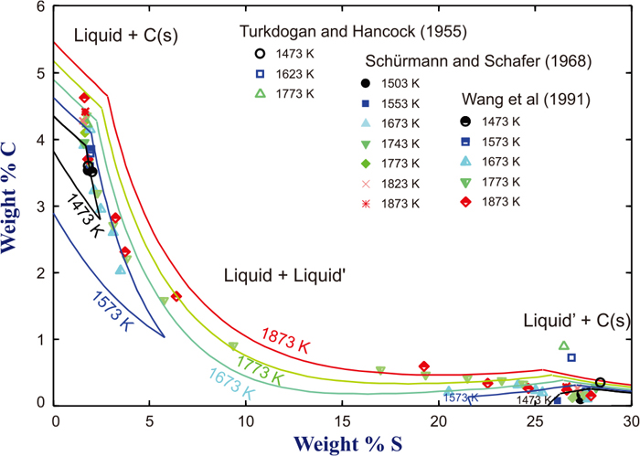
4.1. Miscibility Gap

Experimentally determined miscibility gap in the Fe–C–S liquid at 1823 K is shown in Fig. 1.^13,14,15) Tie-lines connecting compositions of two liquids in equilibrium are also indicated by dotted lines. Those investigations employed high temperature equilibration followed by chemical analysis of immiscible samples, L (C-rich) and L’ (S-rich) liquids, respectively. Turkdogan and Hancock¹³⁾ measured equilibrium composition of the two-liquid in equilibrium with graphite. On the other hand, Schürmann and Schafer,¹⁴⁾ and Wang et al.¹⁵⁾ measured liquid composition of two immiscible liquids when C was not saturated. The latter forms miscibility gap of the ternary liquid at 1773 K. Composition of the miscibility gap at various temperatures are shown in Fig. 2, including those shown in the Fig. 1 by the same authors.^13,14,15) For the sake of simplicity, tie-lines are not shown. The loci of miscibility gap at different temperatures are not very different.

Fig. 1.

Isothermal section of Fe–C–S system at 1773 K showing miscibility gap between L (C-rich metallic liquid) and L’ (S-rich ionic liquid). Symbols and dotted lines are experimentally determined compositions and tie-line, respectively.^13,14,15) Full lines and dashed lines are calculated isothermal section and tie-line, respectively, in the present study. (Online version in color.)

Fig. 2.

Miscibility gap of Fe–C–S system at various temperatures. Symbols are experimentally determined compositions.^13,14,15) Lines are calculated isothermal sections in the present study. (Online version in color.)

In order to reproduce these miscibility gap data, model parameter of the liquid phase was optimized. As discussed in Sec. 3.1, Eq. (17) was added to the Gibbs energy of liquid phase estimated from Gibbs energy of sub-binary liquid phases (Eq. (7)). The added parameters contain three terms:   

$$L_{\text{FeCS}}=-167\hspace{0.17em}360X_{\text{S}}+167\hspace{0.17em}360X_{\text{Fe}}+209 200X_{\text{C}}\text{(J/mol)}$$(19)

in order to reproduce the wide miscibility gap. The present calculations are shown by full lines (miscibility gap and phase boundary) and dashed lines (tie-line). As seen in the Figs. 1 and 2, the overall size of miscibility gap and the direction of tie-line calculated in the present study are favorable agreement with the experimental data.^13,14,15) The present calculation results in slightly higher S content in the L, compared to the reported data.^14,15) The agreement with the experimental data could be improved by adjusting the L_FeCS parameter more positive. However, this adjustment simultaneously deteriorated the other calculation for activity coefficient in the liquid^16,17,18) as will be discussed in Sec. 4.2. Because both set of experimental data are solely determined by the Gibbs energy of liquid phase, there may be inconsistency between the miscibility gap (phase diagram) data and the activity coefficient (thermodynamic) data. In the present study, the activity data^16,17,18) were given more weight, and the reason is discussed in the Sec. 4.2.

Figure 3 shows experimentally determined solubility limit of graphite in C-rich liquid Fe–C–S (L),^{13,14,15,30,31,32)} thereby showing liquidi of graphite at various temperature. Since the Gibbs energy of graphite phase has been well established,²⁶⁾ calculation of the liquidi solely depends on the Gibbs energy of the liquid phase. The present calculation are in good agreement with the experimental data reported by several authors in the temperature range of 1473 K to 1873 K.^{13,14,15,30,31,32)} It is well known that increasing S content decreases the solubility of C in the liquid. This is because of the strong repulsion between C and S, also represented by the wide miscibility gap as seen in the Figs. 1 and 2. Dashed lines at high S content represent not the liquidi of graphite, but the miscibility gap at each temperature. Most of the experimental data fall in the region of L + graphite.

Fig. 3.

Isothermal sections of Fe–C–S system at low S region, showing solubility limit of graphite in liquid at various temperatures. Symbols are experimentally determined compositions.^{13,14,15,30,31,32)} Lines are calculated isothermal sections in the present study. Right hand side of the figure represents miscibility gap in the liquid phase. (Online version in color.)

4.2. Activity of S in Liquid Phase

Figure 4 shows activity coefficient of S in Fe–C–S liquid at each temperature (1473 K to 2073 K).^16,17,18) The activity coefficient (fs) refers to 1 wt% standard state of S in liquid Fe, and it was calculated using the following reaction and Gibbs energy change evaluated in the present study:   

$$\frac{1}{2}{\text{S}}_2\left(\text{g}\right)=\underset{\_}{\mathrm{S}};\mathrm{\hspace{0.17em} }\mathrm{\hspace{0.17em} }\mathrm{\hspace{0.17em} }\mathrm{\Delta }{g}_{\underset{\_}{\mathrm{S}}}^{°}=-105\mathrm{\hspace{0.17em} }461+8.165T\left(\text{J}\cdot {\text{mol}}^{-1}\right)$$(20)

where a procedure of the evaluation of the Gibbs energy is discussed in Appendix A.

Fig. 4.

Activity coefficient of S in Fe–C–S liquid alloys at various temperatures, with respect to 1 wt% standard state. Symbols are experimentally determined data.^16,17,18) Full lines are calculated activity coefficient in the present study at 0.001 wt% S (close to infinite dilution). Dotted line in (e) is from Sigworth and Elliott.³⁴⁾

Experimental data of Morris and Buehl,¹⁶⁾ Ban-ya and Chipman,¹⁷⁾ and Ishii and Fuwa¹⁸⁾ were measured for homogeneous liquid Fe–C–S in equilibrium with H₂S–H₂ gas mixture in order to fix partial pressure of S₂(g). By the reaction (20), the activity of S in the liquid, as one of the thermodynamic properties of the liquid phase, could be obtained. Therefore, dependence of fs on carbon content thus represents solution thermodynamics of the liquid phase. From the figure, it is seen that increasing C content increases the fs, as expected from the shape of phase diagrams (Figs. 1, 2, 3). The solid lines are calculated in present study. In order to fit the experimental data of fs, the ternary model parameter L_FeCS (Eq. (19)) was optimized. As mentioned in Sec. 4.1, the fs shown in Fig. 4 and the miscibility gap data shown in Figs. 1 and 2 were found to be inconsistent each other. Using the thermodynamic model, it was not possible to reproduce both set of experimental data. To the present authors’ opinion, experimental investigation of the miscibility gap was more difficult because 1) rapid quenching to separate two liquids, L (C-rich) and L’ (S-rich), might be difficult, and 2) rapid evaporation of carbosulfide gas species (CS(g), CS₂(g))^5,33) at high C content could cause less S content than actual equilibrium content. Therefore, in the present study, more weight was given to the experimental investigation of fs, and the ternary model parameter L_FeCS was optimized in order to reproduce both set of experimental data, in particular for the fs. The present calculation is in good agreement with the most experimental data, except at 2073 K. As mentioned before, possible evaporation loss of S due to carbosulfide gas species (CS(g), CS₂(g)) might cause lower S content in the liquid, yielding higher fs. Therefore, the data at 2073 K was not used in the present optimization.

A dotted line shown in Fig. 4(e) was calculated using Wagner’s Interaction Parameter Formalism (WIPF) along with the recommended first order ($e_{\text{S}}^{\text{C}}$) and second order interaction parameter ($r_{\text{S}}^{\text{C}}$):^8,34)   

$$\text{log}{f}_{\text{S}}=e_{\text{S}}^{\text{C}}[\text{\%C}]+r_{\text{S}}^{\text{C}}{[\text{\%C}]}^2$$(21)

where $e_{\text{S}}^{\text{C}}$=0.11 and $r_{\text{S}}^{\text{C}}$=0.0058, respectively.

Both calculations agree well each other and agree with the experimental data of Morris and Buehl at 1873 K.¹⁶⁾ The recommended interaction parameters by Sigworth and Elliott³⁴⁾ looks very reasonable, although its use was limited at 1873 K. In the present study, the fs calculated using the present thermodynamic model from 1473 K to 2073 K, from 0 wt% C to carbon saturation (~6 wt%) (shown in the Fig. 4 by full lines) was analyzed by fitting the calculated results to the WIPF, in order to provide the $e_{\text{S}}^{\text{C}}$ and $r_{\text{S}}^{\text{C}}$ to be used at the wider condition:   

$$\begin{array}{l}{e}_{\text{S}}^{\text{C}}=\frac{23}{T}+0.0803,\mathrm{\hspace{0.17em} }\mathrm{\hspace{0.17em} }\mathrm{\hspace{0.17em} }{r}_{\text{S}}^{\text{C}}=\frac{26}{T}-0.0045\\ \left(1\mathrm{\hspace{0.17em} }473\mathrm{\hspace{0.17em} }\mathrm{K}<\mathrm{T}<2\mathrm{\hspace{0.17em} }073\mathrm{\hspace{0.17em} }\mathrm{K}\right)\end{array}$$(22)

4.3. Phase Diagrams

Figure 5 shows liquidus of γ in the temperature range of 1523 K to 1673 K. Experimental data from Schürmann and Schafer¹⁴⁾ and Vogel and Ritzau³⁵⁾ are shown by symbols. Since the γ is mostly composed of Fe and C and content of S in the γ phase is low (maximum 0.05 wt%),²⁹⁾ effect of S on the Gibbs energy of the ternary γ is negligible. Therefore, it was not attempted to adjust any model parameters relevant ternary Fe–C–S interaction in the γ phase, as well as those of bcc phase (α and δ phases). Shown in the Fig. 5 is the calculated liquidus of the γ phase. It is seen that there is a good agreement between the model calculation and the experimental data. This also supports the present thermodynamic modeling of the liquid phase.

Fig. 5.

Liquidi of γ in Fe–C–S system at various temperatures. Symbols are experimentally determined compositions.^14,35) Lines are calculated isothermal sections in the present study. (Online version in color.)

Figure 6 show three isoplethal sections of the Fe–C–S system at 0.02, 2 and 5 wt% S, respectively. Experimental data of Ohtani and Nishzawa,¹¹⁾ Vogel and Ritzau³⁵⁾ were compared with the present model calculation. In Figs. 6(b) and 6(c), it is seen that liquidus of γ phase (even in the presence of S-rich liquid L’) is well reproduced by the present model calculations. However, a eutectic reaction (L → L’ + γ + C(s)) calculated in the present study takes place at higher temperature (1401 K) than the reported temperature (1373 K). Consideration of metastable phase equilibria involving Fe₃C (shown by dashed lines) did not correct the discrepancy. A previous thermodynamic analysis by Ohtani and Nishizawa¹¹⁾ also showed a bit higher eutectic temperature, which looks close to the present result. Since the eutectic reaction involves either almost binary phases (L, γ, and Fe₃C of low S content, L’ of low C content) or pure material (graphite), it is not easy to adjust the Gibbs energy of those phases using ternary parameters. This requires further investigation.

Fig. 6.

Isoplethal sections of Fe–C–S system at (a) 0.02, (b) 2, and (c) 5 wt% S, respectively. Symbols in b) and c) are experimentally determined thermal arrests.^11,35) Full lines and dashed lines are calculated isoplethal sections of stable phase diagram (graphite as the stable phase) and metastable phase diagram (cementite as the stable phase), respectively, in the present study. (Online version in color.)

Ohtani and Nishizawa¹¹⁾ carried out an experiment to observe a remelting phenomena of this alloy system. They heat treated a number of alloys of 0.93%C–0.02%S at various temperatures, quenched followed by microscopic observation. Their observation is shown in Fig. 6(a). Some of their alloys at low temperature were found to be partially melted (1273, 1323, 1373 K), while the other alloy at higher temperatures (1423 and 1573 K) were not melted. Such melting at the low temperature was different from the melting at the highest temperature at 1623 K. According to their thermodynamic analysis, this remelting was due to appearance of S-rich liquid (L’), which is different to the C-rich metallic liquid (L). In the present study, a similar result was obtained by the thermodynamic calculation. The present thermodynamic calculation results in the remelting at 1351 K, while Ohtani and Nishizawa observed the remelting even at 1373 K. It is thought that the sample heat treated at 1373 K might have melted during quenching by passing through the L’ + γ region.

Finally, Fig. 7 shows a calculated liquidus projection of the Fe–C–S system at Fe-rich corner. Two invariant reactions and one maximum on a monovariant line is predicted, as listed in Table 3. An additional invariant reaction (eutectoid reaction) is also predicted as listed in the Table 3. The calculated liquidus projection at high temperature region (approximately higher than 2273 K) is not certain, and it is shown by dashed lines.

Fig. 7.

Calculated liquidus surface of the Fe–C–S system in the present study, showing two invariant reactions and one maximum on a monovariant line. See Table 3. (Online version in color.)

Table 3. Special reactions in the Fe–C–S system.

Reaction	Typea	T (K)	Compositionb		Reference
			%C	%S
L → L’ + γ + C(s)	m	1401	3.76	1.48	Present study
	m	1373	3.2	1.9	Ref. 14)
L + L’ → γ + C(s)	q	1401	0.22	28.48	Present study
	m	1373	0.1	27.6	Ref. 14)c
L → L’ + γ	M	1619	0.09	13.44	Present study
	M	1573	0.3	14.8	Ref. 14)
L → γ + C(s) + Fe1−xS	e	1266	0.15	31.08	Present study
	e	1248	0.1	31.0	Ref. 14)
γ → α + Fe1−xS + C(s)	ed	1011	0.068	0.00098	Present study
	ed	998	-	-	Ref. 10)
a: m (monotectic), q (quasi-peritectic), M (maximum), ed (eutectoid), e (eutectic)
b: L or γ
c: reported as L’ → L + γ + C(s)

5. Conclusions

In order to provide accurate description for the activity of components in liquid Fe–C–S solution over wide concentration and temperature range, a critical evaluation and thermodynamic optimization of the Fe–C–S system were carried out using CALPHAD type thermodynamic modeling approach. In order to take into account very strong attraction between Fe and C, and between Fe and S in the liquid phase, previously used thermodynamic model (MQM) was used in the present study. However, in order to explain very strong repulsion between C and S in the liquid, a Bragg-William type ternary parameter, X_FeX_CX_SL_FeCS, was introduced in the Gibbs energy model equation for the liquid phase. Use of this type of interaction energy in the MQM was previously proposed by Kang and Pelton.²⁸⁾ Using the ternary parameter in the liquid phase, wide miscibility gap in the liquid phase and the activity coefficient of S increased by C were modeled reasonably. As a result, the following interaction parameter was obtained:   

$$e_{\text{S}}^{\text{C}}=\frac{23}{T}+0.0803,\mathrm{\hspace{0.17em} }\mathrm{\hspace{0.17em} }\mathrm{\hspace{0.17em} }{r}_{\text{S}}^{\text{C}}=\frac{26}{T}-0.0045$$(22)

which can be used in the temperature range of 1473 K to 2073 K. During the evaluation of the interaction parameter, a Gibbs energy change for a reaction:   

$$\frac{1}{2}{\text{S}}_2\left(\text{g}\right)=\underset{\_}{\mathrm{S}};\mathrm{\hspace{0.17em} }\mathrm{\hspace{0.17em} }\mathrm{\hspace{0.17em} }\mathrm{\Delta }{g}_{\underset{\_}{\mathrm{S}}}^{°}=-105\mathrm{\hspace{0.17em} }461+8.165T\left(\text{J}\cdot {\text{mol}}^{-1}\right)$$(20)

is proposed by analyzing the previous thermodynamic modeling of the Fe–S binary liquid by Waldner and Pelton.²²⁾

The presently developed thermodynamic database can also be used to calculate various phase diagrams in this ternary system. Also, it can be further extended into multicomponent system including Fe, C, and S.

Appendix A.

Evaluation of Gibbs Energy Change for the Reaction 1/2S₂(g)=S Using the Thermodynamic Assessment of Waldner and Pelton²²⁾

During the calculation of the activity coefficient of S in liquid Fe–C–S alloys in 1 wt% standard state (f_S) as shown in Fig. 4, the Gibbs energy change for the Reaction (20) was not taken from the recommendation of JSPS which has been generally used.⁸⁾ Instead, the Gibbs energy change was separately evaluated in the present study using the thermodynamic assessment of Waldner and Pelton.²²⁾ All the experimental data and thermodynamic calculations shown in the Fig. 4 were then manipulated using the $\mathrm{\Delta }{g}_{\underset{\_}{\mathrm{S}}}^{°}$ in order to obtain the f_S. This was done in order to compare the f_S from the experiments^16,17,18) and that from the present thermodynamic calculation, at the same standard state.

The Gibbs energy change for the Reaction (20) represents Gibbs energy difference between the 1 wt% standard state, g_S,1wt% and pure S₂ (g), $g_{{\mathrm{S}}_2}^{°}$:   

$$\mathrm{\Delta }{g}_{\underset{\_}{\mathrm{S}}}^{°}=g_{\underset{\_}{\mathrm{S}},1\text{wt\%}}-\frac{1}{2}{g}_{{\text{S}}_2}^{°}$$(A.1)

where the $g_{{\mathrm{S}}_2}^{°}$ is a property of pure S₂ gas, but the g_S,1wt% is a solvent dependent value. In the present case, it represents the Gibbs energy of a solution composed of Fe and S at 1 wt% S, along with Henrian activity coefficient of S (${\gamma }_{\mathrm{S}}^{°}$) in a infinitely diluted liquid Fe–S alloy. Therefore, its Gibbs energy is expressed as:   

$$\begin{array}{c}{g}_{\underset{\_}{\mathrm{S}},1\text{wt\%}}=g_{\text{S}}^{°,l}+\text{R}T\hspace{0.17em}\text{ln}\left({\gamma }_{\text{S}}^{°}\frac{\raisebox{1ex}{$1$}\!\left/ \!\raisebox{-1ex}{$M_{\text{S}}$}\right.}{\raisebox{1ex}{$99$}\!\left/ \!\raisebox{-1ex}{$M_{\text{Fe}}$}\right.+\raisebox{1ex}{$1$}\!\left/ \!\raisebox{-1ex}{$M_{\text{S}}$}\right.}\right)\\ \approx g_{\text{S}}^{°,l}+\text{R}T\hspace{0.17em}\text{ln}\left({\gamma }_{\text{S}}^{°}\frac{M_{\text{Fe}}}{100M_{\text{S}}}\right)\end{array}$$(A.2)

where M_i is a molecular weight of a component i. Therefore, $\mathrm{\Delta }{g}_{\underset{\_}{\mathrm{S}}}^{°}$ is dependent on the ${\gamma }_{\mathrm{S}}^{°}$, which is the solvent dependent property. Since the present thermodynamic modeling for the Fe–C–S liquid employed the previous thermodynamic modeling for the Fe–S by Waldner and Pelton,²²⁾ using the ${\gamma }_{\mathrm{S}}^{°}$ from the work of Waldner and Pelton should give a consistent definition of the $\mathrm{\Delta }{g}_{\underset{\_}{\mathrm{S}}}^{°}$ of the Reaction (20). Calculated ${\gamma }_{\mathrm{S}}^{°}$ from the work of Waldner and Pelton²²⁾ at various temperatures are shown in Fig. A.1, and it was fitted to a function of temperature:   

$$\text{ln}{\gamma }_{\mathrm{S}}^{°}=-\frac{7 \hspace{0.17em}630}{T}-1.1465$$(A.3)

Fig. A.1.

Henrian activity coefficient of S (${\gamma }_{\mathrm{S}}^{°}$) in liquid Fe–S alloy at various temperatures. Symbols are calculated values from the thermodynamic assessment of Waldner and Pelton.²²⁾ (Online version in color.)

The Eq. (A.3) was substituted into the Eq. (A.2) in order to obtain g_S,1wt%, and subsequently into the Eq. (A.1). This results in the $\mathrm{\Delta }{g}_{\underset{\_}{\mathrm{S}}}^{°}$:   

$$\frac{1}{2}{\text{S}}_2\left(\text{g}\right)=\underset{\_}{\mathrm{S}};\mathrm{\hspace{0.17em} }\mathrm{\hspace{0.17em} }\mathrm{\hspace{0.17em} }\mathrm{\Delta }{g}_{\underset{\_}{\mathrm{S}}}^{°}=-105\mathrm{\hspace{0.17em} }461+8.165T\left(\text{J}\cdot {\text{mol}}^{-1}\right)$$(20)

On the other hand, JSPS recommended to use the following:⁸⁾   

$$\frac{1}{2}{\text{S}}_2\left(\text{g}\right)=\underset{\_}{\text{S}};\mathrm{\hspace{0.17em} }\mathrm{\hspace{0.17em} }\mathrm{\hspace{0.17em} }\mathrm{\Delta }{g}_{\underset{\_}{\mathrm{S}},\text{JSPS}}^{°}=-125 \mathrm{\hspace{0.17em} }100+18.5T\left(\text{J}\cdot {\text{mol}}^{-1}\right)$$(A.4)

which was assessed using experimental data of Ishii and Fuwa who measured the equilibrium S content in the liquid Fe–C–S alloy under controlled H₂S–H₂ gas mixture by resistance furnace in the temperature range of 1773 K to 1873 K.³⁶⁾ These two Gibbs energies are compared in Fig. A.2. As seen in the figure, these two sets of Gibbs energies are close about 1873 K, but show noticeable discrepancy at low temperature, where high C hot metal could be molten state. Since Waldner and Pelton did utilize the experimental data for Ishii and Fuwa³⁶⁾ during their thermodynamic assessment,²²⁾ it is seen that these two sets of Gibbs energies look to favorably agree each other in the temperature range of the experimental investigation of Ishii and Fuwa.³⁶⁾ In addition to this, Waldner and Pelton also took into account 1) activity of S in Fe–S liquid solution at lower temperature down to 1373 K when S concentration was high, 2) phase diagram data (equilibrium with δ and with γ). These considerations should have resulted in Gibbs energy of the liquid Fe–S phase being accurately evaluated even at low temperature (~1273 K where the liquid solidifies). Therefore, the full line in Fig. A.2 (Eq. (20)) is considered to be assessed even at low temperature, not extrapolated as the dashed line (Eq. (A.4)) is.

Fig. A.2.

Gibbs energy change for the reaction 1/2S₂ (g) = S(1 wt%) as a function of temperature: dashed line from JSPS⁸⁾ and full line evaluated in the present study using the ${\gamma }_{\mathrm{S}}^{°}$ shown in Fig. A.1. (Online version in color.)

Figure A.3 shows the f_S, both experimental data and the calculation in the present study (at 0.001 wt% S (close to infinite dilution)), using the $\mathrm{\Delta }{g}_{\underset{\_}{\mathrm{S}},\text{JSPS}}^{°}$ for the conversion of the standard state to 1 wt% standard state (Eq. (A.4)). When this is compared with the Fig. 4, f_S does not converge to unity when wt% C is zero (thus, infinite dilution of S), in particular at low temperature (1473 K to 1688 K). This is due to the use of inconsistent set of thermodynamic data (${\gamma }_{\mathrm{S}}^{°}$ from Waldner and Pelton as used in the present thermodynamic modeling, while $\mathrm{\Delta }{g}_{\underset{\_}{\mathrm{S}},\text{JSPS}}^{°}$ from JSPS which uses a different ${\gamma }_{\mathrm{S}}^{°}$). Using the inconsistent set of thermodynamic data resulted in considerable error in the calculation of f_S. The error caused by such inconsistent combination is seen in Fig. A.3(a) as an example.

Fig. A.3.

Activity coefficient of S in Fe–C–S liquid alloys at various temperatures, with respect to 1 wt% standard state using $\mathrm{\Delta }{g}_{\underset{\_}{\mathrm{S}},\text{JSPS}}^{°}$ from JSPS.⁸⁾ Legends are the same to those in Fig. 4. (Online version in color.)

Therefore, it is concluded that the $\mathrm{\Delta }{g}_{\underset{\_}{\mathrm{S}},\text{JSPS}}^{°}$ may not be used with the present thermodynamic modeling result in order to calculate f_S in liquid Fe–C–S at low temperature which is relevant to pig iron production and hot metal pretreatment. Moreover, the Eq. (20), which was evaluated in the present study using the thermodynamic assessment of Waldner and Pelton, is seen to be in favorable agreement not only with the Eq. (A.4) of the $\mathrm{\Delta }{g}_{\underset{\_}{\mathrm{S}},\text{JSPS}}^{°}$ about 1823 K to 1873 K, but also is in good agreement with the experimental data at low temperature as shown in Fig. 4. It is also thermodynamically consistent with the present thermodynamic modeling result presented in this article.

References

• 1)   C.  Wang,  T.  Nagasaka,  M.  Hino and  S.  Ban-Ya: ISIJ Int., 31 (1991), 1300.
• 2)   C.  Wang,  T.  Nagasaka,  M.  Hino and  S.  Ban-Ya: ISIJ Int., 31 (1991), 1309.
• 3)   S.-H.  Jung,  Y.-B.  Kang,  J.-D.  Seo,  J.-K.  Park and  J.  Choi: Metall. Mater. Trans. B, 46B (2015), 250.
• 4)   S.-H.  Jung,  Y.-B.  Kang,  J.-D.  Seo,  J.-K.  Park and  J.  Choi: Metall. Mater. Trans. B, 46B (2015), 259.
• 5)   S.-H.  Jung,  Y.-B.  Kang,  J.-D.  Seo,  J.-K.  Park and  J.  Choi: Metall. Mater. Trans. B, 46B (2015), 267.
• 6)   S.-H.  Jung and  Y.-B.  Kang: Metall. Mater. Trans. B, 47B (2016), 2164.
• 7)   S.-H.  Jung and  Y.-B.  Kang: Metall. Mater. Trans. B, 47B (2016), 2564.
• 8)  Japan Society for the Promotion of Science: Steelmaking Data Source Book, Gordon and Breach Science Publishers, Montreux, (1984).
• 9)   F.  Tafwidli: M.Sc. thesis, POSTECH, (2017).
• 10)   V.  Raghavan: Phase Diagrams of Ternary Iron Alloys. Part 2: Ternary Systems Containing Iron and Sulphur, Indian Institute of Metals, Calcutta, (1988), 73.
• 11)   H.  Ohtani and  T.  Nishizawa: Trans. Iron Steel Inst. Jpn., 26 (1986), 655.
• 12)   V.  Raghavan: J. Phase Equil., 19 (1998), 262.
• 13)   E. T.  Turkdogan and  R. A.  Hancock: J. Iron Steel Inst., 179 (1955), 155.
• 14)   E.  Schürmann and  K.  Schafer: Giessenreiforschung, 20 (1968), 21.
• 15)   C.  Wang,  J.  Hirama,  T.  Nagasaka and  S.  Ban-Ya: ISIJ Int., 31 (1991), 1292.
• 16)   J. P.  Morris and  R. C.  Buehl: Trans. AIME, 188 (1950), 317.
• 17)   S.  Ban-Ya and  J.  Chipman: Trans. AIME, 245 (1969), 133.
• 18)   F.  Ishii and  T.  Fuwa: Tetsu-to-Hagané, 67 (1981), 746.
• 19)   M.  Hillert: J. Alloys. Compd., 320 (2001), 161.
• 20)   M.  Hillert and  M.  Jarl: Calphad, 2 (1978), 227.
• 21)   A. D.  Pelton,  S.  Degterov,  G.  Eriksson,  C.  Robelin and  Y.  Dessureault: Metall. Mater. Trans. B, 31B (2000), 651.
• 22)   P.  Waldner and  A. D.  Pelton: J. Phase Equil. Diffus., 26 (2005), 23.
• 23)   K.  Shubhank and  Y.-B.  Kang: Calphad, 45 (2014), 127.
• 24)   C. W.  Bale,  E.  Belisle,  P.  Chartrand,  S. A.  Decterov,  G.  Eriksson,  K.  Hack,  I.-H.  Jung,  Y.-B.  Kang,  J.  Melancon,  A. D.  Pelton,  C.  Robelin and  S.  Petersen: Calphad, 33 (2009), 295.
• 25)   C. W.  Bale,  E.  Belisle,  P.  Chartrand,  S. A.  Decterov,  G.  Eriksson,  A. E.  Gheribi,  K.  Hack,  I.-H.  Jung,  Y.-B.  Kang,  J.  Melancon,  A. D.  Pelton,  S.  Petersen,  C.  Robelin,  J.  Sangster,  P.  Spencer and  M.-A.  Van Ende: Calphad, 54 (2016), 35.
• 26)   A. T.  Dinsdale: Calphad, 15 (1991), 317.
• 27)   A. D.  Pelton and  P.  Chartrand: Metall. Mater. Trans. A, 32A (2001), 1355.
• 28)   A. D.  Pelton and  Y.-B.  Kang: Int. J. Mater. Res., 98 (2007), 907.
• 29)   P.  Gustafson: Scand. J. Metall., 14 (1985), 259.
• 30)   P. O.  Mellberg and  L.  Yunzu: Scand. J. Metall., 10 (1981), 94.
• 31)   M.  Ohtani and  N. A.  Gokcen: Trans. AIME, 218 (1960), 380.
• 32)   T.  Mori,  T.  Ogasawara,  H.  Hasegawa,  T.  Hatakeyama and  T.  Yamada: Tetsu-to-Hagané, 46 (1960), 101.
• 33)   R.  Ohno: J. Jpn. Inst. Met., 23 (1959), 489.
• 34)   G. K.  Sigworth and  J. F.  Elliott: Met. Sci., 8 (1974), 298.
• 35)   R.  Vogel and  G.  Ritzau: Arch. Eisenhuettenwes., 4 (1931), 549.
• 36)   F.  Ishii and  T.  Fuwa: Tetsu-to-Hagané, 67 (1981), 736.