Nanostructural Analyses of Intra- and Intergranular Precipitates in High-temperature Heat-treated Nitrogen-added Austenitic Stainless Steel

Abstract

More than one thousand intragranular and intergranular precipitates of nitrogen-added austenitic stainless steel, SUSXM15J1, were characterized by FIB-SEM serial-sectioning tomography, by conventional transmission electron microscopy (TEM) and by scanning transmission electron microscopy (STEM). All of intragranular precipitates were found nitrided to form dichromium nitride, Cr₂N, two types of intergranular precipitates were found Cr₂N and Cr₃Ni₂Si(N), and some of them were grown and jointed due to the additional heat treatment during the tensile test at 1173 K, which probably contributed to its high-temperature strength.

1. Introduction

Austenitic stainless steels are widely used in engineering applications due to their superior corrosion resistance,^1,2) weldability,³⁾ and mechanical properties.^4,5,6) It is known that the corrosion resistance and the mechanical properties are influenced by alloying elements, and in particular nitrogen is commonly added to austenitic stainless steels because it improves mechanical properties and corrosion resistance, and stabilization of austenite.⁷⁾ Addition of nitrogen is very effective method for improving normal and high temperature strength, probably due to its solid-solution strengthening by interstitial-substitutional effect,^8,9) the interaction between solute atoms and the faulted area of extended dislocations being dominant known as Suzuki effect.¹⁰⁾ In addition, consequential precipitate formation, in which precipitates would act as the pinning cites for dislocations and results the precipitation hardening.¹¹⁾ These proposed mechanisms have not been confirmed yet, so that it is still necessary to investigate the nitrogen-added samples at nanoscale to determine the role of nitrogen, and to improve the physical properties of austenitic stainless steel. The precipitation hardening mechanisms have been generally understood that the deformation mechanism changes from cutting to Orowan looping of dislocations, due to the sizes, morphologies, dispersions and structures of precipitates.^12,13,14,15) Furthermore, the interactions between precipitates and dislocations under high temperature, as well as modifications of nanostructures, are still poorly understood, so that the quantitative and qualitative analyses of them are inevitable.

In this paper, both FIB-SEM serial-sectioning method and (S)TEM characterization were applied on the nitrogen-added austenitic stainless steel (SUSXM15J1), to characterize the intra- and intergranular precipitates, in detail.

2. Experimental

2.1. Samples

The composition of the steel used in this study is listed in Table 1.

Table 1. Chemical composition of SUSXM15J1 investigated (wt.%).

C	Si	Mn	P	Ni	Cr	S	N
0.05	3.2	0.8	0.03	13.5	19.5	0.0007	0.19

20 kg of Si-added austenitic stainless steel, SUSXM15J1, with 0.19% of nitrogen was prepared by vacuum melting, forged to 55 mm at 1523 K, and ground to 40 mm at R.T. Furthermore, the sample was heated at 1423 K for 1 hour, rolled to 6 mm, annealed at 1423 K for 60 seconds, and air cooled. The cooled sample was rolled to prepare 2 mm thick sample, then annealed at 1423 K for 60 seconds, and air cooled. A test piece for high temperature tensile test with its dimension 10 mm width and 35 mm gauge length was cut from the sheet, where tensile direction was set parallel to the rolling direction. The high temperature tensile test was carried out at 1173 K for 20 minutes, with tensile speed at 0.3%/min, and 3 mm/min after 0.2% proof stress until the fracture, then cooled. In this study, gripping part with less dislocation and strain was then mechanically polished for SEM observation and FIB-SEM serial-sectioning tomography because the main purpose is to observe precipitates.

2.2. Three-dimensional Analyses by FIB-SEM Serial-Sectioning Tomography

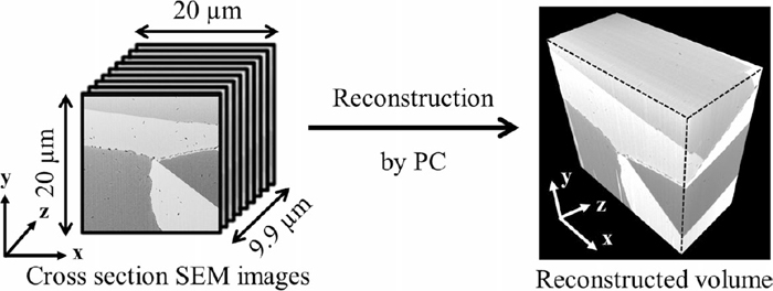
FIB-SEM serial-sectioning tomography was performed by a dual beam FIB, SMF-1000 (Hitachi High-Tech Science Corp., Japan), in which FIB and SEM columns are arranged perpendicularly to achieve high contrast and high resolution.¹⁶⁾ The sample was ion-milled by Ga⁺ beam at an acceleration voltage of 30 kV with ion current of 3.0 nA, then each cross-sectional image was obtained by SEM. The acceleration voltage was at 1.0 kV for the acquisition of SEM images, using mixture of two detectors, for secondary and backscattered electrons.

Layers of 10 nm were milled in each step during the serial-sectioning procedure and repeated until 990 successive images were collected. The off-line alignment of images, the volume segmentation, the visualization and the quantification were then performed by commercial software, Amira 6.2 (Thermo Fisher Scientific, USA), respectively. The drift in the x- and y-directions were corrected during the off-line data processing by applying least square fitting algorithms to achieve alignment of the images in the stack, as shown in Fig. 1.

Fig. 1.

A schematic diagram of FIB-SEM slice-sectioning method.

2.3. TEM and STEM Observation

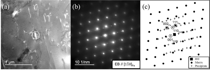
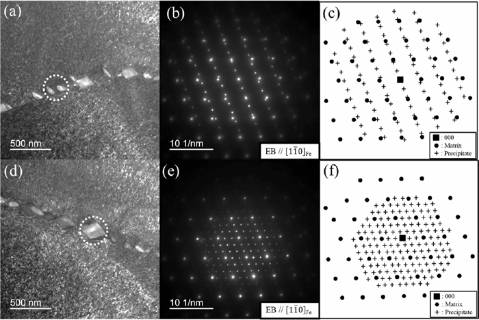
Both structural and analytical TEM experiments were carried out by JEM-ARM-200F (JEOL, Japan) operated at 200 kV. TEM sample was prepared from the same field of view of the FIB-SEM serial-sectioning, which was picked up and thinned by FIB. Selected area electron diffraction (SAED) patterns were obtained from intra- and intergranular precipitates at 80 cm of camera length, and electron beam direction set to [110] of matrix (γ-Fe).

Two-dimensional elemental distribution maps were acquired via the combination of scanning transmission electron microscopy and energy dispersive X-ray spectroscopy (STEM-EDS) using X-ray analyzer (JED-2300T of JEOL), a drift-correcting and visualizing program (Analysis Station of JEOL).

3. Results and Discussion

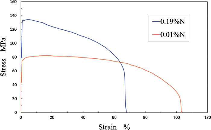
Figure 2 shows the stress-strain curve of 0.19%N sample and 0.01%N sample, tensile tested under the same conditions. As clearly seen from these curves, it was confirmed that the tensile strength was increased by addition of nitrogen at high temperature. In particular, 0.2% yield strength and tensile strength of 0.19% N samples are 84 MPa and 133 MPa, respectively, and those of 0.01% N material are 44 MPa and 81 MPa, respectively. From these results, it was confirmed that 0.2% proof stress at 1173 K was improved by 40 MPa and tensile strength by 52 MPa via addition of 0.19% N, and high temperature strength at 1173 K was also improved. Moreover, it showed the similar tendency as previously reported results that the 0.2% proof stress at 1173 K of austenitic stainless steels increased almost linearly with the increase of nitrogen content, as about 3 MPa per addition of 0.01%.¹⁷⁾ Although the elongation at fracture of 0.19% N sample is more than 60% but less than that of 0.01% N material, and it is probably caused the inhomogeneity of microstructures due to formation of planar dislocation arrays.¹⁸⁾

Fig. 2.

S-S curves about 0.01%N and 0.19%N sample. (Online version in color.)

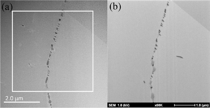
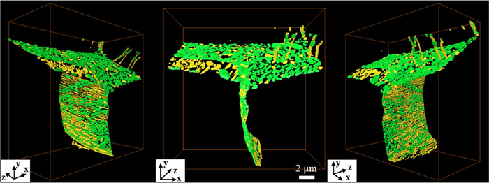
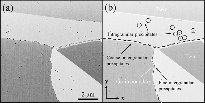
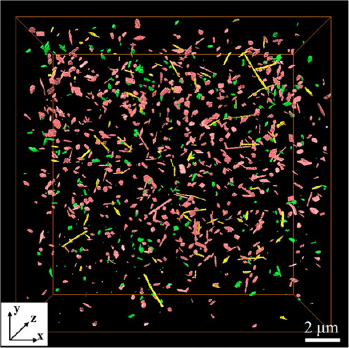
One of the successive cross-sectional SEM images of FIB-SEM serial-sectioning tomography and its schematic diagram are shown in Figs. 3(a) and 3(b), respectively. It was confirmed that there were a large number of both intra- and intergranular precipitates in the field of view, with grain boundaries, triple points, and twin boundaries. A representative three-dimensionally reconstructed volume with more than 1000 intragranular precipitates is shown in the field, 20 μm × 20 μm × 9.9 μm, seeing from different orientations as shown in Fig. 4.

Fig. 3.

(a) shows a part of the continuous cross section SEM image and (b) its schematic diagram of contrasts.

Fig. 4.

A set of images of intragranular precipitates seeing from different orientations. (Online version in color.)

3.1. Intragranular Precipitates

Almost homogeneously dispersed intragranular precipitates are color-coded to differentiate plate-type (red), rod-type (yellow) and granular-type (green) precipitates, as shown in Fig. 5, with their average size, average volume and number (ratio), as summarized in Table 2. From these results, it was clarified that the number of plate-type precipitates are largest, and the volume of rod-type precipitates are found largest.

Fig. 5.

The three-dimensional reconstructed image color-coded by the shape of the intragranular precipitates. (Online version in color.)

Table 2. Quantified results of intragranular precipitates.

In addition, it was clearly seen that there would have been clear orientation relationships between the precipitates and matrix, since the growth direction of plate-type precipitates being linear when they were seeing from particular directions, as shown in Fig. 6.

Fig. 6.

The image of plate-type intragranular precipitates has specific growth direction. (Online version in color.)

3.1.1. Plate-type

A set of bright-field (BF)-TEM image and SAED pattern of a representative plate-type intragranular precipitates are shown in Figs. 7(a) and 7(b), respectively. The average size of plate-type intragranular precipitates are measured as 460 (longer axis) × 70 (shorter axis) nm. A distinctive crystallographic orientation relationship, partially applicable to the Shoji-Nishiyama relationship, was observed between the plate-type precipitates and the matrix, as schematically shown in Fig. 7(c).

Fig. 7.

(a) BF-TEM image of plate-type intragranular precipitates and (b) SAEDP from the region shown in (a) and (c) schematic diagram of SAEDP.

In general, the Shoji-Nishiyama orientation relationship¹⁹⁾ was observed between h.c.p. and f.c.c.   

$$\begin{array}{l}{\left(111\right)}_{\text{fcc}}\left|\right|{\left(0001\right)}_{\text{hcp}}\text{, }{\left[1\overline{1}0\right]}_{\text{fcc}}\left|\right|{\left[11\overline{2}0\right]}_{\text{hcp}}\\ or\\ {\left(111\right)}_{\text{fcc}}\left|\right|{\left(0001\right)}_{\text{hcp}}\text{, }{\left[11\overline{2}\right]}_{\text{fcc}}\left|\right|{\left[1\overline{1}00\right]}_{\text{hcp}}\end{array}$$

This relationship was partially applicable to the structural relationship between the plate-type precipitates and the matrix as,   

$${\left(111\right)}_{\text{Matrix}}\left|\right|{\left(0001\right)}_{\text{Plate}}\text{, }{\left[1\overline{1}0\right]}_{\text{Matrix}}\left|\right|{\left[1\overline{1}00\right]}_{\text{Plate}}$$

which could be seen from Fig. 7(b).

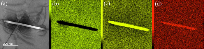
Bright-field (BF)-STEM image and a set of elemental distribution maps of Fe, Cr and N from the plate-type intragranular precipitates are shown in Figs. 8(a), 8(b), 8(c) and 8(d), respectively, where the presences of Cr and N were confirmed. The results of TEM-SAEDP and STEM-EDS confirm that the plate-type precipitates were Cr₂N.

Fig. 8.

A set of (a) BF-STEM image and EDS elemental distribution map of (b) Fe, (c) Cr, and (d) N from the plate-type intragranular precipitate. (Online version in color.)

3.1.2. Rod-type

Bright-field (BF)-TEM image and SAED pattern of a rod-type intragranular precipitates are shown in Figs. 9(a) and 8(b), respectively. The average size of rod-type intragranular precipitates are found 550 (longer axis) × 40 (shorter axis) nm.

Fig. 9.

(a) BF-TEM image of rod-type intragranular precipitates and (b) SAEDP from the region shown in (a) and (c) schematic diagram of SAEDP.

A distinctive crystallographic orientation relationship, again partially applicable to the Shoji-Nishiyama relationship, was also observed between the rod-type precipitates and the matrix, as schematically shown in Fig. 9(c).   

$${\left(111\right)}_{\text{Matrix}}\left|\right|{\left(0001\right)}_{\text{Rod}},{\left[1\overline{1}0\right]}_{\text{Matrix}}\left|\right|{\left[2\overline{1}\overline{1}0\right]}_{\text{Rod}}$$

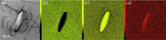
In addition, a set of elemental distribution map, BF-STEM, Fe, Cr and N, is shown in Figs. 10(a), 10(b), 10(c) and 10(d), respectively.

Fig. 10.

A set of (a) BF-STEM image and EDS elemental distribution map of (b) Fe, (c) Cr, and (d) N from the rod-type intragranular precipitate. (Online version in color.)

It is clearly seen that high concentration of Cr and N in precipitates, as in the case of the plate-type precipitate. From these results, the rod-type precipitates are also determined as Cr₂N.

3.1.3. Granular-type

Bright-field (BF)-TEM image and SAED pattern of a granular-type intragranular precipitates are shown in Figs. 11(a) and 11(b), respectively. The average size of granular-type intragranular precipitates are found 280 (longer axis) × 90 (shorter axis) nm. A distinctive crystallographic orientation relationship, very different from the Shoji-Nishiyama relationship, was observed between the granular-type precipitates and the matrix, as schematically shown in Fig. 11(c).   

$${\left(111\right)}_{\text{Matrix}}\left|\right|{\left(11\overline{2}1\right)}_{\text{Granular}},{\left[1\overline{1}0\right]}_{\text{Matrix}}\left|\right|{\left[1\overline{1}00\right]}_{\text{Granular}}$$

Fig. 11.

(a) BF-TEM image of granular-type intragranular precipitates and (b) SAEDP from the region shown in (a) and (c) schematic diagram of SAEDP.

In addition, a set of elemental distribution map, BF-STEM, Fe, Cr and N, is shown in Figs. 12(a), 12(b), 12(c) and 12(d), respectively. From these results, the granular-type precipitates are also determined as Cr₂N.

Fig. 12.

A set of (a) BF-STEM image and EDS elemental distribution map of (b) Fe, (c) Cr, and (d) N from the granular-type intragranular precipitate. (Online version in color.)

3.2. Intergranular Precipitates

Intergranular precipitates of the same volume shown as in the section 3-1 were reconstructed three-dimensionally by FIB-SEM serial sectioning tomography, as shown in Fig. 13(a) with two of the typical two-dimensional slice image indexing grain boundaries from A to E in Fig. 13(b) and C to I in Fig. 13(c), respectively. Figure 13(b) shows the first half SEM image, and Fig. 13(c) shows the latter half SEM image.

Fig. 13.

(a) 3D reconstructed image of intergranular precipitates and 2D SEM image indexing grain boundaries from (b) A to E and (c) C to I. (Online version in color.)

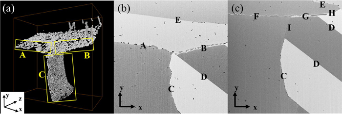
According to the contrast of SEM images of different grain boundaries, two-types of intergranular precipitates with different contrast were present in the volume, ones with dark-gray, and another ones with light-gray. The presences of large number of precipitates were seen at the grain boundaries. In particular, grain boundary A was dominated with dark-gray precipitate, in contrast, two types of precipitates were present at the grain boundary B, major in light-gray precipitates. There was a mixture of dark and light-gray contrast at grain boundary C, where the morphology of precipitates was found very different from others and found only rod-type. Precipitates were then color-coded according to their contrast at the grain boundaries, yellow for dark-gray and green for light-gray precipitates, then seen from various directions as shown in Figs. 14(a), 14(b) and 14(c).

Fig. 14.

A set of images of intergranular precipitates seeing from different orientations. (Online version in color.)

Many of intergranular precipitates were found grown and probably jointed further with other intergranular precipitates due to the additional heat treatment during the tensile test, 1173 K. This is often true for the case of precipitates with light-gray contrast, rather than those having dark-gray contrast, suggesting that the growth rate of light-gray precipitates were higher than that of dark-gray one.

The volume, length, and morphology of these precipitates at each grain boundary are summarized in Table 3 with other grain boundaries.

Table 3. Quantified results of intergranular precipitates at each grain boundaries.

	Grain boundary	A	B	C	D (Twin)	E (Twin)	F	G	H	I (Twin)
Dark gray	Volume (106 nm3)	23.20	8.64	8.78	None	9.32	6.23	23.88	23.68	15.25
	Length (104 nm)	3.98	1.13	16.53		12.11	0.87	2.77	2.71	22.72
	Morphology	Plate	Plate	Rod		Plate, Rod	Plate	Plate	Plate	Plate
Light gray	Volume (106 nm3)	161.83	130.10	59.92	None	19.91	4132.57	73.83	83.55	None
	Length (104 nm)	13.65	24.70	24.35		3.27	19.27	15.34	10.23
	Morphology	Granular	Granular	Rod		Plate	Granular	Granular	Granular

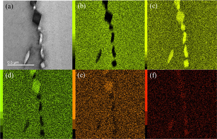
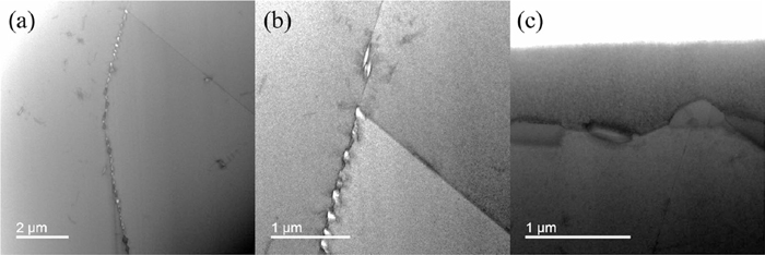
Low-magnified BF-STEM images of grain boundaries are shown in Figs. 15(a), 15(b) and 15(c), where the sizes and morphologies of them are found strongly dependent on the grain boundaries. HAADF-STEM image of grain boundary C was also taken from almost the same region of SEM image, as shown in Figs. 16(a) and 16(b), respectively. By comparing these images, it was somewhat possible to distinguish dark-gray precipitate from light-gray one during HAADF-STEM observation. TEM image and SAED pattern were taken from a dark-gray precipitate of grain boundary C appearing on Figs. 16(a) and 16(b), as shown in Figs. 17(a) and 17(b), respectively. A schematic diagram of Fig. 17(b) is presented on Fig. 17(c). Moreover, similar images were taken from a light-gray precipitate shown in Figs. 17(d) and 17(e), respectively. A schematic diagram of Fig. 17(e) is presented on Fig. 17(f). And Bright-field (BF)-STEM image and a set of elemental distribution maps of Fe, Cr, Ni, Si and N by STEM-EDS analyses, are shown in Figs. 18(a), 18(b), 18(c), 18(d), 18(e), and 18(f), respectively.

Fig. 15.

A set of low magnified bright-field STEM images (a) to (c), where intergranular precipitate’s differences in size and shape depending on grain boundaries are easily seen.

Fig. 16.

A set of (a) HAADF-STEM image and almost the same region of (b) SEM image at grain boundary C.

Fig. 17.

Two sets of BF-TEM image, SAEDP image, schematic diagram of SAEDP from intergranular precipitates at grain boundary C, (a), (b), and (c) as well as (d), (e), and (f).

Fig. 18.

A set of (a) BF-STEM image and EDS elemental distribution map of (b) Fe, (c) Cr, (d) Ni, (e) Si, and (f) N at grain boundary C. (Online version in color.)

These analysis showed that the dark-gray contrast appearing in Fig. 16(b) was determined as Cr₂N and light-gray one as Cr₃Ni₂Si(N). In addition, all of them holds specific crystallographic orientation relationships with matrix, in particular,   

$${\left(111\right)}_{\text{Matrix}}\left|\right|{\left(0001\right)}_{{\text{Cr}}_{\text{2}}\text{N}},{\left[1\overline{1}0\right]}_{\text{Matrix}}\left|\right|{\left[1\overline{1}00\right]}_{{\text{Cr}}_{\text{2}}\text{N}}$$

between Cr₂N and matrix which is the same one for the matrix and the plate-type intragranular Cr₂N, as shown in Fig. 17(c). The presences of cube-cube orientation relationship were confirmed between the matrix and Cr₃Ni₂Si(N), as shown in Fig. 17(f).

4. Conclusion

More than one thousand intragranular and intergranular precipitates in nitrogen added austenitic stainless steel were characterized in detail, were characterized by FIB-SEM, by TEM and by STEM. It was found that there was a variety of morphologies of intragranular dichromium nitride, Cr₂N, precipitates even within the same grains maintaining due to the orientation relationship with the matrix and to the defects surrounding the precipitates. The number density of plate-type precipitate is found larger than that of precipitate with other morphologies, so that the elastic strain energy caused by the misfit-strain might have resulted the formation of different morphologies during the growth. The differences of number densities and orientation relationships, as well as variety of morphologies were statistically understood through current research, namely after characterization of thousands of precipitates from a large volume.

In particular, the Shoji-Nishiyama crystallographic orientation relationship was partially applicable to the case of plate-type Cr₂N precipitate with one of the neighboring matrix as;   

$${\left(111\right)}_{\text{Matrix}}\left|\right|{\left(0001\right)}_{\text{Plate}}\text{, }{\left[1\overline{1}0\right]}_{\text{Matrix}}\left|\right|{\left[1\overline{1}00\right]}_{\text{Plate}}$$

and also for the rod-type Cr₂N precipitate with one of the neighboring matrix as;   

$${\left(111\right)}_{\text{Matrix}}\left|\right|{\left(0001\right)}_{\text{Rod}},{\left[1\overline{1}0\right]}_{\text{Matrix}}\left|\right|{\left[2\overline{1}\overline{1}0\right]}_{\text{Rod}}$$

The Shoji-Nishiyama orientation relationship did not hold at all for the case of granular-type Cr₂N precipitate with one of the neighboring matrix as;   

$${\left(111\right)}_{\text{Matrix}}\left|\right|{\left(11\overline{2}1\right)}_{\text{Granular}},{\left[1\overline{1}0\right]}_{\text{Matrix}}\left|\right|{\left[1\overline{1}00\right]}_{\text{Granular}}$$

In general, two types of intergranular precipitates were observed in the field, and they were determined as Cr₂N and Cr₃Ni₂Si(N) by SAED pattern obtained by TEM, elemental distribution maps via STEM-EDS analysis and direct comparison of SEM and HAADF-STEM images. Although the sizers and morphologies are dependent on the type of grain boundaries, all of them holds specific crystallographic orientation relationships with matrix, such as   

$${\left(111\right)}_{\text{Matrix}}\left|\right|{\left(0001\right)}_{{\text{Cr}}_{\text{2}}\text{N}},{\left[1\overline{1}0\right]}_{\text{Matrix}}\left|\right|{\left[1\overline{1}00\right]}_{{\text{Cr}}_{\text{2}}\text{N}}$$

with Cr₂N, which is the same as the crystallographic relationship between the matrix and the plate-type intragranular Cr₂N precipitate, and also cube-cube relationship with Cr₃Ni₂Si(N).

Furthermore, the formation of a large number of intragranular and intergranular precipitates having various morphologies in nitrogen-added austenitic stainless steel. It was suggested that these variety of intra- and intergranular precipitates should have played crucial roles of high-temperature mechanical strength in nitrogen-added austenitic stainless steel. The strengthening mechanism by precipitates is a future task.

References

• 1)  Corrosion of Austenitic Stainless Steels, Mechanism, Mitigation and Monitoring, Woodhead Publishing Series in Metals and Surface Engineering, eds. by H. S. Khatak and B. Raj, Elsevier, Amsterdam, (2002).
• 2)   A.  Toro,  W. Z.  Misiolek and  A. P.  Tschiptschin: Acta Mater., 51 (2003), 3363.
• 3)   T.  Ogawa,  K.  Suzuki and  T.  Zaizen: Weld. Res. Suppl., 63 (1984), 213.
• 4)   M. F.  McGuire: Stainless Steel for Design Engineers, ASM International, OH, (2008).
• 5)   H.  Bhadeshia and  R.  Honeycombe: Steels: Microstructure and Properties, Butterworth-Heinemann/Elsevier, Amsterdam, (2006).
• 6)   I.  Woo,  M.  Aritoshi and  Y.  Kikuchi: ISIJ Int., 42 (2002), 401.
• 7)   A. F.  Padilha and  P. R.  Rios: ISIJ Int., 42 (2002), 325.
• 8)   R.  Murakami,  Y.  Aoyama,  N.  Tsuchida,  Y.  Harada and  K.  Fukaura: Mater. Sci. Forum, 561–565 (2007), 37.
• 9)   K.  Monma and  H.  Sudo: J. Jpn. Inst. Met., 30 (1966), 558.
• 10)   H.  Suzuki: Sci. Rep. Res. Inst. Tohoku Univ., 4 (1952), 455.
• 11)   I. A.  Yakubtsov,  A.  Ariapour and  D. D.  Perovic: Acta Mater., 47 (1999), 1271.
• 12)   A.  Lehtinen,  F.  Granberg,  L.  Laurson,  K.  Nordlund and  M. J.  Alava: Phys. Rev. E, 93 (2016), 013309.
• 13)   J.  Moon,  S.  Kim,  J.  Jang,  J.  Lee and  C.  Lee: Mater. Sci. Eng. A, 487 (2008), 552.
• 14)   E.  Orowan: Dislocations in Metals, ed. by M. Cohen, AIME, New York, (1954), 69.
• 15)   M. F.  Ashby: Physics of Strength and Plasticity, ed. by A. S. Argon, MIT Press, London, (1969), 113.
• 16)   T.  Hara,  K.  Tsuchiya,  K.  Tsuzaki,  X.  Man,  T.  Asahata and  T.  Uemoto: J. Alloy. Compd., 577 (2013), S717.
• 17)   M.  Oku,  N.  Hiramatsu,  T.  Nagoya and  Y.  Uematsu: Nisshin Steel Tech. Rep., 77 (1998), 47.
• 18)   Y.  Uematsu and  K.  Hoshino: Tetsu-to-Hagané, 69 (1983), 686.
• 19)   Z.  Nishiyama: Materials Science Series, Martensitic Transformation, 1st ed., ed. by M. Fine et al., Academic Press, New York, (1978), 11, 53, 263.