Influence of Microsegregation on the Onset of the Martensitic Transformation

Abstract

Due to the volume change accompanying the fcc to bcc or bct crystal structures in steels, it is a common practice to determine phase transformation temperatures using dilatometry. The martensite start temperature (M_s) is often of particular interest. Experimentally, it is found that the start of the martensite transformation is not indicated by a sharp change in the slope of the dilatation curve as is predicted by the Koistinen – Marburger equation. Rather, there is a gradual change in the slope such that the martensite start temperature is ill-defined. The current work shows that this gradual change in slope can be related to chemical inhomogeneity in the steel caused by interdendritic microsegregation. It is shown that combining the Koistinen – Marburger equation with measured concentration profiles allows experimental dilatation curves to be well predicted.

1. Introduction

Environmental considerations, especially the desire to reduce CO₂ emissions, have led to increased interest in the development of higher strength steels as these allow the design and fabrication of lighter steel structures that require the use of less raw materials and energy for their production.^1,2) In addition, in machine applications, especially in the automotive and transport industries, lightweight structures lead to lower fuel consumption during the use of the steel product. This has led to an increase in the importance of steel microstructures based on either martensite or bainite, due to the high strengths imparted by transformation at low temperature. In the development of such steels, it is desirable to be able to predict the martensite start temperature (M_s) as accurately as possible, either with the aim of avoiding transformation to martensite in order to obtain fully bainitic microstructures, or with the aim of being able to make accurate predictions concerning the austenite to martensite transformation during cooling below M_s. Predicting the development of the martensite volume fraction is of interest, for example, in the case of quenched and partitioned steels, where the amount of austenite remaining at the quench stop temperature is an important parameter in process design.^3,4,5)

For plain iron – carbon alloys, Koistinen and Marburger (K-M)⁶⁾ showed that the transformation of austenite to martensite is well described by the equation   

$$f_a=exp(-\alpha \times (M_s-T_q))$$(1)

where T_q is the quench stop temperature ≤ M_s, α is a material constant and f_a is the fraction of austenite. They also showed that the equation explained the growth of martensite in low-alloyed steels and it has subsequently been widely used to describe athermal martensite formation as a function of temperature below M_s. The form of this equation is such that the martensite transformation rate decreases monotonically from the onset of the transformation at M_s.⁷⁾

Due to the volume change accompanying fcc to bcc or bct crystal structures in steels, it is common practice to determine transformation temperatures, e.g. during continuous cooling, using dilatometry. In the case of the formation of martensite, the K-M equation predicts that the onset of the martensite transformation during cooling should appear as a sharp discontinuous change in the slope of the length – temperature curve away from the thermal contraction of the austenite. If such were the case in practice, the experimental determination of the M_s temperature would be unambiguous. However, very often this is not the case – rather the slope change recorded at the onset of martensite transformation is gradual leading to difficulties in defining the M_s temperature experimentally.^8,9,10,11) In other words, the K-M equation does not predict the experimentally observed sigmoidal shape causing a deviation from the experimental results for the initial 10–15% of the martensite formation.¹²⁾ As a result of this, the offset method has been proposed as a standard way to define M_s.⁸⁾ It has also been proposed that M_s can be determined by fitting a parametric model which calculates strain as a function of temperature during martensitic transformation to experimental dilatation curves.⁹⁾ Sourmail and Smanio⁹⁾ investigated three possible origins for the gradual change in the slope of the length – temperature curve during martensitic formation during dilatometer measurements. They referred to the phenomenon as a “slow-start” for the onset of martensite. Possible origins for the phenomenon were suggested to be solute segregation during solidification, variation in austenite grain size and temperature gradients during thermal treatment of the specimen. They concluded that grain size effects could only explain a minor part of the slow start phenomenon amounting to 4–5°C variations in M_s. The major part of the observed slow-start phenomenon was attributed to temperature gradients in the dilatation specimens arising from the required fast quenching rates. Solute concentration profiles were not measured, but calculated solidification segregation together with the Nehrenberg formula¹³⁾ relating M_s to chemical composition led to the conclusion that solute segregation could only account for about a 4°C spread in M_s towards higher temperatures.

On the basis of experimentally measured solute concentration profiles, this paper shows that chemical inhomogeneity caused by microsegregation actually provides a major contribution to the slow-start phenomenon due to the distribution of M_s temperatures resulting from local variations in chemical composition. Finally, a reformulated closed form of the K-M equation is provided that can be used to predict the effect of chemical inhomogeneity on martensite formation as a function of quench stop temperature.

2. Materials and Methods

The steel with the composition as shown in Table 1 has been studied. It was supplied as an 8 mm thick hot-rolled strip made from a continuously cast slab with a thickness of 167 mm. This is a martensitic stainless steel containing 12 wt.% Cr, known under the Euronorm designation as 1.4003, otherwise known as ASTM 410L. The mean bulk chemical composition shown in the table was determined using electron probe microanalysis (EPMA, Jeol JXA-8200 with a LaB₆ filament), as described in more detail below, and glow discharge optical emission spectroscopy (GDOES, Spectruma GDA 750 Analyzer). The martensitic stainless-steel forms a fully martensitic structure even with air cooling due to its high hardenability.

Table 1. Mean chemical composition of studied steel (wt.% as determined using EPMA).

C	Si	Mn	Cr	Ni
0.044*	0.308	1.078	12.117	0.395

*  Values determined using glow discharge optical emission spectroscopy (Spectruma GDA 750 Analyzer).

Cylindrical specimens of dimensions Ø6×36 mm were cut from the sheet with their axes parallel to the rolling direction. A Gleeble 3800 thermomechanical simulator was used to generate dilatational curves. The specimens were held using sliding jaws which allow free longitudinal expansion and contraction during thermal cycling. The dilatation was measured across the bar thickness at mid-length using quartz contact rods, see Fig. 1. The cylindrical specimens were heated at 10°C/s to 1050°C, held for 2 minutes and then cooled at 48°C/s. The temperatures were recorded with the aid of Type K thermocouples spot-welded to the surface of the specimens at the middle of their length. The Gleeble specimens are heated by an electrical current passing through the specimen from the copper jaws holding the specimen. At the same time, the specimens are cooled by heat flow into the copper jaws, which are cooled by water-cooled aluminium jaw carriers into which they are bolted. After the dilatometry tests, EPMA line scans were made on transverse sections of the solid cylinders cut and polished at the location of the thermocouple. A beam voltage of 15 kV, beam current of 15 nA and beam diameter 10 microns was used together with wavelength dispersive spectrometers configured to detect the elements Al, Cr, Si and Mn. The line scan step size was 10 microns and the dwell time per point was 20 s.

Fig. 1.

Schematic of the cylindrical specimen held with copper jaws on the Gleeble 3800 together with location of the dilatometer quartz rods across the diameter of the specimen. The copper jaws are bolted into water-cooled massive aluminium jaw carriers.

Carbon measurement is problematic with EPMA due to carbon surface contamination from the cracking of residual organic molecules from the vacuum greases, residual oil vapours of the pump equipment and the contamination of the specimen itself.¹⁴⁾ The carbon profile was therefore obtained using Thermo-Calc DICTRA software for one-dimensional diffusion,¹⁵⁾ by assuming an initial uniform concentration and calculating the carbon concentration profile after 2 minutes at 1050°C. As Mn and Cr lowers activity of C, the resultant profile was one where C diffuses into regions where compositions of Mn and Cr are higher.

Due to difficulties in revealing the parent austenite grain structure by etching, the MTEX texture and crystallography analysis toolbox¹⁶⁾ was applied to electron backscatter diffraction (EBSD) results obtained on a Zeiss Sigma field emission scanning electron microscope to reconstruct a parent austenite grain map for the sample following the procedure described by Javaheri et al.¹⁷⁾

With local chemical compositions determined using EPMA, the development of the fraction martensite with temperature and the corresponding theoretical dilatational curves were constructed following the steps below:

1) It is assumed that M_s is linearly related to chemical composition according to the following formula   

$$\begin{array}{l}{\mathrm{M}}_{\mathrm{s}}=a_0+a_C\mathrm{C}+a_{Mn}\mathrm{M}\mathrm{n}+a_{Si}\mathrm{S}\mathrm{i}+a_{Cr}\mathrm{C}\mathrm{r}\\ \hspace{1em}\hspace{0.5em}+a_{Ni}\mathrm{N}\mathrm{i}+a_{Mo}\mathrm{M}\mathrm{o}+a_{Co}\mathrm{C}\mathrm{o}\end{array}$$(2)

where a₀, a_C etc are experimentally determined coefficients available in the literature and the elemental symbols represent the concentrations in wt.%. A number of empirical formulae are available to predict M_s. They are regression equations based on different data sets and ranges of alloying elements as pointed out by Andrews.¹⁸⁾ In the present work, M_s temperatures were calculated using the formulae given in references^{18,19,20,21,22)} to determine which of them best fit with the experimental results. The Kung and Rayment equation¹⁹⁾ was found to be the most suitable for the steel under consideration. This too, is used for steels of similar compositions as described by Miettunen.²³⁾ To obtain a more accurate fit with experiments, a non-linear-least square fitting module from MATLAB was used. The fitting module is implemented after generating theoretical dilatometric curves so as to reduce the difference with the experimental dilatation data. The coefficients of the original Kung and Rayment equation are given in Table 2.

Table 2. Original and final coefficients used in Eq. (2).

Formula	a0	aC	aMn	aSi	aCr	aNi	aMo	aCo
Kung and Rayment	539	−423	−30.4	−7.5	−12.1	−17.7	−7.5	+10
Kung and Rayment (modified)	538	−423	−30.4	−7.5	−6.43	−17.7	−7.5	+10

2) Equation (1) is used to predict the evolution of the martensite fraction for each local composition as a function of temperature below the local M_s temperature using Eq. (2) and the unmodified coefficients in Table 2 together with the initial estimate for α in the K-M equation (0.011).⁶⁾ The overall fraction of martensite in the specimen is then calculated as the sum of the contributions from the 100 analyzed points.

3) Using the above output, specimen dilatation vs temperature plots are constructed based on the non-linear expansion equations for austenite and ferrite as given by Bohemen:²⁴⁾   

$$\frac{\mathrm{\Delta }{D}^{\gamma }}{D_0^{\gamma }}=B_{\gamma }T+B_{\gamma }{\mathrm{\Theta }}_D^{\gamma }\left[exp\left(-\frac{T}{{\mathrm{\Theta }}_D^{\gamma }}\right)-1\right]$$(3)

  

$$\frac{\mathrm{\Delta }{D}^{\alpha }}{D_0^{\gamma }}=\frac{D_0^{\alpha }-D_0^{\gamma }}{D_0^{\gamma }}+B_{\alpha }T+B_{\alpha }{\mathrm{\Theta }}_D^{\alpha }\left[exp\left(-\frac{T}{{\mathrm{\Theta }}_D^{\alpha }}\right)-1\right]$$(4)

where the superscripts and subscripts γ and α refer to the austenite and ferrite phases, respectively, T is absolute temperature, Θ_D is the Debye temperature, B is the thermal expansion coefficient in the high temperature limit, ΔD^γ is the change in diameter for austenite due to thermal expansion above 0 K, $D_0^{\gamma }$ is the theoretical diameter of an austenitic sample at T = 0 K, $D_0^{\alpha }$ is the diameter of the sample with a bcc lattice at T = 0 K, ΔD^α is the difference in diameter between the ferrite at temperature T and austenite at 0 K. The values in Table 3 were found to give the best fit to the data.

Table 3. Coefficients for dilatation model parameters for austenite and ferrite.

	B (K−1)	ΘD (K)
Austenite	23.89e-6	274
Ferrite	18.1e-6	335

4) The change in the diameter of the specimen during transformation from austenite to martensite is calculated as:   

$$D_s=D^{\gamma }+({\mathit{D}}^{\alpha }-{\mathit{D}}^{\gamma })f_m$$(5)

where f_m, the fraction of martensite, is calculated as given in step 2 from the EPMA compositions.

5) The sum of the squares of the differences between the experimentally determined and predicted specimen diameters was determined over the temperature range 385°C to 425°C.

6) Steps 1 to 5 are repeated by modifying the coefficients a₀ and a_Cr in the Kung and Rayment formula, and the factor α in Eq. (1) until the sum of the squares of the differences is minimised. The coefficients of the final modified formulae in given in Table 2. The final value of α was 0.0159 K⁻¹.

3. Results

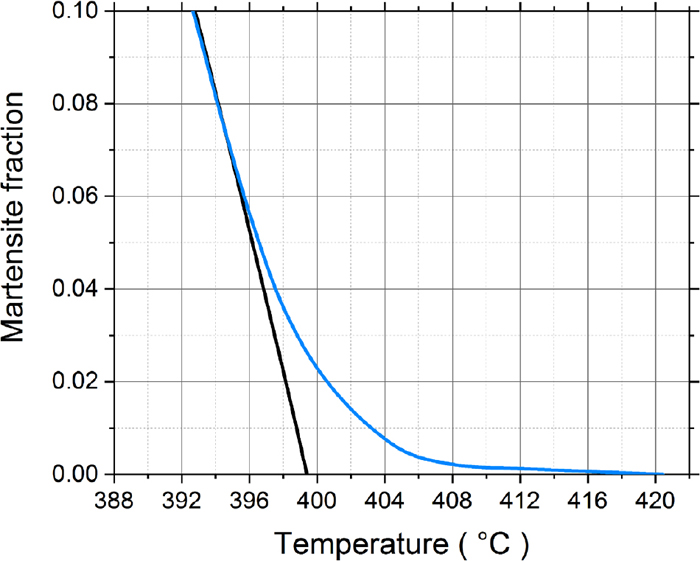
Figure 2 shows examples of the elemental distributions, i.e. for Cr and Mn. The data is more clearly represented in the form of histograms as seen in Fig. 3. Table 4 summarizes the means and the standard deviations for all the EPMA data. The histogram in Fig. 4 show the distribution of the local M_s temperatures calculated from the local chemical compositions using the modified Kung and Rayment formula. The range of calculated M_s temperatures is 30.73°C.

Fig. 2.

Elemental distributions for a) Cr and b) Mn in weight percent. The distributions are measured from 100 points across a distance of 1 mm.

Fig. 3.

Histograms showing variation of Cr (a) and Mn (b) in weight percent.

Table 4. Means and standard deviations of elements in the steel (wt.%).

	Cr	Mn	Si	Ni	C
mean	12.117	1.078	0.308	0.395	0.0440
std.dev.	0.541	0.046	0.025	0.044	0.0017

Cr, Mn, Si, Ni measured using EPMA. C calculated using DICTRA.

Fig. 4.

Frequencies of M_s temperatures calculated using the modified Kung and Rayment formula. Also shown are the means μ and the inhomogeneity parameters a and b as described in the discussion.

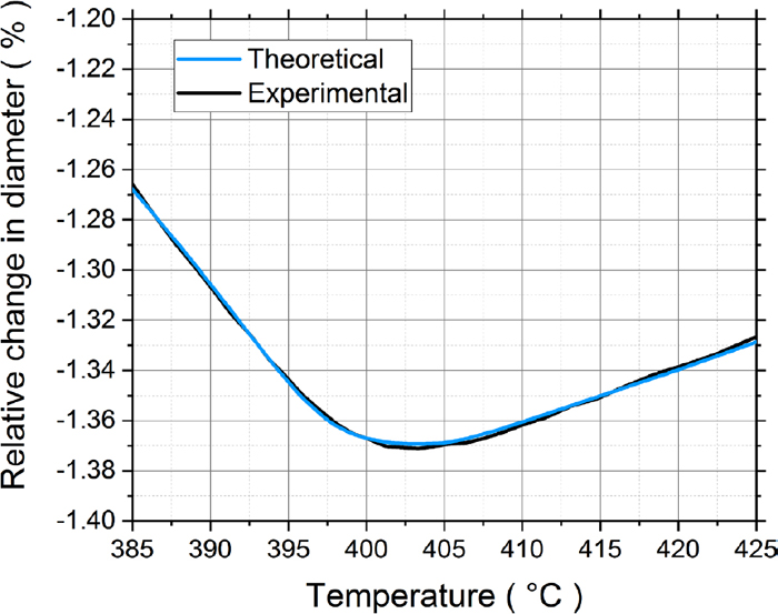
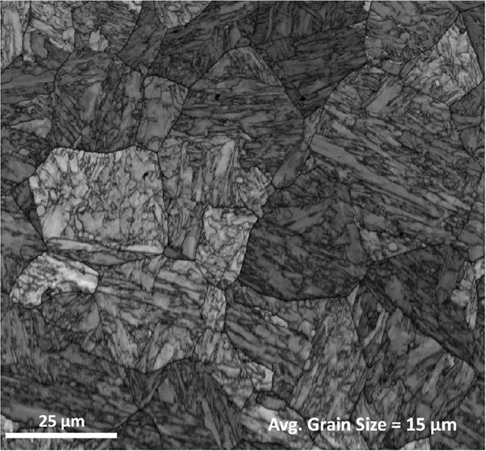
Using the modified Kung and Rayment formula and taking into account the local contents of Si and Mn, the K-M equation was applied to the 100 analysis points and summed to give the overall martensite fraction evolution as shown in Fig. 5. Figure 5 also shows the sharp increase in the martensite fraction as a function of temperature predicted by the K-M equation assuming a homogeneous specimen with the overall mean composition. Compared to that, it can be clearly seen that the onset of martensite formation is gradual with the martensite fraction showing a tail towards higher temperatures than the mean M_s. Using the Bohemen equations Eqs. (3) and (4), a theoretical dilatometric curve was compared with the experimental results during the onset of martensite as seen in Fig. 6. Figure 7 shows the reconstructed prior austenite grain structure of the sample. The grain size was determined using the equivalent circle diameter (ECD) method and the average ECD is given in the figure.

Fig. 5.

Total martensite volume fraction vs. temperature. The blue line is based on the measured 100 local compositions and the black line is based on the mean composition. (Online version in color.)

Fig. 6.

Comparison of the theoretical and experimental dilatometer curves at the onset of martensite. (Online version in color.)

Fig. 7.

Parent austenite grain structure image reconstructed from EBSD data using the Matlab supplemented MTEX toolbox¹⁶⁾ taken from a transverse section of the cylindrical stainless steel specimen. The average grain size is also stated in the image.

4. Discussion

As pointed out by Sourmail and Smanio,⁹⁾ the slow-start could arise as a result of thermal gradients in the dilatometer specimens, which results in cooler regions transforming into martensite earlier than the others during cooling. The dilatometer used in these experiments measures the change in diameter vs. temperature while heat is primarily removed along the axial direction of the cylindrical specimen. The resultant isotherms in the specimens should ideally be parallel to the cylinder diameters giving zero temperature difference between the centre and the surface of the cylindrical specimen. Of course, some heat is lost by radiation to the surrounding vacuum and this results in a temperature gradient in the radial direction. However, calculating the maximum steady state temperature difference between the centre and the surface of the 6 mm diameter cylindrical specimen using the approach described by Semiatin²⁵⁾ revealed that, at temperatures below 440°C, the difference in temperature between the surface and centre due to radiation is less than 0.8°C. Therefore, the temperature gradient in the present case should have a negligible influence on the slow-start phenomenon.

As mentioned above, the empirical formula used to calculate the M_s temperature from the chemical composition of the steel had to be modified to fit with the experimental dilatation curves as seen in Fig. 6. Such an adjustment was to be expected as the Kung and Rayment formula was developed for particular experimental conditions and when they are applied to other conditions, systematic differences are expected. It is known that austenite grain size has an effect on M_s, but this is not explicitly included in the regression equation. Different grain sizes can therefore be expected to influence the magnitude of the constant a₀ in the regression formula. Yang and Bhadeshia²⁶⁾ show that M_s temperatures increases with an increase in the austenitic grain size. The average ECD was found to be about 15 μm with a standard deviation of about 8 μm. The maximum ECD was found to be about 37 μm. Of course, the variation in the size of individual parent austenite grains may create scatter in local Ms temperatures, but as pointed out by Sourmail and Smanio⁹⁾ this can only account for 4–5°C of the slow start, but not the full 30.74°C range of the slow start. Looking at the products of the Kung and Rayment regression coefficients in Table 2 and the standard deviations of the chemical contents in Table 4, it can be seen that the effect of variations in Cr will account for most of the slow start phenomenon, being about 5 times higher than the next most significant element Mn. Therefore, errors in the regression coefficients for C, Mn, Si and Ni will not significantly affect the magnitude of the slow start, i.e. the relative positions of the M_s temperatures on the temperature scale. However, they will affect the absolute values of the Ms temperatures. Our approach of only considering possible errors in the coefficients a₀ and a_Cr is therefore justified: the modified value for a₀ will account for possible errors in a₀, a_C, a_Mn, a_Si, a_Ni, and a_Mo as far as the absolute values of the M_s temperatures are concerned while the modified value of a_Cr makes the predicted slow start better fit the observed. The difference between the original and modified values of a₀ is, in fact, only 1°C. As discussed above, the difference includes effects of grain size and errors in the regression coefficients of the alloying elements other than Cr. The fitting procedure used resulted in a modified absolute value for a_Cr that was smaller in magnitude than the original Kung and Rayment value, i.e. −6.43 as opposed to −12.1. This means that the slow start can be well explained by the observed variations in Cr content: keeping the original value for a_Cr would have predicted an even slower start to the martensite transformation.

The amplitude of the interdendritic microsegregation concentration profiles present after solidification is reduced during cooling of the cast material²⁷⁾ and subsequent reheating prior to rolling,²⁸⁾ but, as shown by the results of the EPMA scans of Fig. 2, marked differences remain in the finished plates despite overall rolling reductions of approximately 14 times. In the steel studied, the regions with the leanest local chemical composition caused the highest calculated M_s temperatures to be more than 20°C above the mean, which can be seen as well explaining the earlier slow start of the martensite transformation. The lean alloyed regions can be expected to transform into martensite first after which the other regions contribute to the ever-increasing martensite fraction as shown in Fig. 5. The results seen in Fig. 5 are similar to those of Bohemen and Sietsma¹¹⁾ where the theoretical M_s temperature is somewhat lower than the M_s observed experimentally, where there is a gradual onset during martensite transformation.

Figure 5 also shows that the lean-alloyed regions affect the martensite fraction mainly over the first 10% of the transformation. As the martensitic transformation proceeds further, the evolution of the martensite fraction calculated using the K-M equation from the averages of the 100 measured local compositions and the fully homogenised steel composition follow the same general trend.

With the theoretical curves serving as good approximations to the experimental curves, we can make good quantitative predictions of the M_s temperatures. The gradual slope change during the onset of the martensitic transformation can be related to the dispersion of M_s temperatures due to local compositional variation.

A closed-form equation which includes the gradual start during the onset of martensite evolution would be useful as it could be readily implemented in simulation software such as those based on finite element analyses like Abaqus FEA. Therefore, to describe the gradual onset of martensite evolution, the existing K-M equation needs to be reformulated to take into account the inhomogeneities in chemical composition. This can be achieved as follows.

The K-M equation, Eq. (1), may be rewritten for the fraction of martensite f_m in the form of piecewise function:   

$$f_m(T_q,M_s)=\{\begin{array}{cc}1-exp(-\alpha (M_s-T_q)),& T_q\le M_s\\ 0,& T_q>M_s\end{array}$$(6)

As seen in Fig. 4, M_s is a random variable which can be described with a probability density function p(M_s). Further, the expectation value of martensite fraction f_m depending on temperature T_q and probability density function p(M_s) can be written as:   

$$⟨f_m\left(T_q,p(M_s)\right)⟩={\int }_{-\infty }^{\infty }p(M_s)f_{m}d{M}_s$$(7)

Equation (7) can then be numerically integrated to find f_m for any T_q, if the distribution of M_s is described with the probability density function p(M_s). For a given steel, such functions can be determined experimentally, as described above.

The practical implementation of Eq. (7) would be simplified if the equation could be presented in a closed form, thereby allowing a simple evaluation of the slow start phenomenon dependent on the degree of steel inhomogeneity. Quantitatively, such an inhomogeneity has to be described in terms of scalar parameters, like the mean value μ and variance σ² of the random variable M_s.

To find a solution in a closed form, let us assume that p(M_s) can be approximated with a uniform probability density function p_u(M_s) defined as the following piecewise function:   

$$p_u(M_s)=\{\begin{array}{c}0,\hspace{1em}\hspace{1em}{M}_s<a\\ {\displaystyle \frac{1}{b-a}},\hspace{1em}a\le M_s\le b\\ 0,\hspace{1em}\hspace{1em}{M}_s>b\end{array}$$(8)

where a and b describe the lowest and the highest M_s in the assumed uniform distribution. The exact values of a and b providing a close approximation to the actual general distribution p(M_s) will be defined later in this section. Substituting p_u(M_s) into Eq. (7) and taking into account the piecewise functions defined in Eqs. (6) and (8), the general Eq. (7) can be rewritten as:   

$$⟨f_m(T_q,a,b)⟩=\{\begin{array}{c}{\int }_T^b{\displaystyle \frac{1}{b-a}}\left(1-exp\left(-\alpha (M_s-T_q)\right)\right)d{M}_s,\mathrm{\hspace{0.17em} }\mathrm{\hspace{0.17em} }a\le T\le b\\ {\int }_a^b{\displaystyle \frac{1}{b-a}}\left(1-exp\left(-\alpha (M_s-T_q)\right)\right)d{M}_s,\mathrm{\hspace{0.17em} }\mathrm{\hspace{0.17em} }T<a\end{array}$$(9)

Equation (9) can be solved in a closed form:   

$$⟨f_m(T_q,a,b)⟩=\{\begin{array}{c}{\displaystyle \frac{\alpha (b-T_q)-\left(1-exp\left(-\alpha (b-T_q)\right)\right)}{\alpha (b-a)}},\mathrm{\hspace{0.17em} }\mathrm{\hspace{0.17em} }a\le T\le b\\ 1+{\displaystyle \frac{exp\left(-\alpha (b-T_q)\right)-exp\left(-\alpha (a-T_q)\right)}{\alpha (b-a)}},\mathrm{\hspace{0.17em} }\mathrm{\hspace{0.17em} }T<a\end{array}$$(10)

or in terms of K-M kinetics f_m(T_q, M_s) described in Eq. (6):   

$$⟨f_m(T_q,a,b)⟩=\{\begin{array}{c}{\displaystyle \frac{\alpha (b-T_q)-f_m(T_q,b)}{\alpha (b-a)}},\hspace{1em}a\le T\le b\\ 1+{\displaystyle \frac{f_m(T_q,a)-f_m(T_q,b)}{\alpha (b-a)}},\hspace{1em}T<a\end{array}$$(11)

The values of the parameters in the uniform probability density function p_u(M_s) a and b that provide a close approximation of the general distribution p(M_s) can be found using the moments matching principle. This states that as many moments as possible have to be matched to provide the best possible approximation. In the case of the uniform distribution, the first and second central moments, i.e. the mean and variance, can be matched. As the mean and variance for p_u(M_s) are defined as μ = (b−a)/2 and σ² = (b−a)²/12, a and b can be written as:   

$$\begin{array}{l}a=\mu -\sqrt{3}\sigma \\ b=\mu +\sqrt{3}\sigma \end{array}$$

and Eq. (11) can be rewritten as:   

$$\begin{array}{l}⟨f_m(T_q,\mu ,\sigma )⟩=\\ \{\begin{array}{c}{\displaystyle \frac{\alpha (\mu +\sqrt{3}\sigma -T_q)-f_m(T_q,\mu +\sqrt{3}\sigma )}{2\sqrt{3}\sigma \alpha }},\mathrm{\hspace{0.17em} }\mathrm{\hspace{0.17em} }\mu -\sqrt{3}\sigma \le T\le \mu +\sqrt{3}\sigma \\ 1+{\displaystyle \frac{f_m(T_q,\mu -\sqrt{3}\sigma )-f_m(T_q,\mu +\sqrt{3}\sigma )}{2\sqrt{3}\sigma \alpha }},\mathrm{\hspace{0.17em} }\mathrm{\hspace{0.17em} }T<\mu -\sqrt{3}\sigma \end{array}\end{array}$$(12)

μ and σ can be determined from experimental or theoretical concentration profiles and substituted directly in Eq. (12) to find the martensite fraction for any temperature T_q. A comparison of Eq. (12), with the results of a full numerical integration of the distributions in Fig. 4 and the use of the Koistinen-Marburger equation based on the mean composition is shown in Fig. 8.

Fig. 8.

Evaluation of slow start phenomenon: comparison of the analytical formula, numerical integration and Koistinen-Marburger kinetics for 12Cr steel. The parameters a and b are from Table 5. (Online version in color.)

Table 5. Inhomogeneity parameters [°C] describing the spread in M_s.

μ	σ	a	b	b−a	b−μ
399.41	5.40	391.44	407.36	15.92	7.95

From Fig. 8, it is clear that there is a discrepancy between the numerical integration of the martensite evolution based on the actual 100 EPMA compositions and the martensite evolution calculated from the proposed formula Eq. (12). This is because the proposed formulation assumes that the M_s temperatures are uniformly distributed between the upper and lower limits b and a, while experimentally the M_s temperatures follow a more complex distribution as show in Fig. 4.

5. Conclusion

This paper has explored the extent to which the dispersion of M_s temperatures arising from local chemical inhomogeneity can explain the slow start to the martensite transformation commonly observed in dilatometer measurements. Chemical inhomogeneity originates from the microsegregation of alloying elements during dendritic solidification. During cooling, the chemically lean regions have a relatively high M_s temperature and transform into martensite earlier than other regions.

A cylindrical martensitic stainless steel sample was austenitized and cooled to room temperatures at 48°C/s using a Gleeble thermomechanical simulator equipped with a dilatometer. The chemical inhomogeneity of the steel was quantified by measuring the compositions from 100 equally spaced points across 1 mm distance on a transverse section using EPMA. The M_s temperatures were calculated for all these 100 points and the average martensite fractions as a function of temperature were calculated using the Koistinen-Marburger equation. This resulted in a gradual start during the onset of the martensite transformation as opposed to the sharp onset predicted for a homogeneous composition equal to the mean composition of the steel. The predicted dilatation curve fitted the observed experimental curve well, showing that the chemical inhomogeneity can completely explain the gradual start during the onset of martensite transformation.

Taking the chemical inhomogeneity into consideration, the K-M equation was reformulated into a closed-form solution so as to predict a gradual slow-start during the onset of martensite transformation for use e.g. in finite element method modelling. The closed-form solution allows for straightforward calculation of martensite evolution with an assumption that the M_s temperatures are uniformly distributed between upper and lower values that can be calculated from the M_s value for the mean composition and the standard deviation of the local M_s values.

Acknowledgements

The authors are grateful for financial support from the European Commission under grant number 675715 – MIMESIS – H2020-MSCA-ITN-2015, which is a part of the Marie Sklodowska-Curie Innovative Training Networks European Industrial Doctorate Programme. The authors would like to thank Juha Uusitalo and Dr Mahesh Somani from the University of Oulu for their support with regards to the dilatometry experiments. The authors thank Vahid Javaheri for his support in the parent austenite grain reconstruction from EBSD images. The authors also thank Leena Palmu for her support with the EPMA measurements. The authors would also like to thank Dr Pasi Suikkanen from SSAB Europe Oy for his support. The support of Outokumpu Oyj in providing the steel studied is also acknowledged.

References

• 1)   J.  Kömi,  P.  Karjalainen and  D.  Porter: Encyclopedia of Iron, Steel, and Their Alloys, CRC Press, Boca Raton, FL, (2016), 1109.
• 2)   D.  Van Pham,  J.  Kobayashi and  K.-I.  Sugimoto: ISIJ Int., 54 (2014), 1943.
• 3)   A. J.  Clarke,  J. G.  Speer,  M. K.  Miller,  R. E.  Hackenberg,  D. V.  Edmonds,  D. K.  Matlock,  F. C.  Rizzo,  K. D.  Clarke and  E.  De Moor: Acta Mater., 56 (2008), 16.
• 4)   E.  De Moor,  J. G.  Speer,  D. K.  Matlock,  J. H.  Kwak and  S. B.  Lee: ISIJ Int., 51 (2011), 137.
• 5)   G. A.  Thomas,  F.  Danoix,  J. G.  Speer,  S. W.  Thompson and  F.  Cuvilly: ISIJ Int., 54 (2014), 2900.
• 6)   D. P.  Koistinen and  R. E.  Marburger: Acta Metall., 7 (1959), 59.
• 7)   D.  Ivanov and  L.  Markegård: HTM J. Heat Treat. Mater., 71 (2016), 99.
• 8)   H. S.  Yang and  H. K. D. H.  Bhadeshia: Mater. Sci. Technol., 23 (2007), 556.
• 9)   T.  Sourmail and  V.  Smanio: Mater. Sci. Technol., 29 (2013), 883.
• 10)   A.  Kamyabi-Gol,  D.  Herath and  P. F.  Mendez: Can. Metall. Q., 56 (2017), 85.
• 11)   S. M. C.  van Bohemen and  J.  Sietsma: Mater. Sci. Technol., 25 (2009), 1009.
• 12)   F.  Huyan,  P.  Hedström and  A.  Borgenstam: Mater. Today: Proc., 2 (2015), S561.
• 13)   A. E.  Nehrenberg: Trans. AIME, 167 (1945), 494.
• 14)   F.  Robaut,  A.  Crisci,  M.  Durand-Charre and  D.  Jouanne: Microsc. Microanal., 12 (2006), 331.
• 15)   A.  Borgenstam,  L.  Höglund,  J.  Ågren and  A.  Engström: J. Phase Equilib., 21 (2000), 269.
• 16)   T.  Nyyssönen,  M.  Isakov,  P.  Peura and  V. T.  Kuokkala: Metall. Mater. Trans. A, 47 (2016), 2587.
• 17)   V.  Javaheri,  N.  Khodaie,  A.  Kaijalainen and  D.  Porter: Mater. Charact., 142 (2018), 295.
• 18)   K. W.  Andrews: J. Iron Steel Inst., 203 (1965), 721.
• 19)   C. Y.  Kung and  J. J.  Rayment: Metall. Mater. Trans. A, 13 (1982), 328.
• 20)   P.  Payson and  C. H.  Savage: Trans. Am. Soc. Met., 33 (1944), 261.
• 21)   R. A.  Grange and  H. M.  Stewart: Trans. AIME, 167 (1946), 467.
• 22)   W.  Steven: J. Iron Steel Inst., 203 (1956), 349.
• 23)   I.  Miettunen,  S.  Anttila,  T.  Kaupinmäki and  D. A.  Porter: 5th Int. Conf. on ThermoMechanical Processing (TMP), Associazione Italiana di Metallurgia, Milan, (2016), 5069.
• 24)   S. M. C.  Van Bohemen: Scr. Mater., 69 (2013), 315.
• 25)   S. L.  Semiatin,  D. W.  Mahaffey,  N. C.  Levkulich and  O. N.  Senkov: Metall. Mater. Trans. A, 48 (2017), 5357.
• 26)   H. S.  Yang and  H. K. D. H.  Bhadeshia: Scr. Mater., 60 (2009), 493.
• 27)   Y.  Huang,  M.  Long,  P.  Liu,  D.  Chen,  H.  Chen,  L.  Gui,  T.  Liu and  S.  Yu: Metall. Mater. Trans. B, 48 (2017), 2504.
• 28)   H. E.  Lippard,  C. E.  Campbell,  V. P.  Dravid,  G. B.  Olson,  T.  Björklind,  U.  Borggren and  P.  Kellgren: Metall. Mater. Trans. B, 29 (1998), 205.