Abstract
Fluid flow of liquid steel in a slab mold influenced by three different submerged entry nozzles with the same bore sizes but different ports including rectangular, square, and round shape at immersion depth of 185 mm was studied. The analysis includes numerical simulations and physical modeling. The results show that the port shape has great effects over the fluid dynamics of the liquid steel inside the slab mold. The comparison among the three nozzle port designs indicates that the nozzle with square ports, (SEN-S), decrease the jets velocity, promote a symmetrical path inside the mold and decrease the bath level oscillations; representing the best choice to control the turbulence and decrease the quality problems.
1. Introduction
Fluid flow in continuous casting molds is important because it governs production rate of the caster and quality of the product. However, both aspects have opposite consequences. On one side, to get high production rate it is necessary, to increase the casting speed; on the other side, an increase of casting speed leads to flux entrapment to form inclusions impairing the product quality. This opposite relationship between production and quality has been the driving force of many research reports related to fluid flow of liquid steel, particularly in slab molds.1,2,3,4) The fluid flow inside the casting mold is characterized by having a turbulent behavior, which is associated with risky possibilities such as shell-thinning breakout, formation of slivers and inclusion entrapment.5,6,7,8) The turbulence intensity in the mold depends on the submerged entry nozzle, (SEN), port design, the casting speed and the SEN immersion depth. To reach both productivity and quality, it is necessary to understand the effect that the SEN ports have on the unsteady flow structures in this process. Unfortunately, due to the high temperature of steel, it is difficult to perform velocity measurements directly in molten steel.9) Physical models and mathematical simulations are alternative ways to study the behavior of liquid steel inside the mold. Previous approaches are of great help in diagnosing and understanding the phenomena that dominate the behavior of the process, which provides the basis for achieving optimization that has an impact on minimization of production costs. The aim of this work was to assess the unsteady flow structures into the slab mold developed by the SEN-R (current nozzle), SEN-S and SEN-C for the same operating conditions (see Table 1). The comparison among the three SEN port designs was carried out through physical experiments and numerical simulations.
Table 1. Operating conditions used in the Physical experiments and computational simulations.
| Parameter | Value |
|---|
| PHYSICAL MODEL |
| Casting Speed, (m/min), (m/s) | 0.9, 0.015 |
| Equivalent flow rate, (m3/s) × 103 | 6.4 |
| Slab mold size, (m3) | 1.88 × 0.23 × 0.7 |
| Air zone, (m) | 0.1 |
| Nozzle immersion*, (m) | 0.185 |
| NUMERICAL MODEL |
| Casting Speed, (m/s) | 0.015 |
| Pressure inlet, (Pa) | 101325 |
| Nozzle immersion*, (m) | 0.185 |
| Viscosity of the liquid steel, (Pa s) | 0.0064 |
| Kinematic viscosity of the steel, (m2/s) | 1×10⁻⁶ |
| Density of the liquid steel, (kg/m3) | 7100 |
| Viscosity of the air, (Pa s) | 1.7894×10⁻⁵ |
| Density of the air, (kg/m3) | 1.225 |
| Interfacial tension between air and steel, (N/m) | 1.6 |
| Turbulence Model | LES |
| Interfacial model | VOF |
| Pressure-velocity couple | SIMPLEC |
| Convergence criterion | Less than 10−4 |
| *Distance from the free surface to the upper exit port position |
2. Presentation of the Case
Recently, a company that produces peritectic steels, acquired a new SEN design with rectangular ports, with10-degree upward ports angle, which is presented in Fig. 1(a). This nozzle was designed to create greater stirring into the mold and send fresh steel toward the upper mold corners to cast crack sensitive steels. Nevertheless, recent reports indicate that the current nozzle (SEN-R) promotes excessive turbulence at bath level when its maximum immersion depth is 185 mm (to use the complete zirconia band), entraining particles from mold flux, slivers, and even breakout problems.10) To solve these quality and operational problems, the plant is considering two alternative SEN port designs to replace the actual nozzle; the first has square ports (SEN-S), and the second has round ports (SEN-C). The shape and dimensions of these nozzles are shown in Figs. 1(b) and 1(c), respectively. Both proposed designs have a port size greater than the actual nozzle (SEN-R), looking for jet velocity reduction and consequently to decrease the turbulence inside the mold without compromising productivity and quality. In other words, looking for a good symmetric flows and suitable stirring conditions to melt the mold flux and maintaining small meniscus disturbances by oscillation waves, and vortex flows.11)

3. Water Model
A full-scale water model of the slab mold was built with transparent plastic plates with total height of 1700 mm. To recreate the fluid flow of liquid steel into the mold, the model was partially inserted (250 mm) into a pit full of water to represent the continuity of the strand. The pit contains a submergible water pump to transport water through a vertical pipe, which has a flow meter and a precision valve embedded along the line to control the flow rate of water fed into the model. This pipe line feeds the tundish fixing the bath height at the same level (1 m) as in the actual tundish in the plant. This configuration permits the water to be recycled. The flow rate from the tundish to the mold was controlled through a stopper rod as the actual system at the plant. The physical model includes the three full scale plastic prototypes of the real SEN designs used at the plant. A detail explanation of the experimental setup can be found in reference 10. The experimental techniques employed to study the fluid flow in the mold are described in the next lines.
3.1. Particle Image Velocimetry (PIV), Dye Injection and Ultrasonic Sensors
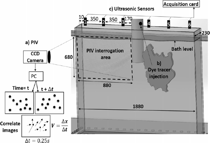
To measure flow velocities in the water model, the PIV technique was employed. The principle of PIV is to determinate the flow velocities by measuring the displacement vector of illuminated particle images during a known time interval. In this work, particles with diameters of approximately 20 μm and density of 1020 kg/m3 were seeded into the fluid prior to the measurements.12) A 1 mm thick laser sheet was displayed in the central plane, at half the mold thickness. The displacements of particles were recorded with a CCD camera (DANTEC-Double Image 700) and the signals were converted to velocity magnitudes and validated through a Fast Fourier Transforms algorithm. The studied area involves the upper-half side of the mold with a size of 880 × 660 mm2 as shown in Fig. 2(a). To reveal the flow pattern as a function of the nozzle port shape, a red dye tracer was injected as a pulse through an orifice located in the upper side of the SEN, Fig. 2(b). The mixing kinematics of the dye was recorded using a conventional video-camera, which was fixed in front of the water model. Finally, the bath level in the mold was monitored in real time using six ultrasonic sensors. Three were placed at each side of the SEN; one close to the narrow mold wall (1 and 6), another at the midpoint between the SEN and narrow mold wall (sensor 2 and 5) and the last one, close to the SEN body (sensor 3 and 4). Figure 2(c) shows a schematic of the ultrasonic sensors location. The ultrasonic signals were converted into digital data using an acquisition card.13) Digital data were received by a plotter system to visualize bath level oscillations during the experimental work and were recorded for further analysis.
4. Mathematical Model
The developed model is based on the solution of the Navier-Stokes equations for incompressible viscous flow, together with the multiphase model (Volume Of Fluid or VOF), and the turbulence model (Large Eddy Simulation or LES), which are embedded in the CFD (Computational Fluid Dynamics) commercial software ANSYS FLUENT®. The inlet velocity is calculated to maintain the desired casting speed at the outlet. To solve the mathematical model, the next assumptions were considered:14) a) the fluid flowing into the mold was assumed to have Newtonian behavior, b) a pressure inlet condition is applied at the mold top (p = 101325 Pa) to model the effects of a system open to the atmosphere, c) the system was modeled considering unsteady state and isothermal conditions, consequently the thermos-physical properties remain constant, d) non-slip conditions were applied at all solid surfaces, and e) convergence criterion was obtained when the residuals of the output variables reached values equal or smaller than 1×10⁻⁴.
4.1. The Turbulence Model (LES)
In this study the LES model was employed to simulate the flows. In this model the large length scale, three-dimensional (3D), and unsteady turbulent motion are directly resolved, whereas the effects of the smaller scale motions are modeled. Therefore, the large eddies are mathematically filtered and the dissipative small-scale eddies are modeled to get closure of the motion equations. The filtering is represented using an SGS k model.15,16) The governing equations for the resolved flow field account for conservation of mass and momentum as:17)
|
D
v
i
Dt
=-
1
ρ
∂p
∂
x
i
+
∂
∂
x
j
v
eff
(
∂
v
i
∂
x
j
+
∂
v
j
∂
x
i
)
| (2) |
Where, the subscripts i and j represent the three Cartesian directions and repeated subscripts imply summation. The symbols p and vi in Eqs. (1) and (2) represent the pressure and filtered velocities. The residual stresses, which arise from the unresolved small eddies, are modeled using an eddy viscosity (vt). The SGS kinetic energy (SGS k) model employed here requires solving the following additional transport equation, which includes advection, production, dissipation, and viscous diffusion.18,19)
|
∂
k
sgs
∂t
+
v
i
∂
k
sgs
∂
x
i
=
v
t
|
S
˜
|
2
-
C
ε
k
sgs
3
2
Δ
+
∂
∂
x
i
(
v
0
+2
v
t
∂
k
sgs
∂
x
i
)
| (4) |
Where Δ is the filtration volume and Δi is the size of the computational cell:
|
Δ=
(
Δ
x
Δ
y
Δ
z
)
1
3
| (5) |
|
v
t
=
C
l
Δ
k
sgs
3
2
| (6) |
where
|
S
˜
|
is the magnitude of the strain-rate tensor, defined as:
|
|
S
˜
|=
2
S
˜
ij
S
˜
ij
| (7) |
|
S
˜
ij
=
1
2
(
∂
v
i
∂
x
j
+
∂
v
j
∂
x
i
)
| (8) |
The parameters Cε = 1.0 and Cl = 1.0 can be treated as constants.15)
4.2. Multiphase Model
To model the interface between air and steel, the Volume of Fluid (VOF) model20,21) was used. This model is a Eulerian method that uses a volume fraction indicator to determine the location of the interfaces of different phases in all cells of a computational domain. In order to minimize the effects of the inaccurate interpolation for some physical quantities, the model needs equations accounting for the variation of density as well as a viscosity. If it is considered incompressible, immiscible fluids, (no phase change between fluids), then the variable density and viscosity present at each cell can be expressed on the base of their fraction as shown below:
|
ρ
mix
=
α
ρ
ρ
ρ
+(
1-
α
q
)
ρ
ρ
| (9) |
|
μ
mix
=
α
ρ
μ
ρ
+(
1-
α
q
)
μ
ρ
| (10) |
A unique continuity equation for the transient system is derived depending on the number of phases. Therefore, the Eq. (11) is divided by the number of phases q in the cell. Mass exchange between phases can be modeled by introducing an additional source term Sαq.
|
1
ρ
q
[
∂
∂t
(
α
q
ρ
q
)
+∇⋅(
α
q
ρ
q
v
→
)
=
S
αq
+
∑
p=1
n
(
m
˙
pq
-
m
˙
qp
)
]
| (11) |
The mass transfer from phase p to phase q and from phase q to phase p is given by the right side of the equation, where Sαq is a source term. The volume fraction equation for the secondary phase (air) is solved through Eq. (11); the volume fraction of the primary phase is computed using the following constraint:
The volume fraction Eq. (11) is solved through an explicit time discretization method. The standard finite-difference interpolation schemes are applied to the volume fraction values that were computed at the previous time step.
|
α
q
n+1
ρ
q
n+1
-
α
q
n
ρ
q
n
Δt
V+
∑
f
(
ρ
q
U
f
n
α
q⋅f
n
)
=[
S
αq
+
∑
p=1
n
(
m
˙
pq
-
m
˙
qp
]V
| (13) |
A single set of momentum equations is solved throughout the domain, and the resulting velocity fields is shared among the phases. The momentum equation, shown below, is dependent on the volume fraction of all phases through properties ρ and μ.
|
∂
∂t
(
ρ
mix
v
→
)
+∇⋅(
ρ
mix
v
→
v
→
)
=-
∇
p
+∇[
μ
mix
(
∇
v
→
+∇
u
→
)
]+ρg+
S
σ
| (14) |
The last term of this equation is a momentum source related with balance or forces arising by surface tension properties. The surface tension value was considered constant along the interface between the phases and it is treated as a source term in the momentum equation.
4.3. Numerical Procedure
The governing equations were discretized using the finite volume technique and solved considering the computational segregated-iterative method. The non-linear momentum equations were linearized using the implicit approach. The discretization was performed using the Second Order Upwind scheme. The PRESTO22) scheme was used for pressure interpolation. The algorithm SIMPLEC22) was used to couple the pressure-velocity variables. To model the flow of two immiscible phases the VOF model is the most appropriated. The computational mesh consists of 1300000 structured cells. The total computing simulation time was of 300 s and the time step was maintained at 0.01 s.
5. Results
The ideal flow pattern is called a double roll flow (DRF). Which must be permit a gentle roll flow along to meniscus, transporting steel in contact with the molten flux to provide even the ideal solidifications conditions and another downwards roll-flow. To reach this behavior the symmetry of the flow and the turbulence intensity inside the mold, must be controlled.
5.1. Flow Symmetry
For the first stage of this study, images from the red dye injection experiments, (two different instants) were selected to compare the performance of the three SEN port designs. The first image corresponds at the instant when the jet reaches the narrow mold face, and the second one is when the double roll pattern is revealed by the tracer. Figure 3(a) shows that the SEN-R yields a pair of asymmetrical jets with different velocity and impact depth between left and right side. This behavior promotes high flow asymmetry when the jets split at the narrow mold face into upward and downward streams, as can be seen in Fig. 3(b). Figure 3(c) shows that the SEN-S develop a pair of symmetrical jets that impact at the same depth and at the same time, which is translated in a good behavior, Fig. 3(d). Meanwhile, the Fig. 3(e) shows that the SEN-C develops a pair of straight jets whit tiny difference in impact depth between left and right side. Which is the cause of slightly asymmetric flow pattern as can be seen in Fig. 3(f).
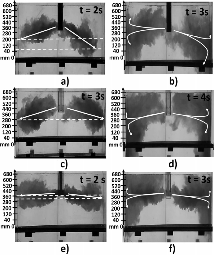
The averaged values of the depth impact points of the left and right jet for each SEN design are plotted in Fig. 4. It is clear that the SEN-R is the worst case in terms of symmetry, even though this nozzle has ports with an upward angle, aiming to send hot flow at the upper mold corners; the actual behavior is completely opposite to the objective for which it was designed; in addition, the difference between the left and right jet is large and the flow symmetry is affected.
5.2. General Flow Patterns
Instant velocity fields measured with the PIV technique were selected to study the flow pattern observed on the dye injection experiments. The investigation area is the upper central frontal plane in the left side of the mold.
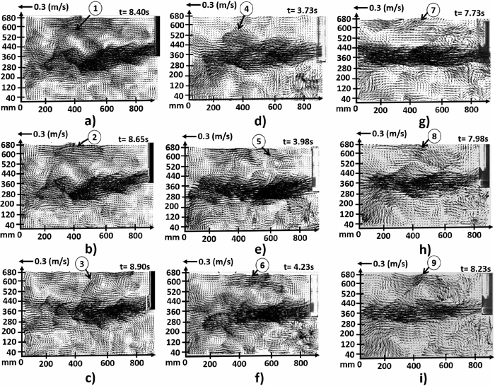
Figure 5, shows three consecutive transitory images (with a time difference of 0.25 s between each figure), for the three SEN port designs. The SEN-R, presented in Figs. 5(a)–5(c), develops a jet that does not conserve an integral shape; instead, yields wandering motions of the jets and part of the jet is detached toward the bath surface marked by numbers “1” and “2”. Other detached flow can transport great volumes of fluid affecting the meniscus stability as indicated by the number “3”. The twisting effects show the dynamic and changing nature of the flow pattern developed by the current nozzle in the plant. Figures 5(d)–5(f) correspond to the flow pattern developed by the SEN-S. Detached flows from the jet are observed (marked with the numbers “4”, “5” and “6”) but with less intensity in comparison to the SEN-R. The flow patterns presented in Fig. 5(g)–5(i) corresponding to the SEN-C, are quite different from those described for the SEN-R and SEN-S. The jet maintains its shape from the nozzle port to the impinging point on the narrow face of the mold. The straight jet does not suffer detaching flows. However, the jets promote that the upper roll flows acquire high velocity at the bath level as is indicated by the numbers “7”, “8” and “9”.
Comparison of the experimental measurements of velocity using the PIV and the mathematical simulations using the LES model are shown in Fig. 6. Instantaneous images for each nozzle were selected and then compared to corroborate with the experimental results. As shown, there is a good agreement between the measurements and simulations results.
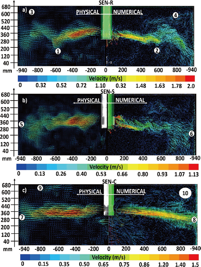
The Fig. 6(a) shows that the SEN-R yields downward meandering jets that lose the integrity of their shapes at a distance of 600 mm approximately, (market with the numbers “1” and “2”). The velocities in the center of the jet emerging from the nozzle ports are 2 m/s and 1.78 m/s from PIV measurements and from numerical approach, respectively. Although the jets emerge with a negative angle, the formation of the upper recirculation causes high velocities near the bath level zone, as indicated by the numbers “3” and “4”. The SEN-S, shown in Fig. 6(b), develops a pair of jets with output speeds of 1 m/s and 0.95 m/s from the experimental and numerical results, respectively. The jets lose speed along their path to the narrow mold wall, where the impact velocities are 0.1 to 0.13 m/s; (marked by the numbers “5” and “6”) from experimental and numerical results, respectively. The jet meanders with less intensity than the jet of the SEN-R. Lastly, the SEN-C presented in the Fig. 6(c) develops straight jets that conserve their shape along its path to the narrow mold face, where they split in upward and downward streams, forming the double roll pattern. These jets, impact the narrow face of the mold with larger velocities (0.5 m/s and 0.65 m/s from experimental and numerical approaches, respectively) with probable shell washing effects (market by the numbers “7” and “8”) and shear flows at bath level, as is indicated by the numbers “9” and “10”. The agreement between the experimental (PIV) and numerical (LES) results is also very good. This makes possible to continue the discussion of these results using, at convenience, any of these approaches in a complementary way in the rest of this discussion.
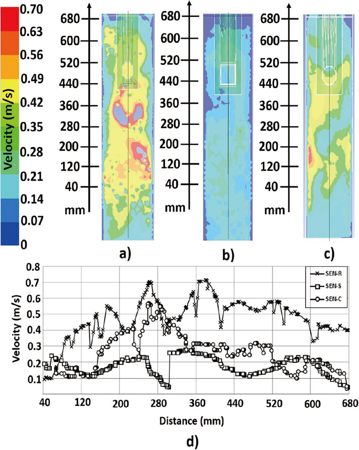
To get quantitative information about the behavior of each nozzle design, the velocity profile was plotted along a line located in the axis of the jet shown over the velocity contours computed through the mathematical model, Figs. 7(a), 7(b) and 7(c). The velocity scale at the plots was fixed at 0.7 m/s to observe a clear velocity distribution inside the mold. Obviously, the unfilled zones correspond a velocity higher than 0.7 m/s. The images presented here correspond to a computational time of 300 seconds. Figure 7(d) shows that the jet developed by the SEN-R has the highest velocity at the discharging ports (2.6 m/s) and the velocity fluctuations are visible along their path until impinging the narrow mold face with a velocity of 0.75 m/s. In contrast the SEN-S and the SEN-C have a velocity of 1.63 and 1.85 m/s at the discharging ports; respectively, their velocity profiles do not present considerable velocity fluctuations along their path until the narrow mold face are reached, where the impinging velocities were 0.12 and 0.4 m/s for SEN-S and SEN-C, respectively.

The high impinging velocities at the narrow mold face, yielded by SEN R, can affect the solidification front and promote breakouts problems, also the velocity at this zone governs the upper roll formation and, in consequence, the disturbances at the bath level.
To obtain a clear comparison among the three nozzles. The velocity profiles at the narrow mold mid face were plotted in Figs. 8(a)–8(c). It is evident that SEN-R has a larger area with high impinging velocity than the other two nozzles, indicating that the probability of washing the shell will be high.
The velocity profiles presented in Fig. 8(d) show that the SEN-S yields the lowest magnitudes the impinging velocities on the narrow mold face. Another important parameter is the velocity near the bath level (at 880 mm from the nozzle in Fig. 8(d). The SEN-R has values of 0.4 m/s, meanwhile the SEN-S and SEN-C present values less than 0.1 m/s. These large differences give the origin to surface instabilities, which will be discussed in the next section.
5.3. Free Surface Instabilities
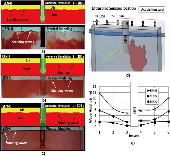
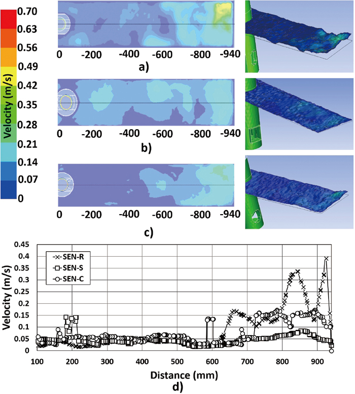
To observe the free surface behavior, velocity contours and their topology at the bath level zone were analyzed to compare qualitatively in Figs. 9(a)–9(c), and quantitatively, the performance of each SEN design in Fig. 9(d). The SEN-R, which develops a high velocity at near the narrow mold face (Fig. 8(d)), yields flows at the free surface with velocity peaks of 0.35 and 0.4 m/s, consequently, standing waves at the mold corners are formed, as can be observed in Fig. 9(a). The SEN-C yields flows at the free surface with velocities smaller than 0.2 m/s, and the standing waves are present but with less intensity and size in comparison with the SEN-R, Fig. 9(c). Meanwhile the SEN-S presents a very stable free surface without standing waves, as can be seen in the Fig. 9(b). The Fig. 9(d), shows that the zone of disturbance extends from the narrow mold wall to the middle of the mold.
To complement, qualitatively and quantitatively those results, video-images of the physical experiments were recorded and compared with the phase contours predicted by the VOF model, (Figs. 10(a)–10(c)). There is a good qualitative agreement between numerical and the physical approach. The meniscus level variations provided by the ultrasonic sensors (with locations indicated in Fig. 10(d) are plotted in Fig. 10(e). As seen the wave amplitudes provided by nozzle R are the largest followed by nozzles C and S. Indeed, as can be expected, high velocities at the narrow mold face, Fig. 9(d), yield high standing waves at the corners of the slab mold, Fig. 10(e). The SEN-R presents the highest free surface deformations along of all the free surface; meanwhile the SEN-S and SEN-C yield stable meniscus with very shallow depressions of standing waves, qualitatively indicating, that the flow at the free surface is less turbulent in comparison with the SEN-R.
5.3.1. Vortex Formation
Asymmetric flows parallel the wide faces of the mold induce secondary flows that pass with high velocities through the narrow gap between the SEN and the mold walls causing vortices that entrain slag. The slightest asymmetry can result in the formation of vortices, but this does not guarantee the entrainment of slag.11) To get drag slag by the melt, Gutierrez and Morales23) claim that the critical vortex necessary length is about 60 mm.
To compare the influence of each nozzle design on vortex formation, the number of vortices per minute and their size were measured from video recordings during the dye injection experiments. Figures 11(a)–11(c) shows some vortices recorded and measured for each SEN design. The SEN-R yields the maximum values of vortices per minute and average vortex length in comparison with the other two nozzle designs as can be seen in Figs. 11(d) and 11(e), respectively.
6. Closure
All simulations results are in good agreement with the physical experiments, confirming that increasing the discharging port transverse area decreases the turbulence level in the whole volume of the slab mold. Also, the SEN design definitely has a considerable influence in the dynamic of the flow, the SEN-R and SEN-C yield more turbulent flow than SEN-S.
The origin of the asymmetric flow is the turbulence level, but the consequences at the narrow mold faces and the free surface are the dissipation rate of turbulent kinetic energy. Figure 12 show that each nozzle dissipates kinetic energy at the discharging ports in diverse ways and intensity, and this behavior is extended to the whole flow in the mold.
All the results obtained from the physical experiments and numerical predictions were summarized in the Table 2. The maximum values of each presented variable were selected; and to obtain a clear conclusion about the best SEN design to use with the current operation conditions and mold size, the minimum values where remarked.
Table 2. Resume of results.
| VARIABLE | SEN-R | SEN-S | SEN-C | APPROACH |
|---|
| Jet misalignment* | 150 mm | 0 mm | 70 mm | Physical |
| Output velocity at discharging ports | 2.6 m/s | 1.63 m/s | 1.85 m/s | Numerical |
| Impinging velocity at narrow mold face | 0.7 m/s | 0.3 m/s | 0.6 m/s | Numerical |
| Depth of the jet impinging point** | 410 mm | 320 mm | 410 mm | Physical and Numerical |
| Horizontal velocity at free surface | 0.25 m/s | 0.05 m/s | 0.1 m/s | Physical |
| Surface wave height | 12 mm | 2 mm | 6 mm | Physical |
| Number of vortex per minute | 12 | 5 | 2 | Physical |
| Average vortex length | 44.5 mm | 16.4 mm | 13.7 mm | Physical |
| Dissipation rate of kinetic energy at discharging ports | 8.5 m2/s2 | 2 m2/s2 | 4.5 m2/s2 | Numerical |
* Is the difference between the depth of the jet impinging of the left and right side.
** Distance from the bath level to the jet impact point at the narrow mold face.
7. Conclusions
Fluid flow of liquid steel in a slab mold influenced by three different submerged entry nozzles with the same bore sizes but different ports SEN designs through numerical and physical modeling was studied. From the obtained results and their corresponding discussion, the following conclusions can be drawn:
(1) The results of the jet misalignment inside the mold indicate that two of the three nozzles develop asymmetrical flow inside the mold, but with different intensity, positioning the SEN-S and the SEN-R as the best and worst case studied, respectively (See Table 2).
(2) The global asymmetric flow inside the slab mold can promote a non-uniform heat transfer from the melt to the mold walls. In consequence, the solidification phenomena it can be affected and the cracks in the final product is very likely. Also, the large jet depth impact can affect the thickness of the first solidified shell, creating possible breakout problems.
(3) The velocity contours computed at the narrow mold face using the numerical approach reveals that the SEN-R and SEN-C, yields large areas affected by high velocity peaks (0.6 m/s using the SEN-C and greater than 0.7 m/s using the SEN-R), meanwhile the SEN-S yields impinging velocities of less than 0.3 m/s; thus, using this SEN design will result in less breakout problems.
(4) Another consequence of having asymmetric flow inside the mold, due to the instability of the jets, is the turbulence in the bath level zone (meniscus). Large velocities at meniscus promote slag entrainment by standing waves and vortex flows, which is the origin of inclusions problems in the final product. Physical and numerical results showed that the SEN-R develop the highest surface waves located at the corners of the mold. The SEN-R yield high horizontal velocities which travels from the narrow mold faces to the SEN body, where both flows (coming from the left and right side) converge and, potentiated by the surface waves, develop numerous vortex flows per minute (12 vortex/min) of great intensity and size (vortex average length of 44.5 mm). These vortex flows can drag slag into the liquid steel and explain the inclusions found in the final product at the plant.
(5) The contours of dissipation rate of kinetic energy at the discharging ports and the whole volume inside the slab mold indicate that the SEN-R and SEN-S develop the highest and lowest values, respectively. This last difference explains the behavior of the fluctuating jet observed at the velocity fields captured by the PIV technique. Therefore, the recommendation is to replace the SEN-R by the SEN-S to reduce the quality and operational problems reported in plant.
Acknowledgements
The authors give the thanks to CoNaCyT, PRODEP and the UA de C for their continuous support to the Mechanical Engineering Department.
References
- 1) R. Chaudhary, C. Ji, B. G. Thomas and S. P. Vanka: Metall. Mater. Trans. B, 42 (2011), 987.
- 2) J. Anagnostopoulos and G. Bergeles: Metall. Mater. Trans. B, 30 (1999), 1095.
- 3) Y. Miki and S. Takeuchi: ISIJ Int., 43 (2003), 1548.
- 4) A. Ramos-Banderas, R. Sanchez-Perez, R. D. Morales, J. Palafox-Ramos, L. Demedices-García and M. Díaz-Cruz: Metall. Mater. Trans. B, 35 (2004), 449.
- 5) L. Zhang and B. G. Thomas: ISIJ Int., 43 (2003), 271.
- 6) W. H. Emling, T. A. Waugaman, S. L. Feldbauer and A. W. Cramb: Steelmaking Conf. Proc., Vol. 77, ISS, Warrandale, PA, (1994), 371.
- 7) B. G. Thomas: The Making, Shaping and Treating of Steel, 11th ed., Casting Volume, ed. by A. W. Cramb, AISE Steel Foundation, Pittsburgh, PA, (2003), 24.
- 8) J. Herbertson, Q. L. He, P. J. Flint and R. B. Mahapatra: Steelmaking Conf. Proc., Vol. 74, ISS, Warrandale, PA, (1991), 171.
- 9) B. G. Thomas, Q. Yuan, S. Sivaramakrishnan, T. Shi, S. P. Vanka and M. B. Assar: ISIJ Int., 41 (2001), 1262.
- 10) I. Calderón-Ramos and R. D. Morales: Metall. Mater. Trans. B, 46 (2015), 1314.
- 11) L. C. Hibbeler and B. G. Thomas: Iron & Steel Technology Conf. and Exposition (AISTech) Proc., AIST, Warrandale, PA, (2010), 17.
- 12) S. Sivaramakrishnan: Master’s thesis, University of Illinois at Urban-Champaign, Urban, (2000).
- 13) E. Torres-Alonso, R. D. Morales, S. García-Hernández and J. Palafox-Ramos: Metall. Mater. Trans. B, 41 (2010), 583.
- 14) S. García-Hernández, R. D. Morales, J. de J. Barreto and K. Morales-Higa: ISIJ Int., 53 (2013), 1794.
- 15) U. Schumann: J. Comput. Phys., 8 (1975), 376.
- 16) K. Horiuti: J. Phys. Soc. Jpn., 54 (1985), 2855.
- 17) S. B. Pope: Turbulent Flows, Cambridge University Press, Cambridge, London, (2000), 771.
- 18) U. Schumann: Theor. Comput. Fluid Dyn., 2 (1991), 279.
- 19) W. W. Kim and S. Menon: AIAA Paper 97-0210, American Institute of Aeronautics and Astronautics (AIAA), New York, (1997), 325.
- 20) C. W. Hirt and B. D. Nichols: J. Comput. Phys., 39 (1981), 201.
- 21) P. Liovic, J. L. Liow and M. Rudman: ISIJ Int., 41 (2001), 225.
- 22) Fluent Inc.: Fluent Guides, Fluent Inc., Lebanon, NH, (2007).
- 23) Y. S. Gutierrez-Montiel and R. D. Morales: ISIJ Int., 53 (2013), 230.