Determination of Size Distribution of Nanoparticles Using Asymmetric Flow Field-flow Fractionation (AF4)

Abstract

To investigate the performance of the size measurement by asymmetric flow field-flow fractionation (AF4), the measurement results of gold nanoparticles were compared among AF4, transmission electron microscopy (TEM), and small-angle X-ray scattering (SAXS) in terms of the average size and full width at half maximum (FWHM) of the size distribution. Although the average size was almost the same for the three methods, the FWHM measured using AF4 was larger than those measured using TEM and SAXS. This is attributed to the diffusion of the gold nanoparticles inside the AF4 instruments. The broadening coefficient of AF4 analysis was determined as 2.08 by the average of FWHM ratio of AF4 to TEM measured using the several sphere-like gold nanoparticles. In addition, the effect of particle shape on the above broadening coefficient was investigated using the sphere-like and plate-like silver nanoparticles. The broadening coefficient for plate-like particles apparently became smaller than that for sphere-like particles, possibly because the Brownian motion of plate-like particles was suppressed.

Furthermore, the AF4 analysis with the FWHM correction method using the broadening coefficient was applied to niobium carbide (NbC) precipitates in steels. The average size measured by AF4 was mostly consistent with the results obtained in regions observed by TEM. Moreover, an increase in the number density of nanometer-sized NbC by heat treatment was successfully detected. The effect of particle shape on FWHM should be further investigated and improved; however, AF4 with the broadening coefficient can semi-quantitatively analyze the size distribution of nanoprecipitates in steels.

1. Introduction

Recently, nanoparticles, such as gold,^1,2) silver,³⁾ platinum,⁴⁾ carbon nanotubes, carbon black, and quantum dots,⁵⁾ have been used in various industries, including cosmetics, electronics, and food. Nanoparticles are defined as materials with a diameter of 1–100 nm. Steels contain various particles whose size ranges from nanometer to sub-micrometer for functionalizing various steel products.^6,7) The performance of particles in steels is dependent on their size and number density. In many cases, these particles have a wide size distribution; thus, determination of the average size and the size distribution of these particles has become considerably important. In particular, it is difficult to measure particles that have a wide size distribution (e.g., mixtures of several nanometers and several hundred nanometers particles) using conventional light scattering measurements and transmission electron microscopy (TEM). Moreover, the shape and chemical species of particles should be particularly considered while analyzing steels, because they exist in various shapes and types. It is well known that the influence of several particles co-existing in a same system is different for each measurement method, as follows. For dynamic light scattering (DLS),⁸⁾ the strength of scattered lights is strongly dependent on particle size. Thus, the strong lights scattered from larger particles apparently hide the weak lights scattered from smaller particles. However, there is a high risk of obtaining incorrect results in case of measurement for mixtures of small and large particles.⁹⁾ Furthermore, because the hydrodynamic diameter is estimated as that of spherical particles, it is much more difficult to accurately measure mixtures of various sizes and shapes. In case of TEM observations,¹⁰⁾ monodispersed particles can be easily observed; however, mixed particles with different sizes are often observed as particles with incorrect size through physical hiding, which results in small particles being missed. These methods have a common problem: the mixed particles with different sizes dispersed in a solution cannot be distinguished.

Hence, for accurately measuring the size distribution, separation techniques are necessary before measuring particles. Several size-based separation techniques, such as asymmetric flow field-flow fractionation (AF4), size-exclusion chromatography, hydrodynamic chromatography, gel electrophoresis, capillary electrophoresis, and ultracentrifugation, have been reported in previous studies.^{11,12,13,14,15)} Many studies have suggested that AF4 has some advantages for analyzing metallic nanoparticles.^16,17) AF4 has been employed for various samples, including certain matrices whose size ranges from nanometer to micrometer. If AF4 is combined with DLS and inductively coupled plasma-mass spectrometry (ICP-MS), the size distribution and elemental composition can be determined.^18,19,20) Thus, AF4 analysis is expected to accurately measure particles that have a nonuniform and wide size distribution (e.g., precipitates and inclusions in steels). However, the application of AF4 analysis to complex materials such as steels has not been performed yet.

In this study, prior to application to the evaluation of steels, the performance of size measurement by AF4 was investigated using gold nanoparticles (AuNPs). The average size and width of size distribution were verified by comparing the AF4 results with those of TEM and small-angle X-ray scattering (SAXS). Moreover, based on their results, a broadening coefficient for correcting the size distribution measured by AF4 was developed. Furthermore, the applicability of AF4 measurement with the broadening coefficient was investigated using niobium carbide (NbC) in steels.

2. Experimental

2.1. Nanoparticles and Reagents

All AuNPs and AgNPs were purchased from nanoComposix (San Diego, USA). All polystyrene size standard latex (PSL) particles STADEX were purchased from JSR life science (Tokyo, Japan). Tables 1 and 2 summarize the specifications of reference nanoparticles dispersed in water and those of the specimens. AuNP-2, AuNP-5, AuNP-7, and AuNP-10 were used for calibrating the size measurement for AF4 analysis. AuNP-5.5 was prepared for comparisons between AF4 and SAXS measurements; it was placed onto a carbon-supporting grid and observed in a bright-field image using TEM. Two types of AgNPs (sphere-like and plate-like, called AgNP-50s and AgNP-50p, respectively) were used for the size distribution measurement using AF4 and TEM. Furthermore, to measure AgNPs, AuNPs and PSL particles were used for the size calibration using AF4.

Table 1. List of nanoparticles for reference.

Sample	Average diameter (nm)	Concentration (mg/L)	Dispersant	Shape
AuNP-2	2.1 ± 0.3	52.5	Glutathione	Sphere-like
AuNP-5	5.0 ± 0.6	1080	Citrate	Sphere-like
AuNP-7	7.5 ± 0.8	1070	Citrate	Sphere-like
AuNP-10	9.8 ± 0.8	1080	Citrate	Sphere-like
PSL-29	29 ± 1	5000	–	Sphere
PSL-48	48 ± 1	10000	–	Sphere
PSL-70	70 ± 1	10000	–	Sphere
PSL-100	100 ± 3	10000	–	Sphere

Table 2. (a) Sample specifications and (b) an average diameter of each specimen measured by different analyses.

(a)

Sample	Concentration (mg/L)	Dispersant	Shape
AuNP-5.5	1090	Lipoic acid	Sphere-like
AgNP-50s	20	Tannic acid	Sphere-like
AgNP-50p	20	PVA	Plate-like
NbC precipitates in steel (NCA5-3)	–	SDS	Plate-like
	–	SDS	Plate-like
NbC precipitates in steel (NCA5-1)	–	SDS	Plate-like

(b)

Sample	Average diameter (nm)
	TEM	AF4 (raw data)	AF4 (corrected)	SAXS
AuNP-5.5	5.5 ± 0.5	5.6 ± 1.0	5.6 ± 0.5	5.0 ± 0.2
AgNP-50s	52.1 ± 7.1	54.1 ± 11.1	–	–
AgNP-50p	56.2 ± 14.6	59.6 ± 23.0	–	–
NbC precipitates in steel (NCA5-3)	2.4 ± 1.0 (FOV-1)	2.0 ± 0.4	2.0 ± 0.2	–
	2.1 ± 0.4 (FOV-2)			–
NbC precipitates in steel (NCA5-1)	–	2.1 ± 0.5	2.1 ± 0.2	–

All chemicals used for AF4 measurements were used as purchased without additional purification. Ultrapure water (>18 MΩ: Milli-Q water purification system type and Elix UV10, Millipore Corp., USA) was used for diluting samples and preparing AF4 carrier solutions. Sodium dodecyl sulfate (SDS, purity ≥ 99.0%) was obtained from FUJIFILM Wako Pure Chemical Corporation, Japan. Acetyl acetone (AA, special-grade, FUJIFILM Wako Pure Chemical Corporation), tetra methyl ammonium chloride (TMAC, purity ≥ 98.0%, Tokyo Chemical Industry Co., Ltd.), and methanol (special-grade, FUJIFILM Wako Pure Chemical Corporation) were used for extracting the precipitates from the steel sheets.

2.2. Sample Preparation via Selective Potentio-static Etching by the Electrolytic Dissolution Method

NbC-precipitated ferritic steel, whose main chemical composition is 0.1% Nb and 0.01% C (mass%), was prepared from electrolytic iron by vacuum induction melting. Brock specimens (30 × 33 × 45 mm³) for heat treatment were taken from an as-cast ingot. The heat treatment was conducted at 873 K for 1 h or 10 h after a solid solution treatment (1523 K, 24 h) and water quenching, which led to NbC precipitation. The holding time of the heat treatment was adjusted to change the size or number density of NbC. Additionally, the small specimens were cut into dimensions of 25 × 25 × 2 mm³ for the following analysis.

For obtaining specimens of precipitates formed in the steel sheets, selective potentio-static etching by electrolytic dissolution (SPEED)²¹⁾ was applied. A 10% (v/v) AA, 1% (w/v) TMAC, and 10 μg mL⁻¹ SDS-MeOH solution was used. The electrolytic extraction was conducted in two steps with a constant current of 500 mA. The first step was the pretreatment of the electrolytic extraction for cleaning the surface. This step was operated for 15 min to dissolve the pollutants on the surface and the oxide layer on the sample. The second step was conducted for the dissolution of the sample from the surface layer. To separate the surface pollutants and the oxide layer, which were dissolved in the electrolytic solution used in the first step from the sample, the second step was conducted for 120 min after transferring the sample to another electrolytic solution having the same components. After 120 min of the electrolytic treatment, ~1.0 g of the steel anode sample dissolved in the solution and nanometer-sized carbides were dispersed in the electrolytic solution.

2.3. Instruments

2.3.1. AF4-ICP-MS

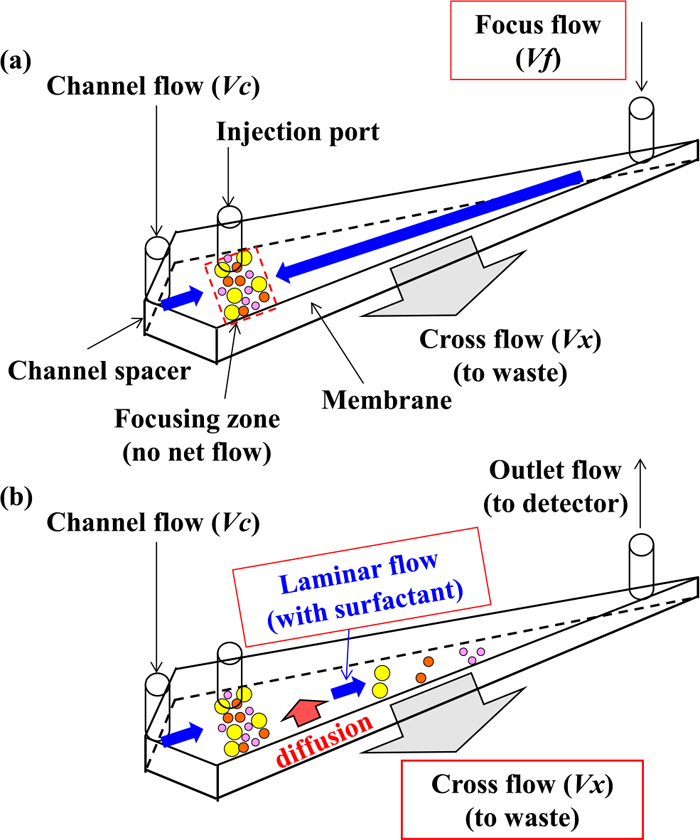
Figure 1 shows a schematic of Wyatt Eclipse AF4 system (Wyatt Technology Europe, Germany), which is combined with the ICP-MS system. This system is equipped with a high-performance liquid chromatography pump, an integrated degassing system, and an autosampler (Agilent Technologies 1260 Infinity series, Agilent Technologies, USA). After injecting nanoparticles into the AF4 separation channel, they were diffused and moved using a channel flow and separated in this system. During this time, 10 μg mL⁻¹ SDS solutions in ultrapure water were used as AF4 carrier solutions. Moreover, a regenerated cellulose (RC) ultrafiltration membrane (Microdyn-Nadir, Germany) with a molecular weight cut-off of 30 kDa (RC 30 kDa) was used as an accumulation wall for the AF4 separation channel. Then, the separation device with a 275-mm-long channel was employed, which was equipped with a 490-μm-thick asymmetric diamond-shaped channel spacer. The AF4 separation channel was connected to a variable-wavelength ultraviolet (UV)-visible detector (Agilent Technologies 1260 Infinity series) through a polyether ether ketone (PEEK) tube. The detection wavelength was set to 520 or 254 nm, and the online elemental information of the nanoparticles separated by AF4 was obtained using ICP-quadrupole MS (Agilent8800, Agilent Technologies, USA). This instrument was directly connected to the PEEK tube at the outlet from the UV detector of the AF4 system.

Fig. 1.

Schematic of the AF4 instrument. Flow profile observed during the (a) focusing step and (b) elution step. (Online version in color.)

The sample introduction system comprised a self-aspirating nebulizer (MicroMist nebulizer). Table 3 summarizes the operating conditions of ICP-MS. Prior to the AF4 measurement, the membrane was conditioned with an AF4 carrier solution of SDS for at least 30 min. Each AuNP and AgNP dispersed solution was diluted to 25 μg mL⁻¹ using ultrapure water. The precipitates dispersed in the SPEED solution were then applied without dilution. Then, these samples were injected in the AF4 separation channel using the autosampler, and then analyzed. Table 4 summarizes the AF4 separation conditions.

Table 3. Operating conditions of the inductively coupled plasma mass spectrometry (ICP-MS) when connecting to AF4.

Agilent8800 ICP-MS
RF power (W)	1550
Nebulizer flow (L/min)	1.05
Cooling gas (L/min)	15
Auxiliary gas (L/min)	0.90
Sampling depth (mm)	8
Element (m/z)	Au (197)
Duration time (s)	0.10
Spray chamber temperature (K)	275.15

Table 4. Separation condition in AF4.

		For AuNPs and NbC precipitates	For AgNPs
Channel parameters	Membrane nature	Regenerated Cellulose (RC)	Regenerated Cellulose (RC)
	Membrane cut-off	30 kDa	5 kDa
	Spacer	490 μm	350 μm
	Elution solvent	0.035 mmol L−1 SDS	1.73 mmol L−1 SDS
Fractionation time	Elution time	1 minute	1 minute
	Focusing time	1 minute	1 minute
	Focus + Injection time	2 minutes	2 minutes
	Focusing time	1 minute	3 minutes
	Elution time	45 minutes	35 minutes
Fractionation step, flow, and volume	Injection volume	20–100 μL (optimal)	100 μL
	Injection flow	0.2 mL min−1	0.2 mL min−1
	Channel flow (Vout)	1.0 mL min−1	1.0 mL min−1
	Cross flow (Vc)	2.0→0.1 mL min−1 (linear gradient)	3.0→0 mL min−1 (linear gradient)
	Focus flow	3.0 mL min−1	3.0 mL min−1
Detector	UV absorbance	520 nm	254 nm

2.3.2. TEM

For TEM observation, AuNPs dispersed in the solution were placed on the carbon-supporting grid and dried under reduced pressure. These samples were then observed using a field-emission transmission electron microscope (Tecnai F20, FEI Inc., USA) at an acceleration voltage of 80 kV. Bright-field images were obtained for the AuNPs, and processed using the Digital Micrograph software package (Gatan Inc., USA); the maximum diameter of each of the 500 particles was manually measured. Furthermore, the precipitates extracted in the above SPEED solution were prepared in the same manner as that for the TEM observation of AuNPs.

2.3.3. SAXS

SAXS measurements were performed at the beamline BL-10C,²²⁾ located at the Photon Factory (PF), the High Energy Accelerator Research Organization (KEK) in Tsukuba, Japan. The energy of an incident X-ray was set to 12.4 keV. A two-dimensional (2D) hybrid pixel array detector, PLATUS3 2M (DECTRIS Ltd., Baden, Switzerland), was set at 1 m from the sample. In the SAXS measurement, to measure the AuNPs dispersed in the solution, a custom-made sample cell was used for solution experiments. All SAXS measurements were performed as follows. The X-ray scattering data from AuNPs were obtained by measuring 10 frames with an exposure time of 10 s, and combined to yield a dataset with low noise. The obtained 2D data were converted to one-dimensional data [data obtained via circular ring average using Fit2d (developed by ESRF)]. Silver behenate was used for calibrating the camera distance. Furthermore, the scattering vector is defined as   

$$q=\frac{4\pi }{\lambda }sin\frac{\theta }{2}$$(1)

where λ is the wavelength (nm) and θ is the scattering angle. Note that the scattering intensities were corrected for background scattering.

2.4. Outline Principles of AF4 Measurements

In AF4 analysis, the separation sequence comprised the following four steps: sample injection, focusing, relaxation, and elution.²³⁾ First, samples were injected in the AF4 separation channel, and then collected in the focusing zone (Fig. 1(a)). Subsequently, they were diffused upward in the vertical direction, with the diffused distance dependent on the sample size. With a smaller size, the sample could be diffused far away, known as the relaxation step. Finally, the channel flow was changed in the elution step (Fig. 1(b)), and particles in the sample were separated by the difference in the flow rate in a laminar flow; consequently, smaller particles were detected with a faster retention time. In this case, according to the Stokes–Einstein equation, the diffusion coefficient had considerable influence on AF4 separation.²⁴⁾

3. Results and Discussion

3.1. TEM Observation of Nanoparticles

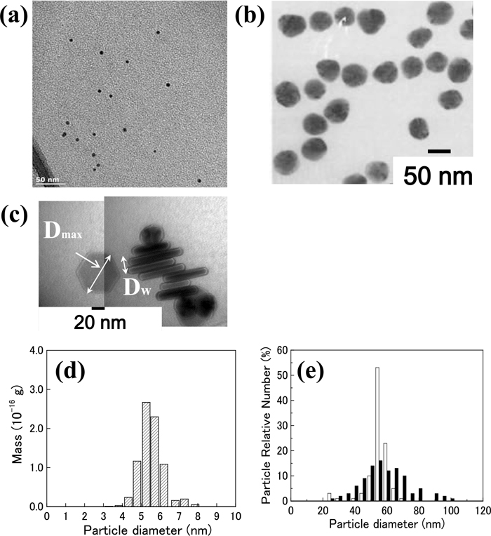
First, AuNP-5.5, AgNPs, and NbC precipitates were observed using TEM. AuNP-5.5 and AgNPs were dispersed not as aggregates but as single particles with a primary diameter. Figure 2 shows one of the TEM images and the size distribution of AuNP-5.5 and AgNPs; however, as shown in Fig. 3, certain NbC precipitates were aggregated in several fields of view (FOVs). The shape of AuNP-5.5 and AgNP-50s was almost spherical, but a part of the particles was not spherical; however, AgNP-50p and NbC precipitates had a plate-like shape. The diameter and thickness of AgNP-50p were approximately 56 and 14 nm, respectively. Furthermore, NbC precipitates had diameter and thickness of several nanometers. These nanoparticles were measured by AF4 and SAXS in subsequent experiments.

Fig. 2.

TEM bright-field image of (a) AuNP-5.5, (b) AgNP-50s, and (c) AgNP-50p on a carbon-supporting grid. The size distribution of (d) AuNP-5.5 and (e) two types of AgNPs by TEM. The white bar shows AgNP-50s and the black bar shows AgNP-50p. The diameter of AgNP-50p was measured as a maximum of diameter (Dmax). The thickness of AgNP-50s (Dw) was ignored here.

Fig. 3.

HAADF-STEM image of electrolytically extracted NbC from the steel sheet, NCA5-3, at two FOVs and size distributions at each FOV: (a) FOV No. 1 and (b) FOV No. 2.

3.2. Comparison of AF4 Results with TEM and SAXS Results in AuNP Analysis: Average Diameter and Width of Distribution

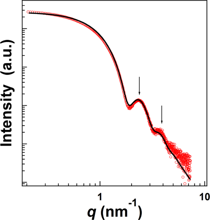
To confirm the performance of the size measurement method for AF4, AuNP-5.5 (primary diameter 5.5 ± 0.5 nm) was measured via AF4, TEM, and SAXS with synchrotron radiation. For AF4, the measurement was performed under optimized conditions, and the size distribution was estimated using the calibration curve obtained based on other AuNP sizes. The results were fitted via a Gaussian distribution, and the average size of AuNP-5.5 and the full width at half maxima (FWHM) of the size distribution were calculated. Furthermore, TEM observations were repeated twice to confirm the uncertainty of the size measurement using TEM. Moreover, for the SAXS measurement, the AuNP-5.5 dispersed solution was placed in a custom-made sample cell. Figure 4 shows the SAXS profile of the AuNP-5.5 dispersed solution. Two scattering peaks, indicated by arrows, were clearly observed. Generally, the scattering maxima from a form factor are clearly observed if the scatterers in a sample have a uniform size distribution. Thus, AuNPs were considered to have mostly uniform size. From the TEM observation, the shape of AuNP-5.5 was presumed to be spherical and the fitting was performed via a theoretical scattering curve. The form factor P(q) of the spherical particle was expressed in Eq. (2). The size distribution of P(q) was modeled using the Gaussian distribution. The solid lines in Fig. 4 show the calculated SAXS profiles. The calculated SAXS curves were in excellent agreement with the experimental curve.   

$$P\left(q\right)={\left(3C\frac{sin\left(qR\right)-qRcos\left(qR\right)}{{\left(qR\right)}^3}\right)}^2$$(2)

where C is a constant and R is the radius of the sphere.

Fig. 4.

SAXS profile of 5.5 ± 0.5 nm AuNPs. Solid line represents the model fits obtained using Eq. (2). (Online version in color.)

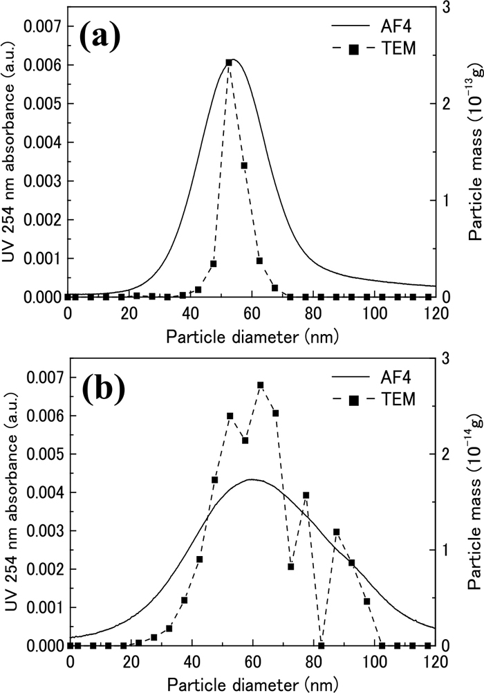
Figure 5(a) shows the results of AF4 analysis, SAXS fitting, and TEM observation. Table 2 summarizes each average size of AuNP-5.5 and the FWHM of the size distribution. As expected, the average size measured using AF4 was consistent with the TEM results, because AF4 measurement was conducted using the size calibration curve with TEM results. However, the two average diameters measured by AF4 and TEM were slightly larger than that of SAXS. This difference was caused by the presumption regarding the particle shape. For SAXS analysis, it was presumed that AuNPs had completely spherical shapes; however, the AuNPs were not completely spherical.

Fig. 5.

(a) Size distributions of AuNP-5.5 measured using AF4, TEM, and SAXS. The AF4 was operated under optimized conditions. TEM observations were repeated twice. (b) Comparison of size distributions of AuNP-5.5 among AF4, AF4 with broadening coefficient, and SAXS.

Furthermore, the FWHM of the size distribution measured by AF4 was not consistent with those measured by TEM and SAXS. The FWHM of the AF4 result was almost five times larger than that obtained using SAXS. Moreover, in the case of TEM, the FWHM of the AF4 result became approximately twice as large as that of TEM. These differences were attributed to the following two reasons. First, these methods for particle characterization adopted different principles for measurement. AF4 was used to measure particle mobility, TEM was used to measure electron diffraction, and SAXS was used to measure the difference in electron density in terms of crystallography. The AF4 result reflected the outer shape of the particles, the TEM result indicated the contrast of electron diffraction derived from elemental components and crystalline nature, and the SAXS result indicated the electron density difference between the particles and surrounding matrices. The difference in assumption regarding particle shape was reflected in these results.

Second, considerable attention should be paid to the measurement method in AF4 analysis, because the FWHM of size distribution measured by AF4 was the largest due to the diffusion of particles in the AF4 separation channel. Because the AF4 measurement was conducted under the condition that particles were flowing, it was unavoidable that any particle would diffuse in the AF4 separation channel. This phenomenon led to the broadening of the size distribution and a lack of size resolution; thus, the measurement method for particle size distribution using AF4 should be improved.

3.3. Correction Method for Size Distribution in AF4 Analysis

As discussed in 3.2, as FWHM largely depends on the principle, the measured values were attempted to be corrected for a realistic application. The correction method of the size distribution measurement for AF4 analysis was as follows. Each FWHM ratio of AF4 to TEM or SAXS for AuNP-5.5 was calculated from the results shown in Table 2; consequently, the FWHM ratio of AF4/SAXS and AF4/TEM was 4.64 and 1.94, respectively. The FWHM ratio of AF4/TEM should be adopted for the correction because the sizes estimated by TEM were used for the size calibration of AF4. The value was defined as a broadening coefficient of AF4 analysis. Additionally, same as mentioned above, the broadening coefficient for other nanoparticles was calculated, as shown in Table 5. Here, two types of AgNPs were measured by other AF4 operating conditions, because AgNPs had about 10-times larger diameter as compared to the above AuNPs. Prior to the AF4 measurement of AgNPs, the size calibration was conducted by several AuNPs and PSL particles, as shown in Fig. 6. The size distribution of two AgNPs measured by AF4 and TEM is shown in Fig. 7. It was revealed that the broadening phenomenon of particles in the AF4 separation channel can influence any AF4 chromatogram regardless of their particle size.

Table 5. The broadening coefficients in AF4 analysis.

Samples	Average size/nm (TEM)	Shape	Component of materials	Density/g·cm−3	Broadening coefficient	FWHM (AF4)	FWHM (TEM)
AuNP-2	2.1 ± 0.3	sphere-like	Gold	19.32	2.21	1.66	0.75
AuNP-5	5.0 ± 0.6	sphere-like	Gold	19.32	2.05	2.56	1.25
AuNP-5.5	5.5 ± 0.5	sphere-like	Gold	19.32	1.94	2.40	1.24
AuNP-7	7.5 ± 0.8	sphere-like	Gold	19.32	2.29	3.09	1.35
AuNP-10	9.8 ± 0.8	sphere-like	Gold	19.32	1.94	3.47	1.79
AgNP-50s	52.1 ± 7.1	sphere-like	Silver	10.49	3.01	26.09	8.66
AgNP-50p	56.2 ± 14.6	plate-like	Silver	10.49	1.64	54.05	32.90

Fig. 6.

Separation results of AuNPs and PSL mixtures by AF4. Bottom and right axes show the size calibration curve.

Fig. 7.

Size distributions of AgNPs measured using TEM and AF4. (a) AgNP-50s and (b) AgNP-50p.

The findings for the broadening coefficient are summarized as follows:

(i) The broadening coefficients calculated from the measurement results of the above AuNPs, largely depend on the shape and type of particles. The broadening coefficient determined for sphere-like particles was in a range of 1.94–2.29.

(ii) The effects of particle shape were considered for two types of AgNPs, because the direct comparison among different types of particles was not straightforward. The broadening coefficient for plate-like particles apparently became smaller than that for sphere-like particles. This was attributed to the fact that the flow in AF4 became more dominant than the Brownian diffusion of plate-like particles themselves; consequently, the Brownian motion of plate-like particles was suppressed for the horizontal direction.

Subsequently, the above broadening coefficient was used for calculating the standard deviation of AuNP-5.5. The average size measured by AF4, the total area of peaks detected by AF4, and the estimated standard deviation were utilized for correcting the size distribution measured by AF4. The Gaussian distribution was assumed from the TEM and SAXS results. Figure 5(b) shows the AF4 measurement results of AuNP-5.5 corrected by the broadening coefficient. It was revealed that the AF4 result calibrated by TEM became closer to SAXS result.

3.4. Application of Size Distribution Measurement Method by AF4 with Broadening Coefficient to NbC Precipitates in Steels

To investigate the applicability of the correction method of FWHM in AF4 analysis, NbC precipitates extracted from the steel samples were measured by AF4. Consequently, the correction method of FWHM was found to be more effective with a lesser measurement error for nanometer-sized precipitates in steels.

NbC precipitates were measured by AF4 under the operating conditions same as those for AuNPs. Figure 8 shows the size distribution of NbC precipitates measured by AF4. The heat treatment for steels was conducted to increase the size of NbC precipitates. Additionally, it was observed by TEM that these NbC precipitates were nonuniformly dispersed in the steel sheets. The size distribution of NbC precipitates was not coincident among several FOVs; however, AF4 showed average information about the size distribution and this result was almost close to that of TEM. Furthermore, this result indicated that not size but only the number density of fine NbC increased by about 1.5 times with the holding time of heat treatment, against our predictions. In this study, a quantitative analysis was not conducted due to the necessity of more improvement in the quantitativeness for AF4-ICP-MS. Because the peak areas of AF4-ICP-MS indicated the relative amounts of NbC, the difference in the number density of NbC was calculated through a comparison of peak areas between NCA5-1 and NCA5-3 steels: 1.0 and 1.5 respectively. In this manner, AF4-ICP-MS was found to be effective for semi-quantitatively measuring precipitates in steels.

Fig. 8.

Results of AF4-ICP-MS measurement for NbC in steels. The heat treatment was processed at 873 K to NCA5-1 (dotted line) for 1 h and to NCA5-3 (straight line) for 10 h.

In conclusion, the FWHM correction method in AF4 measurement was found to be useful for evaluating various nanoparticles. In the future, more detailed discussion would be conducted by considering the effect of particle shape on the FWHM of size distribution and improving the quantitative analysis method in AF4-ICP-MS.

4. Conclusions

The measurement method of the size distribution by AF4 with TEM was investigated using various nanoparticles. The findings in this study are summarized as follows.

(1) The average size measured by AF4 was almost same as those measured by TEM and SAXS. However, special attention should be paid to the presumption of particle shape, because the SAXS measurement was easily affected by the particle shape.

(2) For AF4 analysis, a peak-broadening phenomenon occurred because of the diffusion of particles in the AF4 separation channel.

(3) An FWHM correction method of size distribution in AF4 analysis was developed using a broadening coefficient, defined as the FWHM ratio of AF4/TEM.

(4) The broadening coefficient for sphere-like particles was determined as ca. 2.0; on the other hand, the broadening coefficient for plate-like particles (ca. 1.6) apparently became smaller than that for sphere-like particles due to the suppression of the Brownian motion.

When the broadening coefficient was applied, it was effective for the size evaluation of various nanoparticles. Therefore, the applicability of the FWHM correction method in the AF4 analysis was confirmed.

Acknowledgments

A part of this research was conducted under the institution “industrial use promotion of Photon Factory,” with the cooperation of the staff of Photon Factory. We would like to appreciate the staff’s cooperation.

References

• 1)   K. S.  Siddiqi and  A.  Husen: J. Trace Elem. Med. Biol., 40 (2017), 10.
• 2)   D.  Peng,  B.  Hu,  M.  Kang,  M.  Wang,  L.  He,  Z.  Zhang and  S.  Fang: Appl. Surf. Sci., 390 (2016), 422.
• 3)   H.  Chen,  F.  Gao,  R.  He and  D.  Cui: J. Colloid Interface Sci., 315 (2007), 158.
• 4)   Y.  Li and  F.  Zaera: J. Catal., 326 (2015), 116.
• 5)   T.  Jamieson,  R.  Bakhshi,  D.  Petrova,  R.  Pocock,  M.  Imani and  A. M.  Seifalian: Biomaterials, 28 (2007), 4717.
• 6)   N.  Kamikawa,  Y.  Abe,  G.  Miyamoto,  Y.  Funakawa and  T.  Furuhara: ISIJ Int., 54 (2014), 212.
• 7)   T.  Kataoka,  Y.  Arita,  F.  Takahashi,  H.  Fujimura,  Y.  Kurosaki,  M.  Sugiyama and  I.  Ohnuma: ISIJ Int., 56 (2016), 2062.
• 8)   M.  Filella,  J.  Zhang,  M. E.  Newman and  J.  Buffle: Colloids Surf. A, 120 (1997), 27.
• 9)   K.  Tiede,  A. B. A.  Boxall,  S. P.  Tear,  J.  Lewis,  H.  David and  M.  Hassellöv: Food Addit. Contam. Part A, 25 (2008), 795.
• 10)   M.  Hasselloev and  R.  Kaegi: Environmental and Human Health Impacts of Nanotechnology, ed. by J. R. Lead and E. Smith, Wiley Interscience, Bognor Regis, (2009), 211.
• 11)   G. T.  Wei,  F. K.  Liu and  C. R.  Chris Wang: Anal. Chem., 71 (1999), 2085.
• 12)   K. M.  Krueger,  A. M.  Al-Somali,  J. C.  Falkner and  V. L.  Colvin: Anal. Chem., 77 (2005), 3511.
• 13)   E. P.  Gray,  T. A.  Bruton,  C. P.  Higgins,  R. U.  Halden,  P.  Westerhoff and  J. F.  Ranville: J. Anal. At. Spectrom., 27 (2012), 1532.
• 14)   F. K.  Liu,  F. H.  Ko,  P. W.  Huang,  C. H.  Wu and  T. C.  Chu: J. Chromatogr. A, 1062 (2005), 139.
• 15)   X.  Xu,  K. K.  Caswell,  E.  Tucker,  S.  Kabisatpathy,  K. L.  Brodhacker and  W. A.  Scrivens: J. Chromatogr. A, 1167 (2007), 35.
• 16)   J. C.  Giddings: Science, 260 (1993), 1456.
• 17)   J. C.  Giddings,  F. J.  Yang and  M. N.  Myers: Science, 193 (1976), 1244.
• 18)   M.  Hassellöv,  B.  Lyvén,  C.  Haraldsson and  W.  Sirinawin: Anal. Chem., 71 (1999), 3497.
• 19)   B.  Schmidt,  K.  Loeschner,  N.  Hadrup,  A.  Mortensen,  J. J.  Sloth,  C. B.  Koch and  E. H.  Larsen: Anal. Chem., 83 (2011), 2461.
• 20)   H.  Hagendorfer,  R.  Kaegi,  J.  Traber,  S. F. L.  Mertens,  R.  Scherrers,  C.  Ludwig and  A.  Ulrich: Anal. Chim. Acta, 706 (2011), 367.
• 21)   K.  Takimoto,  I.  Taguchi and  R.  Matsumoto: J. Jpn. Inst. Met., 40 (1976), 834.
• 22)   N.  Igarashi,  Y.  Watanabe,  Y.  Shinohara,  Y.  Inoko,  G.  Matsuba,  H.  Okuda,  T.  Mori and  K.  Ito: J. Phys. Conf. Ser., 272 (2011), 012026.
• 23)   H.  Kato: AIST Bull. Metrol., 6 (2007), 185.
• 24)   M. E.  Schimpf,  K.  Caldwell and  J. C.  Giddings: Field-Flow Fractionation Handbook, Vol. 1, John Wiley & Sons, New York, (2000), 1.