1. Introduction
Fatigue is the principal cause of mechanical failures in structural materials. The fatigue crack can occur due to a variety of mechanisms. Defects such as inclusions and voids can be the origin of the fatigue crack initiations particularly in welding and casting materials. Since it is not practically possible or commercially feasible to always avoid the defects, it is necessary to consider the effect of the defects on the fatigue performance of these materials.
The inclusion acts as stress raisers, and the stress concentration depends on the shape and direction of the inclusion. In addition, fatigue failure due to multiple inclusions distributed in clusters has been reported.1,2) Therefore, it is clear that the behavior of defect-induced fatigue crack initiation is affected by the size, location and shape of the inclusions. To statistically investigate the effect of these inclusion features on the fatigue properties, a large number of experiments are required and it takes considerable time and costs. To overcome such problems on experiments, several physical models and empirical formulae have been proposed to predict the defect-induced fatigue properties. The Murakami’s model3) has been widely used to estimate the fatigue limit using hardness value and √area parameter (square root of the projected area of the inclusion on the plane normal to the tensile stress). Several numerical approaches for predicting fatigue life using the Murakami’s model have been proposed.4,5,6,7) Furthermore, more complex models that consider the arrangement of multiple inclusions are being examined.8,9,10) Salajegheh et al. have calculated fatigue indicator parameters using crystal plasticity simulations under different specimen sizes and inclusion sizes.8) They have also examined stress shielding or intensification effects by changing the position of two neighboring inclusions.9) Gillner et al. have investigated the effects of inclusion size and surface roughness by crystal plasticity simulations.10) With the rapid development of computer performance and software, three-dimensional (3D) numerical analysis is becoming more popular in recent years.11) In order to create a finite element model used for such 3D numerical analysis, detailed experimental data on the position and shape of inclusions in a 3D space is essential. Besides, the importance of modeling across multiple length scales is undoubtedly recognized in performance prediction of structural materials.12,13) A multi-scale modeling method for predicting fatigue life has been proposed in consideration of the hierarchical structure of materials.14,15,16,17,18) In order to reflect the effect of defects in these analyses, it is necessary to integrate information of defect distributions over multiple length scales.
The most commonly used method for obtaining the geometrical features of the inclusions is metallographic microscope observation (MMO) on a polished cross-section of small samples. The extreme value analysis is utilized to estimate the largest size inclusions in the effective size.19) The procedure is standardized in the ASTM E 2283.20) However, these two-dimensional (2D) observation methods cannot basically provide the 3D geometrical features of inclusions. In addition, the maximum inclusion size estimated by the extreme value analysis does not precisely coincide with the actual value. The estimated errors in the inclusion size can lead to significant error in fatigue life prediction. Recently, an automatic serial sectioning system with precision cutting and optical microscopy has been developed to achieve accurate 3D observation of the internal microstructure of materials.21) The system was successfully applied to investigate 3D shapes and positions of continuously distributed inclusion within bearing steel. This method provides the actual morphology of inclusions. However, the observation range is limited due to the time consumption and complexity of the procedure. On the other hand, ultrasonic testing (UT) allows us observation of a wider area. Since the UT provides non-destructive and online detection of defects, it is also suitable for industrial applications. However, it should be noted that UT method may miss small inclusions of a few micrometers.
As described above, each observation method has both advantages and limitations. In order to quantitatively evaluate the effect of inclusions on fatigue, it is required to (1) accurately measure the 3D shapes of inclusions, and (2) simultaneously evaluate small inclusions on the micrometer scale that form clusters and relatively large inclusions on the submillimeter. The purpose of this study is to combine defect distributions obtained by various observation methods such as MMO, serial sectioning, and UT across multiple scales. Based on the combined multiscale distribution, 3D shapes of inclusions on a wide length scale are characterized. As the target material, high-strength steel including a large amount of manganese sulfide (MnS) inclusions was prepared. The MnS inclusions are observed by mainly three methods: MMO, 3D internal structure observation with serial sectioning, and C-scan UT. The obtained images are analyzed to obtain the inclusion distributions of size, location, shape and direction. The obtained distributions are used in fatigue life prediction, and the effect of the inclusion distributions on the fatigue property will be discussed.
3. Results and Discussion
3.1. Inclusion Size Distribution Obtained by UT and Serial Sectioning
Figure 1 shows the polished cross-sections observed by MMO. Inclusions are clearly observed and their morphologies were rod-like shape elongated to R direction. According to EDX analysis, these inclusions were identified as MnS.

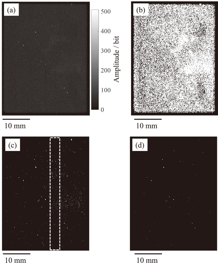
In the UT method, the amplitude data was acquired as a 10-bit grayscale image with the size of the scanned area. There are 1024 different levels of amplitude in the 10-bit grayscale image. The images were then binarized with several threshold levels of amplitude to obtain the probabilistic distribution of inclusion size. When the value at a scanned point exceeded the threshold, an inclusion was assumed to exist. Figure 2 shows examples of original amplitude data and the binarization results with the threshold levels of 50, 100 and 150. It clearly showed that the number and size of the inclusion changed with the threshold value. The inclusion size was converted to √area parameter24) for further analysis. Example of distribution of the √area parameters obtained by UT is shown in Fig. 3(a).

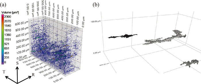
Using the automatic serial sectioning system, a total of 2650 cross-sectional images were acquired. Figure 4 shows examples of 3D reconstruction performed by VCAT and VGStudio. Inclusions with various sizes distributed over the analyzed block as shown in Fig. 4(a). Most inclusions were elongated to R direction. This finding was the same as that observed in MMO as shown in Fig. 1. The results of high-magnification observation of several large inclusions are shown in Fig. 4(b). These inclusions had flat shape elongated to R direction. The projected areas of inclusions on RT plane were calculated by VGStudio and converted to √area parameter. The distribution of √area parameters obtained by serial sectioning is shown in Fig. 3(b). The results showed that the serial sectioning method provided a statistical distribution of the inclusion size of a few micrometers that could not be captured by UT. On the other hand, it was difficult to obtain a statistical distribution of large inclusions exceeding 10 μm because the observation volume was much smaller than that in UT.
In order to cover multiple scales from micrometer to sub-millimeter, it is required to fit the obtained √area parameters to an appropriate probability density function (PDF). Several statistic distributions (gamma distribution, generalized extreme value distribution, lognormal distribution, exponential distribution, normal distribution and inverse Gaussian distribution) were applied to √area parameters obtained by serial sectioning. By comparing the log likelihood values obtained from each statistic distribution, generalized extreme value (GEV) distribution was considered to be the most appropriate PDF of the √area parameters. The GEV function is given by
|
f
GEV
(x;μ, σ, k)=
(
1
σ
)
exp[
-
{
1+k(
x-μ
σ
)
}
-
1
k
]
{
1+k(
x-μ
σ
)
}
-1-
1
k
,
| (1) |
where
μ is the location parameter,
σ is the scale parameter and
k is the shape parameter. The average values of
μ,
σ and
k obtained from 30 volume blocks were 1.66, 0.385 and 0.242
μm, respectively.
In order to combine the √area parameters obtained from UT to serial sectioning, it is necessary to identify a suitable threshold value of amplitude which provides the same √area distribution as those obtained from 3D observation. This can be made by using the root mean square logarithmic error (RMSLE) to find the threshold value that minimizes the error of PDF of √area data obtained from both methods:
|
RMLSE=
1
N
∑
(log
P
3D,func
-log
P
UT,exp
)
2
| (2) |
where
P3D,func is the extrapolated PDF obtained from 3D observation with serial sectioning and
PUT,exp is the PDF obtained by UT at a specific threshold value.
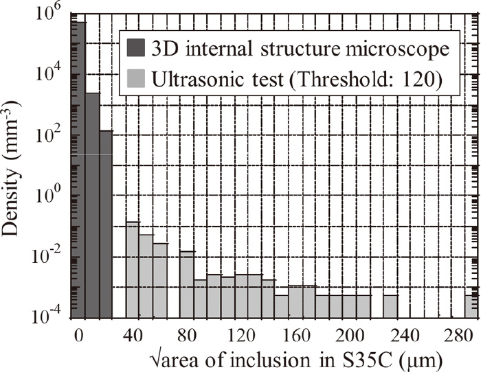
Figure 5 shows a plot of RMSLE as a function of threshold value. The RMSLE showed the lowest when the threshold was 120. With this threshold value, the √
area parameters and their number per unit volume obtained from both methods were plotted in
Fig. 6. As shown in the figure, the inclusion size distributions obtained by the two methods are smoothly connected on a wide length scale. Since an ordinary optical microscope observation on a single cross-section plane, the maximum √
area is not necessarily measured. In the observation by UT and serial sectioning, the maximum value of √
area can be acquired because the 3D shape of the inclusion is projected on a specific surface. Therefore, the inclusion size distribution obtained by UT and serial sectioning could be integrated by setting an appropriate threshold.

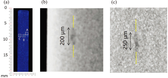
To examine the physical meaning of the threshold value in UT, a rod-shaped specimen was cutout from the area indicated by the dashed line in Fig. 2(b). As shown in Fig. 7(a), the UT results indicated that there were three large inclusions in the rod-shaped specimen (represented as A, B, and C in the figure). The √area parameters of inclusion A, B and C calculated by UT images with the threshold value of 120 were 112 μm, 137 μm, and 158 μm, respectively. The XCT images of the inclusion A and B are shown in Figs. 7(b) and 7(c). The inclusion C was not detected by XCT, probably due to its small thickness. The sizes of inclusion A and B were identified to be 200(R) μm × 50(T) μm × 20(S) μm and 250(R) μm × 50(T) μm × 20(S) μm, respectively. The √area parameters projected on the RT plane were 100 μm and 112 μm, respectively. To compare the results obtained from UT and XCT, the relationship between √area of inclusion and threshold value for UT is plotted in Fig. 8. The results of UT at a threshold value of 120 approximately correspond to those obtained by XCT. Therefore, it was suggested that the inclusion size could be appropriately evaluated by UT using the above threshold value. On the other hand, thin inclusions may not be detected by X-ray CT. In order to examine a more quantitative relationship between the inclusion size estimated by UT and the actual inclusion size, cross-sectional observations will be required in future works.
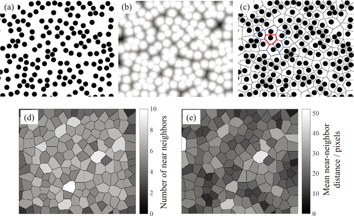
Based on the experimental data obtained in the previous section, the location of inclusions was evaluated by the coefficient of variation of the mean near-neighbor distance between inclusions (COVd),25,26) which is indicator of the inhomogeneity of spatial distribution. The calculation procedure of COVd is shown in Fig. 9. First, a binary image was created by placing spheres with position and size corresponding to the measured inclusions in a two-dimensional space (Fig. 9(a)). Then, the distance transformation was performed on the binary image. The distance transformation is one of the basic digital image processing methods, also called distance map or distance field. In this method, we focus on certain background pixel (white in Fig. 9(a)) and measure the distance from the focused pixel to the nearest object pixel (black in Fig. 9(a)). By performing this calculation for all background pixels, the distance value at each position is obtained. By assigning the distance as the brightness value of that position, the result can be plotted as in Fig. 9(b). The watershed segmentation was then performed on the distance transformed image. The Watershed algorithm is widely used in image segmentation and image edge detection. The brightness of the grayscale image (Fig. 9(b)) is regarded as a mountain peak, and the area created by the water flowing from the local highest points of the mountains (local maximum brightness points) is divided into one segment. As a result, the pixels with the low brightness value in the distance transformed image were defined as boundaries as shown in Fig. 9(c). The region enclosed by these boundaries was assigned as a finite body of the inclusions. When focusing on a certain inclusion finite body, the inclusion finite bodies surrounding the focused finite body were defined as the near-neighbor inclusions. Examples of near-neighbor inclusions are illustrated as a dotted line in Fig. 9(c). In the example shown in the figure, there are six near-neighbor inclusions. The number of near-neighbor inclusions for each inclusion is shown in Fig. 9(d). The distances between a certain finite body and the near-neighbor inclusions were calculated, and the mean value of the distances was referred to as “mean near-neighbor distance”. It is noted that the distance between finite bodies are different from the distance between the center points of the finite bodies. The above calculation was performed for all inclusions. The mean near-neighbor distance of each inclusion is shown in Fig. 9(e). By calculating the standard deviation and mean value for the mean near-neighbor distances of all inclusions, the coefficient of variation (ratio of the standard deviation to the mean value) was defined as the COVd. In the example of Fig. 9, the COVd is 0.324.
The calculation of COVd was performed on the optical images of the TR plane. The observation range per an image was 256 μm × 256 μm, and the resolution was 0.25 μm/pixel. The calculation was performed on a total of 34 images, and the total observation range was 2.22 mm2. Also, the COVd was calculated on the images obtained by UT with the threshold value of 120. The total observation range and resolution in UT were 1600 mm2 and 40 μm, respectively. The results of COVd in optical microscope and UT are shown in Table 3. In general, it has been shown that the COVd is close to 0, close to 0.36, and above 0.6 when inclusions are distributed uniformly, randomly, or in clusters, respectively.25,26) Both COVd values obtained from the optical microscope and UT were close to that of cluster-like distribution. Therefore, it was shown that inclusions of this material were arranged in clusters in 2D space. The above results also suggest that there are cluster-like distributions at two or more different scales.
Table 3. COV
d from optical microscope and ultrasonic test.
| Optical microscope | Ultrasonic test |
|---|
| COVd | 0.532 | 0.628 |
Additionally, the calculation of the COVd was performed in 3D space using the data obtained by 3D internal structure microscope with serial sectioning. The calculation procedure is the same as 2D images and consists of distance transformation, watershed imaging, and finite field tessellation. For comparison, the synthetic data in which inclusions were distributed uniformly, randomly and in clusters in 3D space were reproduced as shown Fig. 10. A uniform distribution (Fig. 10(a)) was created by arranging inclusions at regular intervals in the 3D space. A random distribution (Fig. 10(b)) was constructed by randomly sampling the inclusion positions (X, Y, Z) from the uniform distribution of each coordinate. The cluster-like distribution (Fig. 10(c)) was produced by determining the center position of the four clusters from a uniform distribution of (X, Y, Z) coordinates, and sampling 16 inclusion positions from a 3D Gaussian distribution with the center position of each cluster. In all cases, the number of inclusions was 64. The calculated COVd of uniform, random and cluster-like distributions were 0.035, 0.24 and 0.42, respectively. This revealed that the value of COVd in 3D space was lower than that in 2D space. For the experimental data of inclusions obtained by 3D internal structure microscope with serial sectioning, the COVd was calculated in the range of 855 μm × 641 μm × 90 μm. The calculated value of COVd was 0.40. Therefore, it was revealed that there were cluster-like distributions of inclusions also in 3D space.

The data of the 3D internal structure microscope was used to obtain the distributions of the inclusion shapes and directions. The calculation procedure is described below. First, 3D reconstruction was performed with VCAT on each inclusion observed by the 3D internal structure microscope. Then, the inclusion shape was smoothed using the free software Meshlab. The principal component score was calculated by performing principal component analysis (PCA) based on the nodal coordinates of the smoothed 3D data. The resulting principal component vectors correspond to the vectors of the major axis, medium axis and minor axis when the inclusion is fitted to an ellipsoid. Finally, an aspect ratio (minor axis/major axis) and an angle between the R direction and the major axis were derived as indices indicating the shape and direction.
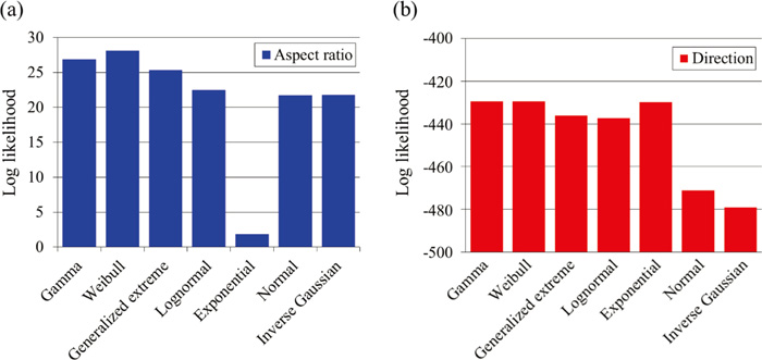
One hundred inclusions were prepared to conduct the above analysis and obtain the statistical distribution of the shape and direction. The 100 data points of shape and orientation were fitted to various PDFs: gamma distribution, Weibull distribution, generalized extreme distribution, lognormal distribution, exponential distribution, normal distribution and inverse Gaussian distribution. The log likelihood of each PDF is shown in Fig. 11. The PDF with the highest log likelihood was a Weibull distribution for the aspect ratio and a gamma distribution for the direction. The Weibull distribution is given by
|
f
weibull
(x;a,b)=
b
a
(
x
a
)
b-1
exp
(
-
x
a
)
b
,
| (3) |
where
a is the shape parameter (0.41) and
b is the scale parameter (1.95). The gamma distribution is given by
|
f
gamma
(x;α,β)=
1
β
α
Γ(α)
x
α-1
exp(
-
x
β
)
,
| (4) |
where
α is the shape parameter (0.907) and
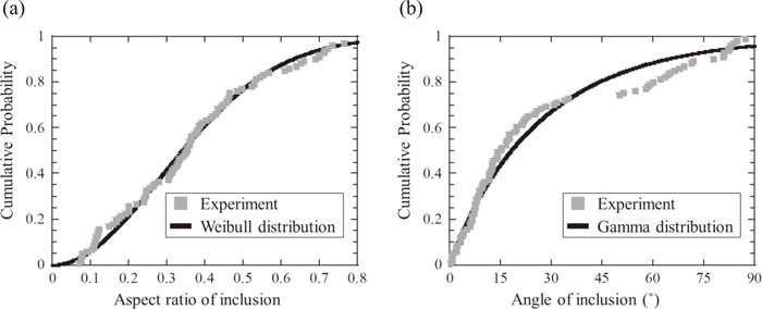
β is the scale parameter (29.9). The cumulative probability of the experimental values and the PDFs are shown in
Fig. 12. It can be seen from
Fig. 12(a) that inclusions with an aspect ratio of 2:1 or less occupy approximately 80% of the total. This is because the inclusions were elongated in the rolling direction. Similarly, the inclusions within an angle of 45° occupied approximately 70% in
Fig. 12(b). This result suggests that most inclusions are oriented in the rolling direction. From the above results, it was found that the distribution of the shape and direction of inclusions can be obtained by 3D internal structure microscope with serial sectioning. In future studies, analyzing local curvature and homology parameters may be useful for fatigue prediction. The local curvature is related to stress concentration and resultant fatigue crack formation. The homology parameters such as Betch number and Euler characteristic are related to connectivity of inclusions.
3.5. Application of Multiscale Size Distribution to Fatigue Life Prediction
As discussed in Section 3.2, observation with the 3D internal structure microscope revealed that the small inclusions formed complex cluster structures in the high strength steel. A part of relatively large inclusions detected by UT are considered to correspond with these inclusion clusters. As pointed out by Mughrabi,27,28) the arrangement of inclusions in the cluster plays a significant role on fatigue crack initiation. For example, Salajegheh et al. performed finite element analysis and showed that the effect of inclusion clusters on fatigue crack initiation decreases exponentially with increasing the inclusion spacing.9) The COVd derived in the present study would be useful for expressing the degree of clustering and assessing its effect on fatigue. On the other hand, in order to predict the fatigue life by considering the effect of inclusions, several probabilistic models that take into account the distributions of inclusion size and shape have been proposed.5,6,7) In this section, the obtained distributions of inclusion size, aspect ratio and direction were applied to the fatigue life prediction model developed by the authors7) without considering the effect of clusters for simplicity. In this model, the size, shape and orientation of inclusions are randomly sampled from the probability distributions obtained in the present study. Assuming a specimen having a gauge part of 2 mm × 2 mm × 10 mm, the inclusions were placed in the 3D space. In the simulation, it is assumed that cracks initiate from the grains adjacent to the inclusions, and the stress concentration depends on the shape and direction of the inclusions. The crack initiation life was predicted by the extended Tanaka-Mura model:29)
|
N
i
=
8G
W
c
π(1-ν)d
(Δτ-2
τ
c
)
2
,
| (5) |
|
k
t
=7.2937×
10
-7
θ
2
⋅A
R
2
-1.7204×
10
-5
θ
2
⋅AR+3.4779
×
10
-4
θ⋅A
R
2
-0.0024θ⋅AR+1.7857×
10
-5
θ
2
-0.0184A
R
2
+0.0017θ+0.1661AR+1.2479,
| (7) |
where
Ni is crack initiation life,
G is the shear modulus (76.9 GPa),
Wc is the fracture energy per unit area (2 kJ/m
2),
ν is the Poisson ratio,
d is the length of the slip band (50
μm), Δ
τ is the resolved shear stress range and
τc is the critical resolved shear stress for dislocation motion, Δ
σ is applied stress amplitude,
M is Taylor factor,
kt is stress concentration factor due to inclusions calculated by finite element method,
θ is the angle of inclusion against the loading direction and
AR is the aspect ratio of inclusion. For the all possible crack initiation sites, the crack propagation life was calculated by the Paris law:
|
N
p
=
1
C
(
QΔσ
π
)
m
∫
a
ini
a
f
da
(
Y'
a
)
m
,
| (8) |
where
Np is crack propagation life,
a is crack length,
C and
m are materials constants (C = 1.5 × 10
−11 m/cycle, m = 2.75),
aini is the initial crack length (sum of inclusion size and grain size),
af is the fracture crack length derived from the fracture toughness,
Q is 0.61 for surface defects and 0.47 for interior defects. The shape factor (
Y’) was defined by the following equations for the surface crack and the interior crack, respectively:
|
Y
'
surface
=
W
πa
×
2tan
πa
2W
cos
πa
2W
[
0.752+2.02(
a
W
)
+0.37
(
1-sin
πa
2W
)
3
],
| (9) |
|
Y
'
interior
=
sec(
πa
2W
)
[
1-0.025
(
a
W
)
2
+0.06
(
a
W
)
4
],
| (10) |
where
W is the specimen width. By comparing the total fatigue life (
Ni +
Np) for all crack formation sites, the minimum value is adopted as the prediction result. More detailed calculation procedures are described in the literature.
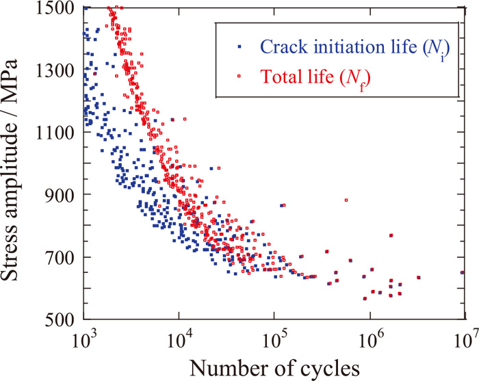
7) The stress ratio was set to
R = −1, and the stress amplitude was randomly sampled between 500 MPa and 1500 MPa. The calculation was repeated 1000 times. The calculation results are shown in
Fig. 13. It was found that the crack growth life occupies most of the total life under the high-stress amplitude (low cycle region) while the crack initiation becomes dominant under low-stress amplitude (high cycle region). Focusing on the results of the total fatigue life, the scattering became larger in the high cycle region. This trend is consistent with experimental behavior reported in numerous works of literature. Thus, it can be expected that the fatigue properties can be evaluated by using the inclusions distributions obtained by the multiscale analysis. In future work, the experimental data on the crack initiation life and total fatigue life will be required to validate the fatigue prediction model.