Modelling of Hydrogen Diffusion in a Weld Cold Cracking Test: Part 2, Numerical Calculations

Abstract

The purpose of this work is to compare the numerical calculation results of the hydrogen diffusion with the experimental results. We firstly conducted a y groove weld cracking test using 980 MPa grade steel and 780 MPa grade welding consumable to observe HAZ cracking. Next, we showed the present diffusion equation and the procedure to determine the physical properties for the calculations such as stress-strain curve, and using the apparent diffusion coefficient and the boundary condition obtained in the companion paper, we conducted the numerical calculations for the two cases, that is, the under-match case (980 MPa grade steel and 780 MPa grade welding consumable) and the even-match case (780 MPa grade steel and 780 MPa grade welding consumable). The calculation results of the under-match case show that hydrogen tends to accumulate in the stress concentration area of both the HAZ and the weld metal, which indicates crack may occur in both the HAZ and the weld metal. The results of the even-match case show not only the hydrogen accumulation around the stress concentration area but also high hydrogen concentration in the weld metal, which indicates crack may occur in the weld metal. Calculation results for both of the cases fairly agree with the experiments.

1. Introduction

The purpose of this paper is to conduct the numerical calculations of hydrogen diffusion in a y groove weld cracking test¹⁾ using the apparent diffusion coefficient (D_app) and the boundary condition obtained in the companion paper. The calculation results are compared with the experimental results to verify the present hydrogen diffusion model. At first, we conduct the y groove weld cracking test using the 980 MPa grade steel and 780 MPa grade welding consumable. This type of joint is called under-match joint. We select this type of joint to obtain HAZ cracking. Secondly, we conduct the numerical calculations of hydrogen diffusion and compare the calculation results with the experiments. Matsuda et al.²⁾ reported that cracking generally occurs in the weld metal when the strengths of the steel and the weld metal is 780 MPa or over. So we select the two cases for the calculations. The first case is of the present experiment, that is, under-match joint (hereafter, under-match case). As shown later, cracks firstly occur in the HAZ even though both of the strengths are 780 MPa grade or over. The second case is of even-match joint, that is, 780 MPa grade steel and 780 MPa grade welding consumable (hereafter, even-match case). Okamura et al.³⁾ developed a new type 780 MPa grade steel with high resistance to cold cracking and showed the y groove weld cracking test results with 780 MPa grade welding consumable. Their paper reported the crack occurred in the weld metal. The present numerical calculations are conducted using the D_app values calculated from the Vickers hardness (Hv) distributions of these two cases. We compare the calculation results with the experiments, and show that the present model agrees with the experimental results.

2. Weld Cold Cracking Test

2.1. Experimental Procedure

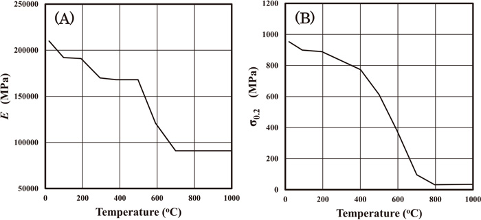
As a weld cold cracking test, we have chosen a y groove weld cracking test.¹⁾ The y groove weld cracking test is to examine cold cracking susceptibility of steel and is frequently used, especially in Japan. So we consider this test is adequate to compare the calculations with the experiments. Steel 5 in Table 1 is a 980 MPa grade steel and is for the y groove weld cracking test. Steel 5 is a laboratory melted steel. The chemical compositions were chosen considering the previous steel reported in the literature.⁴⁾ Steel 5 was rolled down to 35 mm thickness, and heated up to 1050°C for 3.6×10³ s and quenched into water, followed by tempering at 600°C for 1.2×10³ s. After that, the thickness of steel 5 was reduced to 30 mm by machining. To confirm that steel 5 is a 980 MPa grade steel, we preliminarily conducted the tensile test. The tensile test specimen was a cylindrical one machined at 1/4 thickness position of steel 5 with 6 mm diameter and 24 mm gauge length. Figure 1 shows the result of the tensile test, and the 0.2% proof and tensile strengths were 953 MPa and 1044 MPa, respectively. For the cracking test, we used the under-match welding electrode, that is, E11016-G welding electrode⁵⁾ (a 780 MPa grade electrode) for the crack to occur in the HAZ. We selected the two preheat temperatures, that is, 20°C (no preheating) and 125°C. The condition of no preheating was for crack observations, and the condition of 125°C preheating was to avoid crack and to measure the hardness distribution. According to the conventional hardness prediction method,⁶⁾ the hardenability of steel 5 is high. So we consider that the preheating has little influence on hardness distribution. The cracking tests were conducted in a room in which the ambient temperature and the relative humidity were kept 20°C and 60%, respectively. Five macro specimens from each test piece were machined, polished and etched with nital etchant to observe the cold cracks. The detail cracking test procedure is in JIS Z 3158.¹⁾ After confirming no crack in the case of 125°C preheating, we measured the hardness distribution of the macro specimen.

Table 1. Chemical compositions of steels used in this study (mass%).

Steel	C	Si	Mn	P	S	Ni	Cr	Mo	Nb	V	B
5	0.12	0.12	0.93	0.001	0.002	2.0	0.60	0.60	0.016	0.050	0.0010

Fig. 1.

Stress-strain curve of steel 5 and the comparison with Eq. (5).

2.2. Results

Figure 2 shows an example of the macro specimens machined from the y groove weld cracking test piece with no preheating. We can recognize that the cold crack firstly occurred at the stress concentration area of the HAZ and then propagated in the HAZ near the fusion line. After that, the crack went into the weld metal. The other four macro specimens exhibited the same initiation and propagation. As already mentioned, when the strengths of a steel and a weld metal are 780 MPa or over, cold cracks generally occur at the stress concentration area of the weld metal and propagate in the weld metal.²⁾ However, in the present work, since the tensile strength of the weld metal is lower than that of the steel, crack firstly occurred in the HAZ. Figure 3 shows the Vickers hardness (Hv) distribution of the macro specimen machined from the cold cracking test piece with 125°C preheating. We can see that H_V of the HAZ is the highest of the three and that H_V of the weld metal is the lowest. So Fig. 3 indicates that the welded joint of the present experiment is under-match joint. From Fig. 3, we consider the values of H_V for the base metal (BM), the HAZ and the weld metal (WM) are approximately 360, 400 and 340, respectively. These values will be used to calculate D_app for the numerical analysis later.

Fig. 2.

Macro specimen of the y groove weld cracking test with no preheating. Crack initiated at the stress concentration area of the HAZ, propagated in the HAZ and went into the weld metal.

Fig. 3.

Hardness distribution of the macro specimen of the y groove weld cracking test with 125°C preheating.

3. Diffusion Equation and Physical Properties of the Present Model

3.1. Governing Equation of Hydrogen Diffusion

Hydrogen diffusion is caused by the gradients of the hydrogen content, the stress, the temperature and the hydrogen diffusion coefficient. In the case of welded joints, these factors of hydrogen diffusion have to be taken into account. We firstly describe hydrogen flux, $\overrightarrow{j}$ (mol·mm⁻²s⁻¹) as follows.   

$$\overrightarrow{j}=-{\alpha }_1{D}_{app}\nabla C+{\alpha }_2\frac{D_{app}C\cdot V_H}{RT}\nabla {\sigma }_p+\overrightarrow{F}$$(1)

Here, R is gas constant (8.31×10³mJ· mol⁻¹K⁻¹), V_H is a partial molar volume of hydrogen (2.0×10³mm³mol⁻¹),⁷⁾ and σ_p (= (σ_x + σ_y + σ_z)/3) is hydrostatic stress (MPa). α₁ and α₂ are the phenomenological parameters proposed by previous literatures, named α multiplication method.^8,9,10) $\overrightarrow{F}$ denotes a term that will be discussed later.⁸⁾

The first term in the right side of Eq. (1) comes from Fick’s law that assumes the hydrogen flux proportional to the concentration gradient. There are some indications that Fick’s law should be replaced when there exist effects of trapping, non-uniform solubility and so on. Leblond and Dubois¹¹⁾ reported a diffusion equation more versatile than Fick’s law. McNabb and Foster¹²⁾ reported a diffusion equation with a trapping term. In this work, we have introduced the phenomenological parameter, α₁, to fit the calculations more closely to the experiments. The second term comes from the hard sphere model of hydrogen atom whose volume is V_H. The potential energy is described as −σ_pV_H, and the force acting on the hydrogen atom is hence V_H∇σ_p under the assumption of the constant volume. The phenomenological parameter, α₂, also has been introduced to fit the calculations more closely to the experiments. In addition, it may be considered that these two parameters, α₁ and α₂, represent the interaction between the ∇C and ∇σ_p driven diffusions.

The mass conservation law is as follows.   

$$\frac{\partial C}{\partial t}=-\nabla \overrightarrow{j}$$(2)

By substituting Eq. (1) into Eq. (2), we obtain the following diffusion equation.   

$$\begin{array}{l}{\displaystyle \frac{\partial C}{\partial t}}={\alpha }_1\left(D_{app}{\nabla }^{2}C+\nabla D_{app}\cdot \nabla C\right)\\ -{\alpha }_2{\displaystyle \frac{V_H}{R}}\left({\displaystyle \frac{C}{T}}\nabla D_{app}\cdot \nabla {\sigma }_p+{\displaystyle \frac{D_{app}}{T}}\nabla C\cdot \nabla {\sigma }_p-{\displaystyle \frac{D_{app}C}{T^2}}\nabla T\cdot \nabla {\sigma }_p\right)\\ -{\alpha }_2{\displaystyle \frac{V_H{D}_{app}C}{RT}}{\nabla }^2{\sigma }_p-\nabla \overrightarrow{F}\end{array}$$(3)

In the case of conservative (elastic) system, ∇²σ_p is zero. In this case the value of α₂ makes no difference to the ∇²σ_p term (the third term) in Eq. (3). Actually, Leeuwen¹³⁾ dropped the ∇²σ_p term from the diffusion equation. However, when plastic strain is introduced (non-conservative system), numerical calculations show that ∇²σ_p is not zero. This may indicate that the stress field is different from what the elastic model expects. This is the additional reason why the phenomenological parameter, α₂, has been introduced because the potential energy of hydrogen atom, −σ_pV_H, comes from the elastic model. Yokobori et al.⁸⁾ investigated the effect of the ∇²σ_p term on the hydrogen diffusion, and showed that the ∇²σ_p term operates as a source or a sink of hydrogen. But there is neither source nor sink of hydrogen in a welded joint, and hence we have introduced the $\nabla \overrightarrow{F}$ term to compensate this discrepancy. From their conclusion, we have introduced another phenomenological parameter, α₃, for the third and fourth terms in Eq. (3), and hence Eq. (3) has been rewritten as follows.   

$$\begin{array}{l}{\displaystyle \frac{\partial C}{\partial t}}={\alpha }_1\left(D_{app}{\nabla }^{2}C+\nabla D_{app}\cdot \nabla C\right)\\ -{\alpha }_2{\displaystyle \frac{V_H}{R}}\left({\displaystyle \frac{C}{T}}\nabla D_{app}\cdot \nabla {\sigma }_p+{\displaystyle \frac{D_{app}}{T}}\nabla C\cdot \nabla {\sigma }_p-{\displaystyle \frac{D_{app}C}{T^2}}\nabla T\cdot \nabla {\sigma }_p\right)\\ -{\alpha }_3{\displaystyle \frac{V_H{D}_{app}C}{RT}}{\nabla }^2{\sigma }_p\end{array}$$(4)

Equation (4) is the diffusion equation for the y groove weld cracking test used in the present work. In this work, we have quoted α₁, α₂ and α₃ values from the previous works.^{8,9,10,14,15,16)} They are set to be 1, 30 and 0.5, respectively. The boundary condition for the surface of the cracking test specimen and the empirical equation to calculate D_app are given in the companion paper. It is worth mentioning that Eq. (4) is identical to the diffusion equation of the hydrogen evolution test in the companion paper when D_app and temperature are constant, and there is no stress.

3.2. Physical Properties

The present model of hydrogen diffusion consists of three parts. The first part is for heat conduction analysis, the second part is for thermal elastic plastic analysis and the third part is for hydrogen diffusion analysis. In the first part, we used the conductivity of 0.054 (J·K⁻¹·mm⁻¹·s⁻¹) and the thermal diffusion coefficient of 12.0 (mm²/s).¹⁷⁾ These two physical properties of heat conduction are common between the under-match and the even-match cases. For the thermal elastic plastic analysis, stress-strain curves of the base metal, the HAZ and the weld metal are necessary. Here, we would like to describe the procedure to determine the stress-strain curves for the under-match case (the present experiment). The procedure can be easily applied to the even-match case.

At room temperature, the stress-strain curve of the base metal (steel 5 in Table 1) is given in Fig. 1. To describe the stress-strain curve, we consider the following equation.   

$$\sigma =\{\begin{array}{l}E\epsilon \hfill \\ 0.01E\left(\epsilon -{\sigma }_{0.2}/E\right)+{\sigma }_{0.2}\hfill \end{array}\hspace{1em}\begin{array}{c}\left(\epsilon \le {\sigma }_{0.2}/E\right)\\ \left(\epsilon >{\sigma }_{0.2}/E\right)\end{array}$$(5)

Here, σ_0.2 is 0.2% proof stress (MPa), and E is Young modulus (MPa). Equation (5) describes the nominal stress-strain curve. Why we have selected the nominal stress-strain curve will be shown later. Equation (5) assumes that the work hardening coefficient is E/100. Figure 1 shows the experimental stress-strain curve of steel 5 and Eq. (5) with E of 2.1×10⁵ MPa and σ_0.2 of 953 MPa. These two curves are in good agreement on the left of the ultimate stress. We can recognize that there exists the disagreement between the experiment and Eq. (5) on the right of the ultimate stress. This is because of the necking phenomenon that we do not have to take into account in the case of the cracking test, and hence we consider that this disagreement is not crucial. So we use the stress-strain curve of Eq. (5) for the base metal, steel 5. Temperature dependences of Young modulus and the 0.2% proof stress are shown in Fig. 4, which are from Mikami et al.¹⁸⁾ Figure 4(B) was obtained by slightly modifying their data considering that the 0.2% proof stress of steel 5 is 953 MPa. Using Eq. (5) and Fig. 4, we can determine the stress-strain curve of the base metal at each temperature. For the HAZ and the weld metal, we assume that Young modulus of these two regions is the same as that of the base metal, Fig. 4(A), but we modified the profiles of the 0.2% proof stress for these two regions using the Vickers hardness values. We assume that the value of the 0.2% proof stress is proportional to the hardness value. For example, the 0.2% proof stress of the HAZ at room temperature can be calculated as 953‧400/360=1059 MPa. The temperature dependences of the 0.2% proof stresses of the HAZ and the weld metal can be determined from Fig. 4(B) in this way. Finally, we determined the stress-strain curves of the three regions at each temperature using Eq. (5). Poisson ratio and thermal expansion coefficient were selected as 0.3 and 0.000012 (1/K), respectively.

Fig. 4.

Temperature dependences of Young modulus E (A) and 0.2% proof stress σ_0.2 (B).

In the next section, we will also conduct the numerical calculations for the experiments in the literature as the even-match case. The hardness distribution of the even-match case is different from that of the under-match case, but the procedure to determine the stress-strain curves will be applied to the even-match case using its hardness distribution. As to Young modulus, Poisson ratio and thermal expansion coefficient, we use the same values, that is, Fig. 4(A), 0.3 and 0.000012 (1/K), respectively. Once the physical properties of the heat conduction and the thermal elastic plastic analyses are determined, D_app (the physical properties of the hydrogen diffusion analysis) can be determined. So we can conduct the numerical calculations of the present hydrogen diffusion model.

4. Numerical Calculations and Discussion

4.1. Outline of the Present Hydrogen Diffusion Model

The present model consists of the heat conduction analysis, the thermal elastic plastic analysis and the hydrogen diffusion analysis. The calculation of the heat conduction is carried out with FDM and the results are input to the thermal elastic plastic analysis. In the thermal elastic plastic analysis, the calculations are conducted with FEM. The calculation results of these analyses such as temperature, stress and plastic strain distributions are input to the hydrogen diffusion analysis. In the hydrogen diffusion analysis, the calculations are carried out with FDM considering the stress driven diffusion. The temperature and plastic strain distributions are used to determine the values of D_app. The effect of stress distribution is considered by the stress dependent term in the diffusion equation.

Figure 5 shows the outline of the present model. At the beginning, the information of steel, welding consumable and welding condition is input to the model. As mentioned in the companion paper, the hardness is selected as a representative of the microstructure. In the present model, the hardness distribution of an interested joint is treated as input data. The hardness distribution may be experimentally obtained or predicted using the conventional prediction methods.^6,19) After information is input, heat conduction analysis is carried out by FDM. Since the calculated temperature values by FDM are obtained as grid values, they are interpolated to nodal points of FEM for the thermal elastic plastic analysis. In the thermal elastic plastic analysis, the values of stress and plastic strain are obtained as nodal values of FEM. These values are interpolated to grid points of FDM for hydrogen diffusion analysis. The detail of the interpolation method is described previously.⁸⁾ In the diffusion analysis, not only the calculation results of temperature and plastic strain but also the hardness values are used to determine D_app. After the completion of the diffusion analysis of this step, the next step will start.

Fig. 5.

Outline of the present hydrogen diffusion model.

4.2. Model for the Y Groove Weld Cracking Test

Figure 6 shows the dimensions of the y groove weld cracking test specimen. The thickness is 30 mm, which is the same of the present experiment. According to the previous works,^14,15,16) we have selected a plane strain model. The cracking test specimen consists of three areas, that is, the base metal, the HAZ and the weld metal. Concerning the numerical analysis, the number of grids for FDM is 1890 and the number of nodes and elements for FEM is 7090 and 13593 respectively. Two cases of the cracking tests are selected, that is, the under-match case and the even-match case. The under-match case is of the present experiment. As shown in Fig. 2, the crack firstly propagated in the HAZ and went into the weld metal. The physical properties for the under-match case were explained already. The even-match case is of 780 MPa grade steel and 780 MPa grade welding consumable. The experimental data is from Okamura et al.³⁾ They showed the crack occurred and propagated in the weld metal. From their results, the Hv values of the base metal and the HAZ are set to be 280 and 320, respectively. The weld metal hardness is set to be 340, which is the same as that of the present experiment. Actually, they did not provide the hardness value of the weld metal, but they used the same welding consumable, so we use the same Hv value for the weld metal. Once the Hv values of the three areas are determined, the stress-strain curves of the three areas which are necessary for the thermal elastic plastic analysis can be calculated in the same manner mentioned already.

Fig. 6

Model for the hydrogen diffusion analysis of the y groove weld cracking test.

The initial condition for the heat conduction analysis is that the temperature inside the weld metal is the melting point, that is, 1500°C, while the temperatures of the other areas are 20°C. The initial condition for the thermal elastic plastic analysis is that the stress and the strain are free at every point, and we assume that the both sides of the specimen are restrained. The initial condition of the hydrogen diffusion analysis is that the hydrogen contents of the base metal and the HAZ (arbitrary unit) are assumed to be 1.0, while that of the weld metal is to be 100. This assumption means that the initial hydrogen contents of the base metal and the HAZ are almost negligible. Because of these initial conditions, we have to pay attention to the facts that the temperature of the weld metal is initially as high as 1500°C and that its microstructure is austenite. The present apparent diffusion coefficient obtained in the companion paper cannot be applied to austenite. The diffusion coefficient of austenite is very low. For example, it is 5 or 6 orders of magnitude lower than that of ferrite.²⁰⁾ In this work, we assume that the transformation of austenite starts and finishes at 500°C, and that the diffusion coefficient of austenite is equal to one-tenth of the D_app of the base metal at 20°C. In other words, this value of D_app is applied to the area whose temperature is 500°C or over. This assumption may be different from the real diffusion coefficient of austenite. But, because of the high hydrogen solubility, the low diffusion coefficient of austenite and the high cooling rate of the welding process, it is considered that hydrogen in the weld metal scarcely diffuses until the transformation of austenite finishes, and we consider that the present diffusion coefficient of austenite can reproduce this tendency.

To perform the numerical calculations based on Eq. (4), we have developed our own code.^{8,9,10,14,15,16)} The routine of thermal stress analysis was added to the original two-dimensional elastic plastic FEM program EPIC-I.²¹⁾ Furthermore, the elastic plastic stress-strain law corresponding to the temperature change accompanied by heat conduction was added to the program. As already mentioned, we have selected the plane strain model, in which the strain perpendicular to the cross section is kept zero. Because of this strain restraint condition, we do not suppose high strain state like necking phenomena, and hence we consider that the difference between the nominal and true stress-strain curves is small. This is why we have used the nominal stress-strain curve of Fig. 1. As to the work hardening coefficient, we have determined its value using the experimental nominal stress-strain curve in low strain range. In this case, the value of the work hardening coefficient determined from the nominal stress-strain curve is considered equivalent to that from the true stress-strain curve. EPIC-I, which is the basis of our own code, uses true stress-strain curves, but our coefficient in Eq. (5) is considered available for EPIC-I.

4.3. Results of the Under-match Case

Figure 7 shows the hydrostatic stress (σ_p) distributions. Fig. 7(A) shows the distribution at 7205 (s) and we can see the high stress in the weld metal. The stress was calculated by FEM, and the results were input to the FDM diffusion analysis. To conduct FDM analysis, we have allocated the dummy meshes to the outside of the specimen. The hydrostatic stress distribution in Fig. 7(A) is input to the FDM analysis, so the stress in Fig. 7(A) extends even to the outside of the specimen. But the stress in this region has no influence on diffusion analysis in the base metal, the HAZ and the weld metal regions. Figure 7(B) shows the time dependence of the stress along line A. Line A is defined as the extended bottom line of the weld metal. From Fig. 7(B), we can recognize that as time proceeds the stress in the HAZ and the weld metal increases.

Fig. 7.

Hydrostatic stress distributions. (A) is of t=7205 (s), and (B) shows the profile along line A. The hardness values of the base metal, the HAZ and the weld metal are set to be 360, 400 and 340, respectively. (Online version in color.)

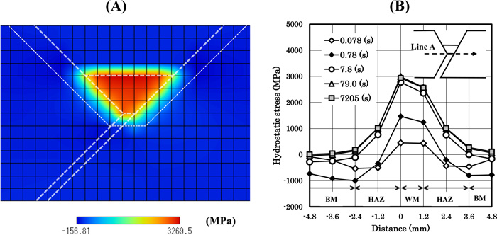
Figure 8 shows the hydrogen concentration distributions. Figures 8(A), 8(B), 8(C) and 8(D) show the distributions of 0 (s), 0.78 (s), 23.4 (s) and 7205 (s), respectively. Figure 8(A) shows the initial hydrogen distribution. At t=0.78 (s), most of hydrogen exists in the weld metal, and the concentration is very high. At t=23.4 (s), high hydrogen concentration is still recognized in some part of the weld metal. However, these high hydrogen concentrations are not detrimental because of the high temperatures. The hydrogen distribution in Fig. 8(D) is obviously lower than those of Figs. 8(A), 8(B) and 8(C). However, since the cooling process is completed, this distribution is very important. Figure 8(D) also shows the details of the hydrogen distribution in the HAZ and the weld metal. High hydrogen concentration regions in Fig. 8(D) are the HAZ and the weld metal near the weld root. The hydrostatic stress shown in Fig. 7(B) is the highest at the weld root. This is the reason why hydrogen concentration neat the weld root in Fig. 8(D) becomes high.

Fig. 8.

Transient changes of hydrogen concentration distributions. (A), (B), (C) and (D) show the distributions of 0 (s), 0.78 (s), 23.4 (s) and 7205 (s), respectively. The hardness values of the base metal, the HAZ and the weld metal are 360, 400 and 340, respectively. (Online version in color.)

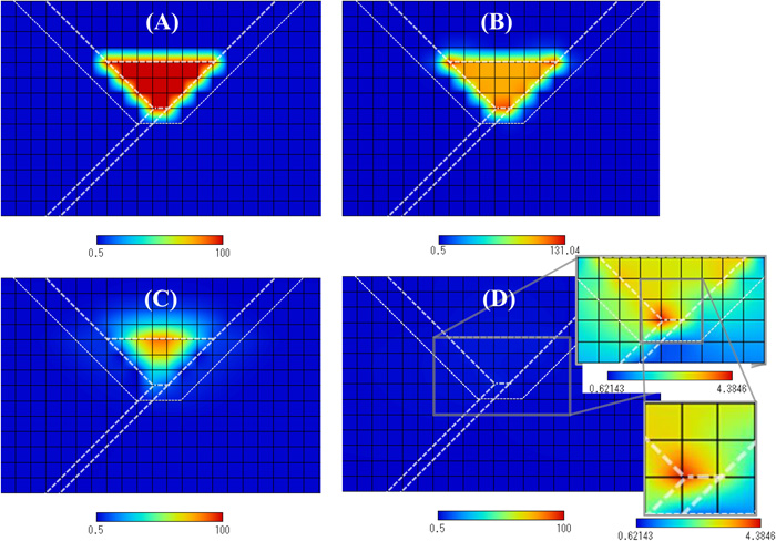
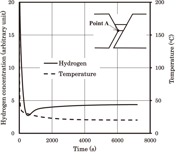
Figure 9 shows the time dependence of hydrogen concentration profile along line A. We can see that the hydrogen concentration at the weld root firstly decreases (7.8 (s) to 779.8 (s)) and turns to increase (779.8 (s) to 7205 (s)). Figure 10 shows the time dependences of temperature and hydrogen concentration at point A. Point A is defined as the point of the weld root on line A. Figure 10 shows the hydrogen accumulation occurs after the temperature becomes almost equal to the room temperature. Hydrogen concentration at early stage decreases rapidly, but turns to increase. This increase occurs when the cooling process is almost finished, and continues for several thousand of seconds. It seems that hydrogen concentration becomes almost constant after t=6000 (s). We would like to emphasize that this result has been obtained using the boundary condition of the surface obtained in the companion paper. As mentioned in the companion paper, the effect of the surface in the present model is very high, that is, the fast escape of hydrogen to the atmosphere. Nevertheless, the high hydrogen concentration near the weld root compared with the centre of the weld metal has been obtained. This is probably because of the stress driven term in Eq. (4). In order to avoid cold cracking, the steel and the welding consumable should have sufficient resistance to cold cracking under the condition of the hydrogen accumulation. Otherwise, the welding condition has to be changed, for example, higher weld heat input and so on.

Fig. 9.

Transient change of the hydrogen concentration distribution along line A. The hardness values of the base metal, the HAZ and the weld metal are 360, 400 and 340, respectively.

Fig. 10.

Time dependences of hydrogen concentration and temperature at point A. The hardness values of the base metal, the HAZ and the weld metal are 360, 400 and 340, respectively.

4.4. Results of the Even-match Case

Figure 11 shows the hydrostatic stress (σ_p) distributions. Figures 12 and 13 show the transient changes of the hydrogen concentration distributions. Figure 12 shows the distributions for 0 (s), 0.78 (s), 23.4 (s) and 7205 (s), and Fig. 13 shows the distributions along line A. Figure 14 shows the time dependences of hydrogen concentration and temperature at point A. At early stage, hydrogen concentration in Fig. 13 decreases more rapidly than that of Fig. 9. This may be because of the lower hardness values of the base metal and the HAZ. The lower hardness value results in higher D_app, and hence hydrogen can diffuse more easily. However, at t=7205 (s), hydrogen distribution along line A in Fig. 13 is very similar to that in Fig. 9. This is probably because of the stress driven term in Eq. (4). Actually, the hydrostatic stress distribution in Figs. 7(B) and 11(B) at the weld root are almost the same.

Fig. 11.

Hydrostatic stress distributions. (A) is of t=7205 (s), and (B) shows the profile along line A. The hardness values of the base metal, the HAZ and the weld metal are set to be 280, 320 and 340, respectively. (Online version in color.)

Fig. 12.

Transient changes of hydrogen concentration distributions. (A), (B), (C) and (D) show the distributions of 0 (s), 0.78 (s), 23.4 (s) and 7205 (s), respectively. The hardness values of the base metal, the HAZ and the weld metal are 280, 320 and 340, respectively. (Online version in color.)

Fig. 13.

Transient change of the hydrogen concentration distribution along line A. The hardness values of the base metal, the HAZ and the weld metal are 280, 320 and 340, respectively

Fig. 14.

Time dependences of hydrogen concentration and temperature at point A. The hardness values of the base metal, the HAZ and the weld metal are 280, 320 and 340, respectively.

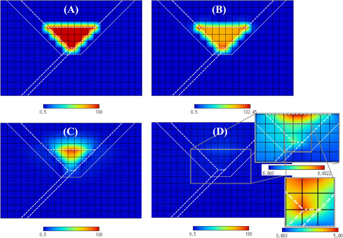
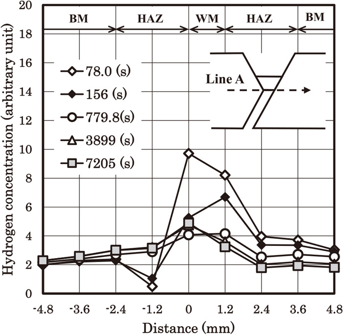
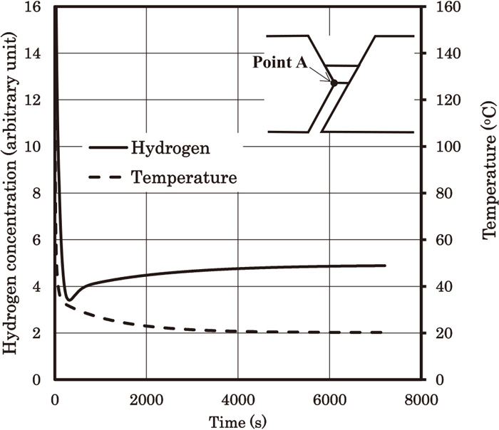
Figure 15 shows the hydrostatic stress distributions along line B. Line B is defined as a line passing through point A which is perpendicular to line A. Figure 15(A) is for the under-match case, and Fig. 15(B) is for the even-match case. The hydrostatic stress near the upper surface of the weld metal in both cases is relatively high, and the stress dependent terms in Eq. (4) tend to increase the hydrogen concentration near the surface. We can see this tendency in both Figs. 8(C) and 12(C). We can also recognize the same tendency in Fig. 12(D). However, contrary to Fig. 12(D), the hydrogen concentration near the surface in Fig. 8(D) is not relatively high. This difference may be caused by the difference in the gradient of D_app. In the under-match case, the Hv value of the weld metal is the lowest. The D_app value of the weld metal is hence the highest, and ∇D_app terms in Eq. (4) tend to make hydrogen diffuse from the weld metal to the HAZ. This tendency is opposite to that of the stress dependent terms. Which tendency is more dominant can be evaluated considering the numerical calculation results. In the even-match case, the Hv value of the weld metal is the highest, and hence the D_app value of the weld metal is the lowest. In this case, ∇D_app terms in Eq. (4) tend to make hydrogen diffuse from the HAZ to the weld metal. This tendency is the same as that of the stress dependent terms. So the hydrogen concentration near the surface of the weld metal in Fig. 12(D) is relatively high, and Fig. 12(D) indicates the weld metal cracking.

Fig. 15.

Transient change of the hydrostatic stress along line B. (A): the hardness values of the base metal, the HAZ and the weld metal are 360, 400 and 340, respectively. (B): the hardness values of the base metal, the HAZ and the weld metal are 280, 320 and 340, respectively.

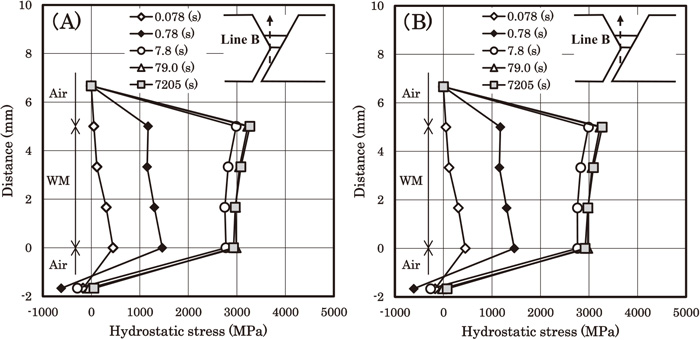
Figure 16 shows the equivalent plastic strain distributions of the two cases. Figure 16(A) is for the under-match case, and Fig. 16(B) is for the even-match case. We can see that the plastic strains in the weld metal, especially near the weld toes are relatively high. Such distribution of the plastic strain is considered to make D_app of the weld metal lower, which might result in the increase of hydrogen concentration in the weld metal. In the even-match case, this tendency of the plastic strain is the same as those of the hydrostatic stress and the hardness. In the under-match case, the tendency of the plastic strain is the same as that of the hydrostatic stress, but is opposite to that of the hardness. In the under-match case, we can recognize that the hydrogen concentration in the HAZ and the weld metal near the weld root is relatively high as shown in Fig. 8(D), and hence the effect of the hardness in the under-match case is considered higher than those of the hydrostatic stress and the plastic strain. The fact that this type of discussion can be conducted from the numerical calculations is a merit of the present model.

Fig. 16.

Equivalent plastic strain distributions at 7205 (s). (A): the hardness values of the base metal, the HAZ and the weld metal are 360, 400 and 340, respectively. (B): the hardness values of the base metal, the HAZ and the weld metal are 280, 320 and 340, respectively. (Online version in color.)

4.5. Comparisons with the Experimental Results

The calculation results of the under-match case in Fig. 8(D) show that high hydrogen concentration is recognized in the weld root (stress concentration area) of both the HAZ and the weld metal. The results of the even-match case in Fig. 12(D) show that, in addition to the hydrogen accumulation in the weld root, hydrogen concentration in the weld metal is also high. Since high hydrogen concentration means high cold cracking susceptibility, the results in Fig. 8(D) indicate that crack may be initiated at the weld root and propagate in the HAZ and/or in the weld metal. On the other hand, the results in Fig. 12(D) indicate that crack initiated at the weld root may propagate in the weld metal. The experimental result of the under-match case in Fig. 2 shows that crack firstly propagated in the HAZ along the fusion line and then went into the weld metal. This crack propagation path is in good agreement with Fig. 8(D). For the even-match case, we use the experimental data of Okamura et al.³⁾ Their result was the weld metal crack, and this result agrees with the general tendency reported by Matsuda et al.²⁾ Hence the calculation results in Fig. 12(D) fairly agree with the experimental results. The difference between Figs. 8(D) and 12(D) has been obtained by the difference in hardness distribution between the two cases. The present hydrogen diffusion model can consider the effect of hardness on D_app. In addition, the stress-strain curves were obtained considering the hardness values. The distribution of plastic strain is influenced by the hardness distribution, and hence the distribution of D_app is also influenced. However, it should be emphasized that other factors such as restraint intensity²²⁾ can also influence the distribution of plastic strain. The restraint intensity of the y groove weld cracking test is very high, and hence in the present work both sides of the specimen were restrained as shown in Fig. 6. We can simulate welded joints with lower restraint intensity by modifying the restraint condition. The present model can reflect these influences on the hydrogen diffusion calculations.

In general, the strength of weld metal is set to be equivalent to or sometimes higher than that of steel to ensure the strength of a welded joint. When their strengths are 780 MPa or over, cold crack tends to occur and propagate not in the HAZ but in the weld metal because there are a variety of the steel production processes such as quenched-tempered (QT) and thermo-mechanical control processes (TMCP). These processes can reduce the alloy elements of steel and consequently can reduce an index of cold cracking susceptibility such as P_CM.²³⁾ In the case of weld metal, its strength has to meet the requirement under the as-welded condition whose welding heat input is sometimes higher than that of the present cracking test. Hence the alloy elements in the weld metal are likely to increase, resulting in higher cold cracking susceptibility of the weld metal. Because of such characteristics, in the case of multi-pass welding, under-match welding consumables may be used for the first welding pass to avoid cold cracking in the weld metal. This procedure is considered adequate owing to the lower cold cracking susceptibility of the weld metal. The whole strength of the welded joint can be obtained using the even-match and/or over-match welding consumables for the subsequent welding passes. In this case, the risks that should be considered are of the HAZ cracking during the first welding pass and of the weld metal cracking during the subsequent passes. To evaluate these risks, the hydrogen diffusion analysis is important because the hydrogen distribution depends on the selection of the materials. And we consider the present model can give useful information. In addition, with the conventional hardness prediction methods,^6,19) it is expected that the present model can be applied to evaluate cold cracking susceptibility of a wide variety of high strength steel welded joints.

5. Conclusion

We conducted a y groove weld cracking test using 980 MPa grade steel and 780 MPa grade welding consumable. The crack firstly propagated in the HAZ and then went into the weld metal. The numerical calculations of the present hydrogen diffusion model show that relatively high hydrogen concentration is recognized in the weld root of the HAZ and the weld metal, which fairly agrees with the present experiment. We also conducted the numerical calculations of the cracking test with 780 MPa grade steel and 780 MPa grade welding consumable. In this case, in addition to the hydrogen accumulation in the weld root, relatively high hydrogen concentration is recognized in the weld metal, which indicates the weld metal cracking. The calculation results fairly agree with the experimental results in the literature. It is expected that the present hydrogen diffusion model is applicable to a wide variety of the high strength steel welded joints.

Acknowledgment

This work was partially supported by Council for Science, Technology and Innovation (CSTI), Cross-ministerial Strategic Innovation Promotion Program (SIP), “Structural Materials for Innovation” (Funding agency: JST), Japan.

References

• 1)  JIS Z 3158: 2016, Method of y-groove weld cracking test.
• 2)   F.  Matsuda,  H.  Nakagawa,  K.  Shinozaki and  Y.  Sanematsu: Q. J. Jpn. Weld. Soc., 5 (1987), 94 (in Japanese). https://doi.org/10.2207/qjjws.5.94
• 3)   Y.  Okamura,  M.  Tanaka,  M.  Okushima,  R.  Yamaba,  H.  Tamehiro,  H.  Inoue,  T.  Kasuya and  A.  Seto: Nippon Steel Tech. Rep., 66 (1995), 65. https://www.nipponsteel.com/en/tech/report/nsc/pdf/6608.pdf
• 4)   N.  Itakura,  K.  Yasuda and  M.  Aoki: Kawasaki Steel Giho, 30 (1998), 174 (in Japanese). https://www.jfe-steel.co.jp/archives/ksc_giho/30-3/j30-174-180.pdf
• 5)  AWS A5.5/A5.5M: 2006, Specification for low-alloy steel electrodes for shielded metal arc welding.
• 6)   N.  Yurioka,  M.  Okumura,  T.  Kasuya and  H. J. U.  Cotton: Met. Constr., 19 (1987), 217R.
• 7)   A.  Alvaro,  V.  Olden,  A.  Macadre and  O. M.  Akselsen: Mater. Sci. Eng. A, 597 (2014), 29. https://doi.org/10.1016/j.msea.2013.12.042
• 8)   A. T.  Yokobori, Jr.,  T.  Ohmi,  T.  Murakawa,  T.  Nemoto,  T.  Uesugi and  R.  Sugiura: Strength, Fract. Complex., 7 (2011), 215. https://doi.org/10.3233/SFC-2011-0140
• 9)   A. T.  Yokobori, Jr.,  T.  Nemoto,  K.  Satoh and  T.  Yamada: Eng. Fract. Mech., 55 (1996), 47. https://doi.org/10.1016/0013-7944(96)00002-1
• 10)   A. T.  Yokobori, Jr.,  Y.  Chinda,  T.  Nemoto,  K.  Satoh and  T.  Yamada: Corros. Sci., 44 (2002), 407. https://doi.org/10.1016/S0010-938X(01)00095-6
• 11)   J. B.  Leblond and  D.  Dubois: Acta Metall., 31 (1983), 1459. https://doi.org/10.1016/0001-6160(83)90142-6
• 12)   A.  McNabb and  P. K.  Foster: Trans. Metall. Soc. AIME, 227 (1963), 618.
• 13)   H. P.  Van Leeuwen: Eng. Fract. Mech., 6 (1974), 141. https://doi.org/10.1016/0013-7944(74)90053-8
• 14)   G.  Ozeki,  A. T.  Yokobori, Jr.,  T.  Ohmi,  T.  Kasuya,  N.  Ishikawa,  S.  Minamoto and  M.  Enoki: Adv. Mater. Lett., 9 (2018), 677. https://doi.org/10.5185/amlett.2018.2160
• 15)   G.  Ozeki,  A. T.  Yokobori, Jr.,  T.  Ohmi,  T.  Kasuya,  N.  Ishikawa,  S.  Minamoto and  M.  Enoki: Proc. ASME 2018 Pressure Vessels and Piping Conf., (Prague), ASME, New York, (2018), PVP2018-84178. https://doi.org/10.1115/PVP2018-84178
• 16)   A. T.  Yokobori, Jr.,  G.  Ozeki,  T.  Ohmi,  T.  Kasuya,  N.  Ishikawa,  S.  Minamoto and  M.  Enoki: Mater. Trans., 60 (2019), 222. https://doi.org/10.2320/matertrans.ME201716
• 17)   T.  Kasuya and  N.  Yurioka: Weld. J., 72 (1993), 107s. https://app.aws.org/wj/supplement/WJ_1993_03_s107.pdf
• 18)   Y.  Mikami,  N.  Kawabe,  N.  Ishikawa and  M.  Mochizuki: Q. J. Jpn. Weld. Soc., 34 (2016), 67 (in Japanese). https://doi.org/10.2207/qjjws.34.67
• 19)   T.  Kasuya and  Y.  Hashiba: Sci. Technol. Weld. Join., 4 (1999), 265. https://doi.org/10.1179/136217199101537851
• 20)   H. F.  Jackson,  C.  San Marchi,  D. K.  Balch and  B. P.  Somerday: Corros. Sci., 77 (2013), 210. https://doi.org/10.1016/j.corsci.2013.08.004
• 21)   Y.  Yamada: Sosei-Nendansei (Plasticity·Viscoelasticity), Baifukan, Tokyo, (1977), 173 (in Japanese).
• 22)   K.  Satoh: J. Jpn. Weld. Soc., 30 (1961), 212 (in Japanese). https://doi.org/10.2207/qjjws1943.30.212
• 23)   Y.  Ito and  K.  Bessyo: J. Jpn. Weld. Soc., 37 (1968), 983 (in Japanese). https://doi.org/10.2207/qjjws1943.37.983