Approximation and Characteristic Times in Precipitation Modelling

Abstract

A new approximation to the equations describing Classical Nucleation and Growth Theories, is proposed providing quick, and intuitive insight. It gives a prediction of the mean precipitate radius and number density development under quasi-isothermal conditions. Current “mean-radius”, and “multi-class” approaches to modelling classical nucleation and growth theory for precipitation, require considerable computation times. An analytical approximation is proposed to solve the equations, and its results are compared to numerical simulations for quasi-isothermal precipitation. From the approximation a start and end time for the nucleation stage is predicted, as well as a time at which growth occurs and when the coarsening stage starts. Ultimately, these times, outline the numerical solution to the precipitation trajectory, providing key insight before performing numerical simulations. This insight can be used to more efficiently simulate precipitate development, as time scales at which the various stages in precipitate development occur can be predicted for individual precipitates. When these time scales are known a numerical simulation can be used for a specific goal, for instance to only simulate nucleation and growth, thus saving computational time. Moreover, for a first indication of the precipitate development in a composition under a particular heat treatment a numerical simulation is no longer necessary. This is also useful for process control as consequences of changes in treatment can be assessed on-line. Using these approximate analytical results an estimate can be made for the matrix concentration of precipitate forming elements. Additionally some dimensionless parameters are established to provide intuitive details to the precipitation trajectory.

1. Introduction

Precipitation of a second solid phase from solid solution is commonly used to enhance metal alloy properties. An example of this enhancement is grain size control in low alloyed steel,¹⁾ another example is precipitation hardening.^{2,3,4,5,6,7,8)} Many models exist to model the precipitate development under given processing treatment, e.g.,^{2,9,10,11,12)} The goal of modelling precipitation is to establish the relation between processing parameters and the evolution of the precipitate sizes and precipitate volume fraction.

Different types of models exist to simulate the precipitate size and number density evolution during heat treatment. One commonly used type is based on Classical Nucleation and Growth Theory (CNGT) models.¹³⁾ CNGT precipitation models can be divided into two approaches; (i) mean-radius approach; and (ii) multi-class approach. In some cases both approaches return the same result, but in more complex systems and/or process conditions the results can differ and the more sophisticated multi-class models are required.¹³⁾ Unfortunately multi-class models require much more computational resources than mean-radius models, which matters particularly for more complex systems.

With growing computational power current research is focussed on expanding the accuracy and applicability of CNGT models, e.g.,^12,14,15,16) however this does not provide any detailed intuitive insight in the precipitation trajectory. This paper seeks to provide a fast analytical approximation to quasi-isothermal precipitation for one precipitate type at one site, and from this approximation derive parameters which provide a more intuitive insight into the development of the precipitates. Though only one type of precipitate can be assessed at one nucleation site, results for multiple types and sites can be compared quickly. Allowing prediction of which precipitate will form first and where.

The approximation method is illustrated in section 2.3 using an idealised system, defined by isothermal conditions, one type of precipitate, one type of nucleation site, and all available nucleation sites are assumed to be occupied. The approximation can only be applied to a single phase matrix, so interphase precipitation is not considered. Using this approximation several parameters are defined, which characterize the precipitate evolution, thus providing a more intuitive insight into the simulated precipitate development. As a second step, the restriction that all nucleation sites are occupied is relaxed in section 2.7, and a new approximation is derived for the case that the maximum precipitate number density is lower than the maximum available nucleation sites per unit of volume. Finally the isothermal condition is relaxed in section 3 and replaced by a quasi-isothermal approximation for non-isothermal conditions. Examples for this most generalized approximation are presented. Section 4 gives a discussion of the validity and limitations of the methods, which are here presented.

2. Derivation for Isothermal Precipitation

2.1. Evolution Equations

The rate of change for the precipitate number density distribution ϕ(R,t), where t is the time, and R the radius of the precipitate, is given by (cf. Hulburt and Katz¹⁷⁾):   

$$\frac{\partial \varphi }{\partial t}=-\frac{\partial \left[\left(\partial R/\partial t\right)\varphi \right]}{\partial R}+\frac{\partial N}{\partial t}\delta \left(R-R^{*}\right),$$(1)

where N is the precipitate number density, R^* is the critical radius, and δ is the Dirac-delta function. It may be noted that the precipitate number density N(t) is the 0-th moment of ϕ(R,t),   

$$N\left(t\right)={\int }_0^{\infty }\varphi \left(R,t\right)dR,$$(2)

Solving Eq. (1) is an arduous task due to the non-linear nature of the right-hand-side of the equation. In the right-hand-side of Eq. (1) a nucleation rate and a growth rate for existing precipitates are included. The nucleation rate is given by:^18,19,20)   

$$\frac{\partial N}{\partial t}=\left(N_{\text{total}}-N\right)Z{\beta }^{*}\text{exp}\left(-\frac{\mathrm{\Delta }{G}^{*}}{k_{B}T}\right),$$(3)

where Z is the Zeldovich factor,¹⁹⁾ β^* the condensation rate,²⁰⁾ and ΔG^* the activation energy,¹⁸⁾ the energy required to form a nucleus. N_total is the number of available nucleation sites, k_B is the Boltzmann constant, and T the absolute temperature. Note that the form of the activation energy, ΔG^*, depends on the nucleation site. The results of this work are, however, not site dependent, as they do not depend on the specific form of the activation energy. A steady-state nucleation rate is used, as under normal circumstances incubation time^2,21) τ_inc = 1/(2Z²β^*) is considerably smaller than the time-scales found in this work. For AlN precipitation in austenite on grain boundaries similar results are found, not reported here. The effect of an incubation time is therefore considered negligible for the results of this work, for further comments regarding incubation time see section 2.5.

For the growth rate of precipitates the mean value approximation is used here, in which the Gibbs-Thomson effect is included to account for the interfacial energy between precipitate and matrix (which enters through $C_m^{\overline{R}}$, cf.²⁾). The growth rate for the average radius, $\overline{R}$, is given by:^2,22)   

$$\frac{\text{d}\overline{R}}{\text{d}t}=\frac{D_{\text{eff}}}{\overline{R}}\frac{C_m- C_m^{\overline{R}}}{C_m^P-C_m^{\overline{R}}}+\frac{1}{N}\frac{\partial N}{\partial t}\left(\alpha R^{*}-\overline{R}\right),$$(4)

here D_eff is the effective diffusivity for the given nucleation site. An example for the effective diffusivity concerning precipitation on dislocations is given by Dutta and Sellars.¹⁰⁾ Furthermore, for the growth rate there are three important concentrations for each element m in the system;¹²⁾ $C_m^P$ inside the precipitate, $C_m^{\overline{R}}$ at the precipitate-matrix interface at the matrix side, and C_m the matrix concentration of element m. The growth rate of Eq. (4), is used for “mean-radius” models, where the first term accounts for the growth of existing particles, and the second term for the newly nucleated particles. α ensures that precipitates that are slightly larger than the critical radius can grow, Deschamps et al.²⁾ use α=1.05. In this work the nucleation correction is assumed to be negligible as the highest growth rate generally occurs after the nucleation stage has finished, the growth rate is therefore taken as^†:   

$$\frac{\text{d}\overline{R}}{\text{d}t}=\frac{D_{\text{eff}}}{\overline{R}}\frac{C_m- C_m^{\overline{R}}}{C_m^P-C_m^{\overline{R}}}.$$(5)

Cases where the nucleation correction cannot straightforwardly be neglected are studied more closely in section 2.7, where it is shown that this assumption is still usable. For the interface concentration $C_m^{\overline{R}}$ the description from Deschamps²⁾ is used:   

$$\begin{array}{l}{C}_m^{\overline{R}}=C_m^{eq}\text{exp}\left(\frac{R_0}{\overline{R}}\right),R_0\equiv R^{*}\text{ln}\left(C_m/C_m^{eq}\right)\equiv \frac{2\gamma v_{\text{mol}}}{R_{\text{gas}}T}\\ \Rightarrow C_m^{\overline{R}}=C_m^{eq}\left({\left[\frac{C_m}{C_m^{eq}}\right]}^{\frac{R^{*}}{\overline{R}}}\right),\end{array}$$(6)

where R₀ is defined to include the Gibbs-Thomson effect, v_mol is the molar volume of the precipitate, R_gas is the gas constant, γ is the matrix-precipitate interface energy, and $C_m^{eq}$ is the equilibrium matrix concentration. Solving Eq. (5) becomes notably harder when the Gibbs-Thomson effect is included, which is radius-dependent. Additionally, for common precipitates under regular heat treatment conditions, the Gibbs-Thomson effect typically yields $C_m^{\overline{R}}\le 3C_m^{eq}$ for nanometre-size particles using common parameter values. The effect is further reduced when particles grow larger. The surface concentration is therefore replaced by the equilibrium concentration, and Eq. (5) is rewritten to:   

$$\frac{\text{d}\overline{R}}{\text{d}t}=\frac{D_{\text{eff}}}{\overline{R}}\frac{C_m- C_m^{eq}}{C_m^P-C_m^{eq}}.$$(7)

This is the growth rate for the average radius that will be used in this work. Note that, for both Eqs. (3) and (7), the right-hand-side is generally time-dependent.

^†  This form is identical to the expression for individual particles in the distribution form of Eq. (1): $dR/dt=D_{\text{eff}}/R\left(C_m-C_m^R\right)/\left(C_m^P-C_m^R\right)$, see Den Ouden.¹²⁾

2.2. Reference Model

The proposed approximation is compared to a multi-class KWN-model as specified by Den Ouden,¹²⁾ which has been encoded in Matlab, and for which the governing equations have been given in section 2.1. The Den Ouden model is an improved version of the model proposed by Robson.²¹⁾ In this work it shall be used to simulate the development of a single type of precipitate, but the model allows for multiple types of precipitates to develop simultaneously. The original KWN model only considered homogeneous precipitation, and therefore in order to model precipitate formation on dislocations an adaptation of the model proposed by Zurob⁹⁾ was included in the Den Ouden model. Additionally, precipitation on grain boundaries was included.

Throughout this work focus shall be on steel of one chemical composition; Fe 98.4695%, Mn 1.34%, Si 0.06%, Nb 0.03%, Al 0.01%, C 0.076%, N 0.0061%, P 0.0058%, and S 0.0026% by weight.

The precipitate that is studied is niobium carbide (NbC). The suggested approximations in this work are applied to the general equations, therefore they are equally valid for other precipitates. Only nucleation at dislocations is considered, however different sites can be approximated for by altering the relevant parameters in Eqs. (3) and (4). The activation energy for nucleation at dislocations is found from ΔG(R)=VΔG_V+Aγ−μb²R$\left(\text{ln}\left(\raisebox{1ex}{$R$}\!\left/ \!\raisebox{-1ex}{$b$}\right.\right)/\left(2\pi \left(1-\nu \right)\right)-1/5\right)$, following Zurob et al.^9,23,24) The parameters used for NbC are listed in Table 1:

Table 1. Model parameters used in the reference simulations. Here T is given in Kelvin, and R_gas is the universal gas constant in J K⁻¹ mol⁻¹. For the solubility product the concentrations used are in wt%.

Name		Value	Unit
Interface energy [NbC]	γ	1.0058−0.4493·10−3T	Jm−2
Molar volume [NbC]9)	vmol	13.39·10−6	m3mol−1
Bulk diffusivity [Nb]9)	Dbulk	$0.83\cdot {10}^{-4}\cdot e^{-266\mathrm{\hspace{0.17em} }500/\left(R_{\text{gas}}T\right)}$	m2s−1
Pipe diffusivity [Nb]9)	Dpipe	$4.1\cdot {10}^{-4}\cdot e^{-172\mathrm{\hspace{0.17em} }500/\left(R_{\text{gas}}T\right)}$	m2s−1
Solubility prod. [NbC]25)	Ksol	103.42−7900/T	–
Dislocation density	ρ	3.27·1014	m−2
Burgers vector	b	2.53144·10−10	m
Correction factor9)	F	1.32·10−3	–
Poisson ratio9)	ν	0.293	–
Shear modulus9)	μ	$81 -\frac{73.71\left(T-300\right)}{1\mathrm{\hspace{0.17em} }810}$	GPa

The correction factor F is used in the reference model and was defined by Zurob et al.,⁹⁾ where F is used to fit the model to experimental data. The value in this work was fitted in-house for the reference model, and is comparable to the value presented by Zurob et al.⁹⁾ F typically has an order of magnitude F~1·10⁻³ to 1·10⁻², as it can be viewed as the average spacing between nucleation sites along a dislocation line as a multiple of the Burgers vector. The practical use of F is to determine the number of nucleation sites for precipitates at dislocations, N_total=Fρ/b.⁹⁾

2.3. First Approximation

Our method for approximation is illustrated by starting from a simplified system:

1. The system is isothermal during the entire process.

2. Only precipitates of one composition are considered.

3. Only one type of nucleation site is considered, i.e., only homogeneous, or on dislocations, or on grain boundaries.

4. At the start of the process there are no precipitates, i.e., only the initial stage of precipitation is considered in the first approximation of this work.

5. At the end of the nucleation stage all the available sites for nucleation are occupied, i.e., the maximum number density is attained.

6. The matrix exists as a single phase, so no interphase precipitation occurs.

7. The incubation time is small with respect to the characteristic nucleation time defined below, i.e., ${\tau }_{\text{inc}}\ll {\tau }_{\eta }$.

Both Eqs. (3) and (7) are non-linear differential equations. To approximate solutions for both equations they are rewritten for notational convenience:   

$$\frac{\partial N}{\partial t}=\left(N_{\text{total}}-N\right)Z{\beta }^{*}\text{exp}\left(-\frac{\mathrm{\Delta }{G}^{*}}{k_{B}T}\right)\equiv \frac{N_{\text{total}}-N}{{\tau }_{\eta }\left(t\right)},$$(8)

and   

$$\frac{\text{d}\overline{R}}{\text{d}t}=\frac{D_{\text{eff}}}{\overline{R}}\frac{C_m- C_m^{eq}}{C_m^P-C_m^{eq}}\equiv \frac{\mathrm{\Sigma }\left(t\right)}{\overline{R}}.$$(9)

Where the (explicitly) time-dependent parameters ${\tau }_{\eta }\left(t\right)=\text{exp}\left(\frac{\mathrm{\Delta }{G}^{*}}{k_{B}T}\right)/Z{\beta }^{*}$ and $\mathrm{\Sigma }\left(t\right)=D_{\text{eff}}\frac{C_m- C_m^{eq}}{C_m^P-C_m^{eq}}$ are defined.

Under the listed restrictions it is assumed that both τ_η(t) and Σ(t) can be considered time-independent. This may be done as external variables like temperature are constant, and only a single composition of precipitate is considered at a specific site. The approximation essentially assumes that the matrix concentration will not change too much. Now both equations reduce to ordinary differential equations.

When τ_η(t)=τ_η(0)≡τ_η and Σ(t)=Σ(0)≡Σ, i.e., are time-independent, Eq. (8) resolves to:   

$$N\left(t\right)=N_{\text{pre}}+\left(1-\text{exp}\left(-\frac{t}{{\tau }_{\eta }}\right)\right)\left(N_{\text{total}}-N_{\text{pre}}\right),$$(10)

where N_pre is the pre-existing number density, under the given restrictions N_pre=0. And for Eq. (9):   

$$\overline{R}\left(t\right)=\sqrt{2\mathrm{\Sigma }t+{\left(\overline{R}\left(0\right)\right)}^2}.$$(11)

Here $\overline{R}$(0)=R^*, R^* is the critical radius which is constant under the used restrictions.

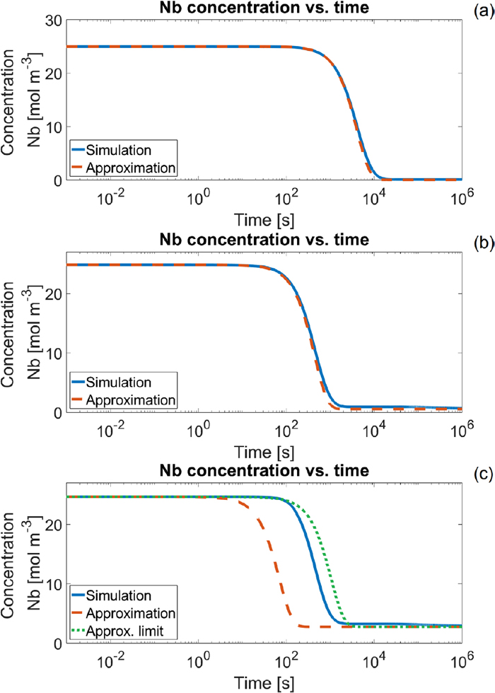
Some examples of calculations are presented in Fig. 1. The approximation for precipitate number density agrees with the simulated number density from the KWN model; in the case that all the available sites are occupied. The number of available sites for dislocation precipitates is found from Fρ/b.⁹⁾ The values of these three parameters are given in Table 1. The agreement between the approximation and the simulation result can be seen in Figs. 1(b) and 1(d), in these examples τ_η = 4.6, 1.9, 3.5·10² s in the order of ascending temperature. Therefore it is worthwhile to determine when the nucleation stage starts and when it ends following Eq. (10). The true start and end of nucleation are at the limits t = 0 and t = ∞ respectively, so a threshold value is chosen for the start when 5% of the sites are occupied, and for the end of nucleation when 95% of the sites are occupied. These times will be labelled t_5% and t_95% respectively, and are found to be:   

$$t_{5\%}=ln\left(20/19\right){\tau }_{\eta }=0.05{\tau }_{\eta },\hspace{1em}{t}_{95\%}=ln\left(20\right){\tau }_{\eta }=2.996{\tau }_{\eta }.$$(12)

These ‘nucleation’ times provide an intuitive insight into the time interval during which nucleation plays its role in the precipitate development. Note that the quotient of t_95% and t_5% is a dimensionless constant t_95%/t_5% = 58.4, because of the idealised nature of the approximation. Furthermore, when t_95% is large compared to the time-scales associated with growth, the matrix concentration is likely to change significantly before all nuclei have formed. Then the initial assumption that τ_η is time-independent is likely to be invalid, this condition is discussed in section 2.4.

Fig. 1.

Average radius and number density respectively of the NbC precipitates under isothermal conditions at 650°C in (a) and (b), at 750°C in (c) and (d), and at 850°C in (e) and (f). The blue solid line shows the results of the reference multi-class KWN model by Den Ouden¹²⁾ are given. The red dashed line represents the approximations from Eqs. (10) and (11) for the number density and average radius respectively are given. For the average radii (cf. (a), (c), and (e)) the bootstrapping results from Eq. (19) are given in the dotted green line, while the purple dash-dotted line is the average radius following LSW theory,^26,27) see Eq. (23). For the number density (cf. (b), (d), and (f)) the purple dash-dotted line represents the number density following the LSW theory, Eq. (25). Additionally the black (horizontal) dashed lines (in (b), (d), and (f)) represent the maximum number of nucleation sites per unit volume. In (f) not all available sites are occupied, additional input is required to capture this as well, which is presented in section 2.7. (Online version in color.)

2.4. Bootstrapping and Approximating Matrix Concentration

Equations (10) and (11) are rather rough approximations; once the matrix concentration is changing due to growing precipitates the approximation breaks down, because especially the activation energy ΔG^* in the exponent of the nucleation equation, (Eq. (3)) is sensitive for changes in the concentration.¹⁸⁾ To overcome this limitation ‘bootstrapping’ is performed: this bootstrapping implies substituting the previous approximations to the average size and number density. The matrix concentration, and the mass conservation law are suitable equations for this substitution. Essentially a one-step iteration is performed based on previous results.

Bootstrapping applied to the evolution of the matrix concentration also leads to the derivation of a second characteristic time τ_λ from the changing matrix concentration:   

$$\frac{\text{d}}{\text{d}t}\left[C_m\right]=\frac{\text{d}}{\text{d}t}\left[C_m^{\text{init}}-\frac{4\pi \left(C_m^P-C_m^{\text{init}}\right)}{3}\left(N{\overline{R}}^3\right)\right],$$(13)

here $C_m^{\text{init}}$ is the initial concentration of m, Eq. (13) returns:   

$$\frac{\text{d}{C}_m}{\text{d}t}=-\frac{4\pi \left(C_m^P-C_m^{\text{init}}\right)}{3}\left(3N\left(t\right){\overline{R}}^2\left(t\right)\frac{\text{d}\overline{R}}{\text{d}t}+{\left({\overline{R}}^{*}\right)}^3\frac{\text{d}N}{\text{d}t}\right).$$(14)

To approximate a solution for this equation some simplifications are made. First the loss of over-saturation by the newly nucleating precipitates is neglected. This may be done as the nucleation rate is high at the start of nucleation, where R^* is small, i.e., the product (R^*)³(dN/dt) is small, so a negligible amount of the solute over-saturation is consumed. When the concentration in the matrix decreases, the critical radius will increase, but the nucleation rate will also decrease. So in fact it is assumed that the over-saturation mainly decreases due to precipitate growth. As an additional assumption this growth will mainly take place when the precipitate number density has reached the maximum available number of nucleation sites, N_total. In section 2.7 this last assumption will be relaxed. So instead of using N(t) it is substituted with N_total. Equations (9) and (11) can be substituted into Eq. (14) to give:   

$$\begin{array}{l}{\displaystyle \frac{\text{d}{C}_m}{\text{d}t}}=-4\pi \left(C_m-C_m^{eq}\right){\displaystyle \frac{\left(C_m^P-C_m^{\text{init}}\right)N_{\text{total}}{D}_{\text{eff}}}{\left(C_m^P-C_m^{eq}\right)}}\\ \sqrt{2D_{\text{eff}}{\displaystyle \frac{C_m^{\text{init}}-C_m^{eq}}{C_m^P-C_m^{eq}}}}\sqrt{t}=-4\pi \left(C_m-C_m^{eq}\right){\displaystyle \frac{\sqrt{t}}{{\tau }_{\lambda }{}^{3/2}}},\end{array}$$(15)

where ${\tau }_{\lambda }={\displaystyle \frac{\left(C_m^P-C_m^{eq}\right)}{{\left[\left(C_m^P-C_m^{\text{init}}\right)N_{\text{total}}\right]}^{{\displaystyle \frac{2}{3}}}{D}_{\text{eff}}{\left(2C_m^{\text{init}}-2C_m^{eq}\right)}^{{\displaystyle \frac{1}{3}}}}}$, is time-independent by virtue of the earlier restrictions and assumptions. Equation (15) can be solved to yield:   

$$C_m\left(t\right)=\left(C_m^{\text{init}}-C_m^{eq}\right)\text{exp}\left(-\frac{2}{3}{\left[\frac{t}{{\tau }_{\lambda }}\right]}^{3/2}\right)+C_m^{eq}.$$(16)

Here it was assumed that for t = 0, C_m(0) = $C_m^{\text{init}}$. In Fig. 2 the results are shown for NbC precipitates under isothermal conditions.

Fig. 2.

The time evolution of the matrix concentration of Nb under isothermal conditions, at 650°C in (a), 750°C in (b) and at 850°C in (c). The solid blue lines represent the simulated matrix concentration, and the red dashed lines the approximation from Eq. (16). In (c) the green dotted line uses an alternate value for N_total, namely N_max see Eq. (28). (Online version in color.)

From the analytical expression in Eq. (16) it is also possible to define a start and end time, in a similar fashion as with the nucleation times in Eq. (12). The starting-time, t_g,5%, is defined as the time at which the difference between $C_m^{\text{init}}$ and $C_m^{eq}$ (the initial over-saturation) has decreased by 5%. The end-time, t_g,5%, is defined as the time at which the consumption of solute over-saturation has more-or-less ended, which is when the initial over-saturation has decreased by 95%,   

$$\begin{array}{l}{t}_{g,5\%}={\left[-\frac{3}{2}ln\left(\frac{19}{20}\right)\right]}^{2/3}{\tau }_{\lambda }=0.18{\tau }_{\lambda },\\ t_{g,95\%}={\left[-\frac{3}{2}ln\left(\frac{1}{20}\right)\right]}^{2/3}{\tau }_{\lambda }=2.72{\tau }_{\lambda }.\end{array}$$(17)

These times form good indicators for when the assumption that τ_η and Σ are time-independent loses its validity, as they tell how much the initial over-saturation has decreased, which is implicitly assumed to be constant. As with the nucleation times the quotient is also a dimensionless constant, t_g,95%/t_g,5% = 15.05. Using Eq. (16) an improvement can be made to Eq. (9). A time-dependence is added to Eq. (9) by substituting Eq. (16). The new expression reads:   

$$\frac{\text{d}\overline{R}}{\text{d}t}=\frac{D_{\text{eff}}}{\overline{R}}\frac{C_m^{\text{init}}- C_m^{eq}}{C_m^P-C_m^{eq}}\text{exp}\left(-\frac{2}{3}{\left[\frac{t}{{\tau }_{\lambda }}\right]}^{3/2}\right).$$(18)

Now Eq. (18) can be solved to return an improved solution to the average radius development over Eq. (11),   

$$\overline{R}\left(t\right)=\sqrt{\frac{\mathrm{\Sigma }{12}^{2/3}}{3}{\tau }_{\lambda }\left[\mathrm{\Gamma }\left(\frac{2}{3}\right)-\mathrm{\Gamma }\left(\frac{2}{3},\frac{2}{3}{\left[\frac{t}{{\tau }_{\lambda }}\right]}^{3/2}\right)\right]+{\left(\overline{R}\left(0\right)\right)}^2}.$$(19)

Where Γ(x) is the gamma-function, and Γ(x,y) is the upper incomplete gamma-function. The result is also shown in Figs. 1(a), 1(c), and 1(e) (dotted lines). In the worked-out examples the same plateau as with the simulated result shows up, at roughly the same time. This finite limit for the average radius is due to the asymptotic behaviour of the upper incomplete gamma function. The asymptotic behaviour is the result of the use of the average radius, and the assumption that the over-saturation is completely consumed in the growth stage by the precipitates. The improved approximation then suggests an average radius at which the nucleation and growth stage ends before coarsening starts.

The average radius right before coarsening is an important value, since it provides information as to what the maximum Zener pinning would be. This follows as the Zener pinning is proportional to the ratio of the volume fraction and the average radius. At the start of coarsening the maximum volume fraction is reached approximately, so the smaller the average radius at which this volume fraction is reached the higher the Zener pinning.

Now τ_η and τ_λ have been defined, they can both be used as characteristic times for nucleation and growth respectively. Under the restrictions given in section 2.3 ${\tau }_{\lambda }\gg {\tau }_{\eta }$, this indicates that the loss of over-saturation becomes only significant after nucleation has virtually stopped. The form of Eqs. (10) and (16) provides a handle on how far the nucleation or decrease in over-saturation has progressed, after τ_η units of time ≈ 63.2% of the maximum number density is reached, similarly after 3/2^2/3τ_λ units of time ≈ 63.2% of the over-saturation has been consumed by the precipitates. When τ_λ ≤ τ_η the approximations that were made need corrections to be able to provide a useful result. This is analysed in section 2.7.

2.5. Incubation Time

Some additional remarks must be made regarding the incubation time τ_inc. The incubation time has been considered negligible in this work as in many cases ${\tau }_{\text{inc}}\ll {\tau }_{\eta }$. However when τ_inc is comparable to τ_η it cannot be neglected. When it is included in Eq. (8) as found in literature^2,21) the solution becomes more complicated and much less intuitive than the result presented in Eq. (10). Additionally, the approximate result derived here becomes less accurate. However, when τ_inc ~ τ_η it is possible to still use Eq. (10) by shifting time by τ_inc. This shift can be used when nucleation is relatively quick compared to growth, see section 2.7. The predicted average radius and matrix concentration, may be shifted in time similarly. The use of this shift has been verified, results are not presented here as it can easily be verified by the reader. Note that when τ_inc ~ τ_λ and τ_inc ≥ τ_η one cannot neglect incubation time nor shift the approximations as described above because then nucleation and loss of over-saturation interfere.

However in this work, recall the timescale for nucleation τ_η is given as τ_η = 1/(Zβ^*exp(−ΔG^*/(k_BT))), and for consumption of over-saturation τ_λ goes with τ_λ ~ 1/((N_total)^2/3D_eff). It may be noted that these times as well as τ_inc increase when temperature, dislocation density, or diffusivity decrease, and vice-versa, albeit at a different rate for each timescale. In particular note that τ_inc/τ_η = exp(−ΔG^*/(k_BT))/Z, which has an absolute maximum in the domain T = [0,∞). When at this maximum ${\tau }_{\text{inc}}\ll {\tau }_{\eta }$, the incubation time can be neglected. In the examples of section 2.3 the maximum is at τ_inc/τ_η ≈ 2.2·10⁻³ at T ≈ 670°C, so incubation time can safely be neglected. Alternatively in the examples of section 2.3 in the order of ascending temperature, i.e., 650°C, 750°C, 850°C we find Z = 0.38, 0.19, 0.07 and β^* = 3.6·10², 6.3·10³, 1.0·10⁵ s⁻¹ with the incubation times τ_inc = 9.7·10⁻³, 2.3·10⁻³, 9.6·10⁻⁴ s. And τ_λ = 2.4·10⁵, 2.7·10⁴, 4.3·10³ s, so incubation time is not significant for the results presented here.

2.6. Coarsening

The approximate solutions derived so far only consider nucleation and growth. As shown in Fig. 1, coarsening in this approximation cannot be included, because the mean particle size only is considered. However, it is possible to use the LSW theory^26,27) for this purpose. The LSW theory solves the precipitate size distribution of Eq. (1) in the coarsening limit, and gives a description of the precipitate growth during coarsening. The resulting curve for the examples mentioned before can be found in the purple dash-dotted lines in Fig. 1, where the coarsening growth rate found in Eq. (22) is plotted from t = 0. When coarsening occurs in the simulation, the LSW theory and the simulation outcome follow the same curve, i.e., have the same time-dependence. Coarsening must be modelled explicitly for the mean-radius approach:²⁾   

$$\frac{\text{d}\overline{R}}{\text{d}t}=\frac{4}{27}\frac{C_m^{eq}}{C_m^P-C_m^{eq}}\frac{D_{\text{eff}}}{{\overline{R}}^2}\frac{2\gamma v_{\text{mol}}}{R_{\text{gas}}T}.$$(20)

For clarity Ω is defined as:   

$$\mathrm{\Omega }=\frac{4}{27}\frac{C_m^{eq}}{C_m^P-C_m^{eq}}{D}_{\text{eff}}\frac{2\gamma v_{\text{mol}}}{R_{\text{gas}}T}.$$(21)

This can be solved as an ordinary differential equation,   

$$\begin{array}{l}\overline{R}\left(t\right)={\left[3\mathrm{\Omega }t\right]}^{1/3}+{\overline{R}}_1\Rightarrow \overline{R}\left(t\right)\\ ={\left[\frac{4}{9}\frac{C_m^{eq}}{C_m^P-C_m^{eq}}\frac{2\gamma v_{\text{mol}}}{R_{\text{gas}}T}{D}_{\text{eff}}\right]}^{1/3}{t}^{1/3}+{\overline{R}}_1.\end{array}$$(22)

Where ${\overline{R}}_1$ is the radius at the start of coarsening,²⁶⁾ provided that Eq. (22) starts at coarsening, alternatively one can use the asymptotic value from Eq. (19). LSW theory is only valid on large time-scales, i.e., when coarsening would normally occur. The coarsening curves in this work were plotted from t = 0, using ${\overline{R}}_1=\overline{R}\left(0\right)=R^{*}$, as it is known that the LSW result should emerge at long time-scales. Here it is found that the average radius of the precipitates grows with t^1/3. This time-dependence is confirmed when Eq. (22) is included in the example simulations in Fig. 1 for the cases where coarsening occurs. Strictly speaking Eq. (20) is derived for homogeneously nucleated precipitates. The same time dependency is found by Hoyt²⁸⁾ for precipitates at grain boundaries, and at dislocations. From Hoyt’s article we remark that at low temperatures the time dependency can go to t^1/4 or even t^1/5, which was theorised by both Speigh and Kreye.^29,30) The lower exponent in the time-dependency is a consequence of the decrease of the bulk diffusion, becoming negligible at low temperatures. It has been experimentally observed by Smith in the 1960’s.^31,32) Hoyt analysed precipitates at a grain boundary, the result reads   

$$\overline{R}\left(t\right)={\left[\frac{4}{9}\frac{2\gamma v_{\text{mol}}^2}{R_{\text{gas}}T}{C}_m^{eq}\left(D_{\text{bulk}}+\frac{1}{2}\sqrt{a{D}_{gb}h}\right)\right]}^{1/3}{t}^{1/3},$$(23)

where h is the convection coefficient, which is a non-negative constant, a is the thickness of the boundary slab, i.e., the grain boundary and its direct neighbour layer, D_bulk the bulk diffusivity, D_gb is grain boundary diffusivity, v_mol is the molar volume, and γ is the interface energy for the precipitate.

In the multi-class approach there is no explicit coarsening growth rate, the transition from nucleation and growth to coarsening happens naturally, due to the underlying size-distribution and the Gibbs-Thomson effect. However, assuming spherical precipitates, the average radius grows with t^1/3. Using this proportionality of the growth rate, an upper bound for the number density during coarsening can be found from the conservation law of mass.   

$$N\le \frac{3}{4\pi }\frac{C_m^{\text{init}}-C_m^{eq}}{C_m^P}\frac{1}{{\overline{R}}^3}.$$(24)

Now substituting Eq. (23) results in an asymptote for the number density:   

$$N\le \frac{3}{4\pi }\frac{C_m^{\text{init}}-C_m^{eq}}{C_m^P}\frac{9R_{\text{gas}}T}{8\gamma v_{\text{mol}}^2}\frac{1}{C_m^{eq}}{\left(D_{\text{bulk}}+\frac{1}{2}\sqrt{a{D}_{gb}h}\right)}^{-1}\frac{1}{t}\equiv \frac{\kappa }{t}.$$(25)

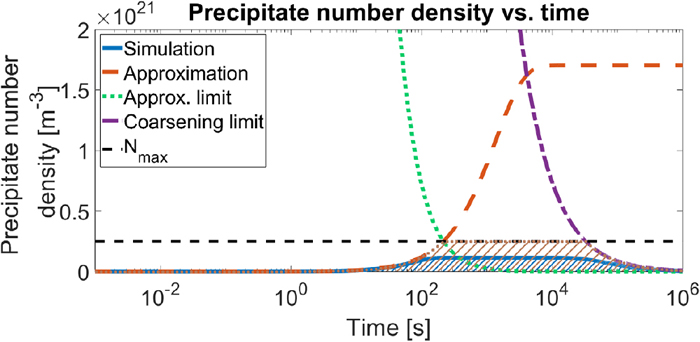
This asymptote is shown in Figs. 1(d) and 1(f). From the asymptotic behaviour a coarsening time can be found at equality in Eq. (25). In other words, when the number density reaches the maximal density N_total, the asymptote from Eq. (25) will intersect the number density at a time t_coarse which can be written as   

$$t_{\text{coarse}}=\frac{\kappa }{N_{\text{total}}},$$(26)

t_coarse is an estimate of the time at which coarsening starts, thus completing the picture of the precipitation development.

2.7. Competition between Nucleation and Growth

In Fig. 1 all potential nucleation sites get occupied at 650°C and 750°C (Figs. 1(b), 1(d)), but not at 850°C (Fig. 1(f)). This is a consequence of a competition between nucleation rate and growth rate. So not all sites will necessarily be used, in particular when the nucleation rate is low compared to the growth rate. When the growth rate is high relative to the nucleation rate, the over-saturation decreases rapidly thus removing the driving force for nucleation before potential nucleation sites had a chance to surpass the critical stage, this can be seen in Fig. 1(f). This means that the fifth restriction listed in section 2.3 is not met.

In section 2.4 for both τ’s it was shown that it is possible to make a quick analysis of the progress of the nucleation and loss of over-saturation, generally it is assumed that the nucleation and decrease in over-saturation are finished after 5 times the characteristic times that were shown (in fact 99.3% of the transition is done). By this reasoning the nucleation is practically finished after 5τ_η, when precipitate growth would not occur. For the start of growth, which was originally defined with t_g,5% as a 5% decrease in over-saturation, one might argue (by virtue of linearising the exponential function) that this decrease in over-saturation occurs after about 0.05τ_λ. Here the end-of-nucleation and start-of-growth have been shifted closer to each other to ensure that they are well separated. Now a dimensionless parameter S may be defined to characterise the condition when all potential nucleation sites will be occupied.   

$$S={log}_{10}\left(\frac{0.05{\tau }_{\lambda }}{5{\tau }_{\eta }}\right)={\text{log}}_{10}\left(\frac{{\tau }_{\lambda }}{{\tau }_{\eta }}\right)-2.$$(27)

When S > 1 the nucleation and growth phases are well separated and the approximations made in sections 2.3 and 2.4 will return good results. In the case that S < 1 not all nucleation sites will be occupied by a precipitate. So N_total is not reached, which means that the approximation needs to be adapted. The maximum reached precipitate number density N_max(< N_total) is estimated to be reached when the over-saturation is removed by the growing precipitates. N_max is estimated from substituting Eq. (11) into Eq. (24):   

$$N\le {\displaystyle \frac{3}{4\pi }}{\displaystyle \frac{C_m^{\text{init}}-C_m^{eq}}{C_m^P}}{\displaystyle \frac{1}{{\left(2D_{\text{eff}}{\displaystyle \frac{C_m^{\text{init}}-C_m^{eq}}{C_m^P-C_m^{eq}}}\right)}^{3/2}{t}^{3/2}}}.$$(28)

Then N_max is found by substituting Eq. (10) and solving the resulting equation for time t:   

$$\begin{array}{l}{N}_{\text{max}}=N_{\text{total}}\left(1-e^{-Z{\beta }^{*}\text{exp}\left(-\mathrm{\Delta }{G}^{*}/\left(k_{B}T\right)\right)t}\right)\\ \hspace{1em}\hspace{1em}\hspace{0.5em}={\displaystyle \frac{3}{4\pi }}{\displaystyle \frac{C_m^{\text{init}}-C_m^{eq}}{C_m^P}}{\displaystyle \frac{1}{{\left(2D_{\text{eff}}{\displaystyle \frac{C_m^{\text{init}}-C_m^{eq}}{C_m^P-C_m^{eq}}}\right)}^{3/2}{t}^{3/2}}}\equiv {\displaystyle \frac{\vartheta }{t^{3/2}}}.\end{array}$$(29)

When N_max is reached nucleation ends, so t may be labelled as a new end-of-nucleation time t_eon. A direct solution can be found from linearising the exponent using Taylor expansion: $t_{\text{eon}}={\left[\vartheta {\tau }_{\eta }/N_{\text{total}}\right]}^{2/5}$, alternatively the bisection method can be used to find N_max. 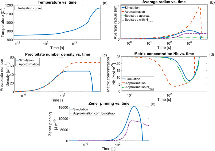This would also return a new coarsening time t′_coarse, with t′_coarse = κ/N_max. This is illustrated in Fig. 3.

Fig. 3.

Here an example is worked out where N_total is not reached. The system is isothermal at 850°C. The solid blue line represents the reference simulation result, the area below is shaded in blue, and the red dashed line the approximation of Eq. (10). The growth asymptote from Eq. (28) is given in the green dotted line, from which N_max is found. And the coarsening asymptote from Eq. (24) is given in the purple dash-dotted line. The maximum number density N_max is also included in the black dashed (horizontal) line. In the brown dotted curve, and the shaded area below, shows the result of the combined approximation results. (Online version in color.)

3. Quasi-isothermal

Temperature is generally not constant in an industrial process. Therefore the isothermal restriction is relaxed, which means that τ_η,Σ, and τ_λ can no longer be assumed time independent. The proposed solution is to create quasi-isothermal time intervals, so the temperature-time curve is approximated by a series of isothermal steps. When the difference in temperature between the steps is small τ_η,Σ, and τ_λ can be updated at the beginning of each domain, the i-th time interval is defined as [t_i, t_i+1]. For each time interval the Eqs. (10), (11), (16) and (19) are connected at the domain boundaries. Before examining the results for a heating and cooling path this is to be re-examined. Consider Eq. (10) rewritten for clarity:   

$$N\left(t\right)=N_{\text{total}}-\left(N_{\text{total}}-N_{\text{pre}}\right)\text{exp}\left(-\frac{t}{{\tau }_{\eta }}\right).$$(30)

On the i-th interval it is rewritten as:   

$$N_i\left(t\right)=N_{\text{total}}-\left(N_{\text{total}}-N_{i-1}\left(t_i\right)\right)\text{exp}\left(-\frac{t-t_i}{{\tau }_{\eta ,i}}\right),$$(31)

At each time interval a boundary condition is needed such that all intervals are linked continuously, this means N_i(t_i) = N_i−1(t_i) at the start of the i-th interval. Where it is noted that N₀(t₀) = N_pre. A similar situation occurs for the growth rate on interval i:   

$$R_i\left(t\right)=\sqrt{2{\mathrm{\Sigma }}_i\left(t-t_i\right)+{\left(R_{i-1}\left(t_i\right)\right)}^2},$$(32)

where R_i(t_i) = R_i−1(t_i), and R₀(t₀) = R^*. And for the concentration on interval i:   

$$C_{m,i}\left(t\right)=\left(C_{m,i-1}\left(t_i\right)-C_m^{eq}\right)\text{exp}\left(-\frac{2}{3}{\left[\frac{\left(t-t_i\right)}{{\tau }_{\lambda ,i}}\right]}^{3/2}\right)+C_m^{eq},$$(33)

where C_m,i(t_i) = C_m,i−1(t_i), and C_m,0(t₀) = $C_m^{\text{init}}$.

The choice for defining the time-interval size is dependent on the cooling or heating rate, because the parameters are temperature dependent. An exact step size for the temperature change is hard to provide, as there are multiple parameters that change at different rates under the influence of temperature. However, it is possible to calculate the parameter values and check the change with each temperature domain, if this change becomes too large a new domain starts. Smaller temperature steps will improve the approximation, however note that common temperatures in heat treatments for steel are higher than > 500°C. Therefore a constant step-size of 1°C could be sufficient, as the change in temperature in each step is much less than 1%, the change in parameter values for each interval is also small. With these quasi-isothermal intervals, and the corrections made in Eqs. (31), (32), and (33) to the approximation, it is possible to approximate the precipitate development for non-isothermal processes. In Fig. 4(a) reheating curve is used, in Fig. 4(d) the dashed line suffers from a computational artefact therefore a jump is seen, the maximum concentration is forced externally as the initial concentration. In Fig. 5 two cooling curves are given, one for the minimum coil temperature, and one for the average temperature.

Fig. 4.

Reheating example, in (a) the temperature-time curve, in (b) the average radius, in (c) the precipitate number density, in (d) the matrix concentration of Nb, and in (e) the calculated Zener pinning pressure. The blue solid lines show the simulation results, the red dashed lines show the approximations from Eqs. (10), (11) and (16). The result of Eq. (19) is also given in (b), and a correction to Eq. (16) is given in (c). (Online version in color.)

Fig. 5.

Similar to Fig. 4, but now for two calculated cooling curves at two different locations in one steel coil. In (a), (c), (e), (g), and (i) respectively the temperature-time curve, the average radius, the precipitate number density, the matrix concentration of Nb, and the calculated Zener pinning pressure at the minimum temperature, and in the same order (b), (d), (f), (h), and (j) for the average temperature. The solid lines show the KWN result, the dashed lines show the approximations. In (j) the difference occurs as in this model only an average radius is considered, whereas in the reference KWN model the precipitate volume fraction is determined from the size distribution. (Online version in color.)

4. Discussion on Validity and Limitations

The approximations are based on a number of assumptions. It is therefore necessary to examine the validity of the assumptions:

1. Isothermal: the most influential parameter is the temperature. Most practical applications are not operating under isothermal conditions. Therefore it was demonstrated that the non-isothermal time-domain can be divided into several isothermal intervals. On each interval the parameters τ_η,Σ, and τ_λ are evaluated, and considered constant on the specific interval.

2. Matrix concentration: the second most important condition is the rate of change in the matrix concentration. This issue is partially resolved by the fact that the approximation is aimed at the initial stage of precipitation, when the concentration is practically constant. After the initial stage the matrix concentration will be changing, but the change can be corrected for in the growth rate to the first order. A correction can be made using the bootstrapping method to find the concentration time-dependence, see Eq. (16). The result can be applied to correct the growth rate, as seen in Eq. (19). Where it must be noted that the approximation does not include coarsening. Another problem that can arise is that the nucleation rate is too low, in that case the original number density limit N_total is not reached before the over-saturation disappears. A new number density limit, N_max, is estimated by using the physical limits on the precipitate population. As this is an estimate based on approximations, the value of N_max is first and foremost an estimate of the order of magnitude of the maximum number density. Still, as it is a great improvement over using N_total, this new limit is applied to further enhance the concentration time-dependence. With these corrections in combination with the LSW theory it is possible to approximate the entire precipitate development cycle, as demonstrated in Figs. 1 and 3.

3. Number of precipitate types and sites: the approximation only counts one type of precipitate, e.g., M_xC_y, and also at one nucleation site. Now if there are multiple precipitate types that do not interfere, i.e., compete for sites or resources they could easily coexist. However competition for, say nitrogen or nucleation sites, is not included. We propose to use this approximation as a simple estimator to predict the precipitation behaviour of the system. One can think of estimating which type of precipitate will appear first or which type will reach the coarsening stage first. This provides key insight into which type of precipitate will dominate the precipitate development of the entire system. It is technically possible to include competition. However this complicates calculations in such a way that the approximate approach loses its appealing feature, which is firstly to provide quick intuitive results.

5. Conclusion

An approximation to the isothermal mean-value precipitation model was derived. First for cases where all available nucleation sites are occupied, the average radius and the number density were approximated. Based on the solutions for average radius and number density an approximation to the time-dependence of the matrix concentration, and from that a correction to the average radius, were found as well. The approximation was then applied under less restrictive conditions, first in the situation where not all sites are occupied before the end of nucleation. Finally the approximation was adapted and applied to non-isothermal situations.

In the derivations the parameters τ_η,Σ, and τ_λ have been defined, where τ_η, and τ_λ are the characteristic times for nucleation and loss of over-saturation respectively (see Eqs. (8) and (15)), and Σ is a characteristic parameter for growth (see Eq. (9)). An intuitive characterisation can be made based on these parameters, for instance when all sites are occupied five times can be defined: (i) a start-of-nucleation time, t_5%; (ii) an end-of-nucleation time, t_95%; (iii) a start-of-growth time t_g,5%; (iv) an end-of-growth time t_g,95%; (v) a coarsening time t_coarse.

Two dimensionless constants were found by taking the quotients of the end and start times: (i) for nucleation t_95%/t_5% = 58.4; (ii) for growth, i.e., when the over-saturation is consumed t_g,95%/t_g,5% = 15.05. Another dimensionless parameter, S = log₁₀(τ_λ/τ_η)−2, was found that characterises the precipitation process as it tells whether the nucleation occurs faster than the growth of the precipitates or not. Secondly it provides an indication to the correctness of the assumption that τ_η,Σ, and τ_λ are time-independent. Parameter S describes the separation of the nucleation and loss of over-saturation during growth. If S > 1, these two events are well separated, but if S < 1 nucleation will not fill all available nucleation sites and growth will occur simultaneously with nucleation. In the S < 1 regime three additional parameters were found: (i) The maximally reached number density, N_max; (ii) the ‘new’ end-of-nucleation time, t_eon; (iii) and an updated coarsening time, t′_coarse.

Together these times and parameters provide an intuitive insight in the precipitate radius and number density development during precipitation before any numerical simulations need to be performed, providing much faster and clear process information. Which is useful for both simulations, and for process control. With this approximation it is possible to get on-line insight in the final product. As demonstrated, the approximation can be applied to a quasi-isothermal approach in which non-isothermal cases can be approximated. The quasi-isothermal approach can be used to approximate results for experimental and industrial precipitate systems.

References

• 1)   T.  Gladman: The Physical Metallurgy of Microalloyed Steels, 2nd ed., CRC Press, Boca Raton, FL, (2001), 176.
• 2)   A.  Deschamps and  Y.  Bréchet: Acta Mater., 47 (1998), 293.
• 3)   A. J.  Ardell: Metall. Trans. A, 16 (1985), 2131.
• 4)   A.  Deschamps,  F.  Livet and  Y.  Bréchet: Acta Mater., 47 (1998), 281.
• 5)   G. E.  Dieter, Jr.: Mechanical Metallurgy, 2nd ed., McGraw-Hill Book Company, New York, NY, (1988), 137.
• 6)   S.  Nandy,  K. K.  Ray and  D.  Das: Mater. Sci. Eng. A, 644 (2015), 413.
• 7)   S.  Esmaeili,  D. J.  Lloyd and  W. J.  Poole: Acta Mater., 51 (2003), 2243.
• 8)   S.  Esmaeili and  D. J.  Lloyd: Acta Mater., 53 (2005), 5257.
• 9)   H. S.  Zurob,  C. R.  Hutchinson,  Y.  Brechet and  G.  Purdy: Acta Mater., 50 (2002), 3075.
• 10)   B.  Dutta,  E. J.  Palmiere and  C. M.  Sellars: Acta Mater., 49 (2001), 785.
• 11)   R.  Kampmann and  R.  Wagner: Decomposition of Alloys: the Early Stages: Proc. 2nd Acta-Scripta Metallurgica Conf., ed. by P. Haasen, V. Gerold, R. Wagner and M. F. Ashby, Pergamon Press, Oxford, UK, (1984), 91.
• 12)   D.  den Ouden,  L.  Zhao,  C.  Vuik,  J.  Sietsma and  F. J.  Vermolen: Comput. Mater. Sci., 79 (2013), 933.
• 13)   M.  Perez,  M.  Dumont and  D.  Acevedo-Reyes: Acta Mater., 56 (2008), 2119.
• 14)   Q.  Du and  Y.  Li: Acta Mater., 71 (2014), 380.
• 15)   Y.  Li,  B.  Holmedal,  H.  Li,  L.  Zhuang,  J.  Zhang and  Q.  Du: Materialia, 4 (2018), 431.
• 16)   J. D.  Robson: J. Nucl. Mater., 476 (2016), 123.
• 17)   H. M.  Hulburt and  S.  Katz: Chem. Eng. Sci., 19 (1964), 555.
• 18)   M.  Volmer and  A.  Weber: Z. Phys. Chem., 119U (1926), 277 (in German).
• 19)   Ya. B.  Zeldovich: Acta Physicochim. USSR, 18 (1943), 1.
• 20)   R.  Becker and  W.  Döring: Ann. Phys., 416 (1935), 719 (in German).
• 21)   J. D.  Robson: Acta Mater., 52 (2004), 4669.
• 22)   C.  Zener: J. Appl. Phys., 20 (1949), 950.
• 23)   R.  Gómez-Ramírez and  G. M.  Pound: Metall. Trans., 4 (1973), 1563.
• 24)   S.  Okaguchi and  T.  Hashimoto: ISIJ Int., 32 (1992), 283.
• 25)   K.  Narita: Trans. Iron Steel Inst. Jpn., 15 (1975), 145.
• 26)   I. M.  Lifshitz and  V. V.  Slyozov: J. Phys. Chem. Solids, 19 (1961), 35.
• 27)   C.  Wagner: Z. Elektrochem., 65 (1961), 581 (in German).
• 28)   J. J.  Hoyt: Acta Metall. Mater., 39 (1991), 2091.
• 29)   M. V.  Speight: Acta Metall., 16 (1968), 133.
• 30)   H.  Kreye: Z. Metallkd., 61 (1970), 108.
• 31)   A. F.  Smith: J. Less-Common Met., 9 (1965), 233.
• 32)   A. F.  Smith: Acta Metall., 15 (1967), 1867.