Modeling of Wall Shear Stress Induced Inclusion Transport and Removal in Multi-Strand Tundish

Abstract

Erosion of refractory lining due to flow induced wall shear stress is one among severe problems that shop floor personnel face in continuous casting tundish operation. It decreases the lining life and increases overall operational cost. Wall shear stress due to turbulent flow is one of the major factors of erosion of lining in tundish. Inclusion generation due to erosion creates surface defects that may lead to the rejection of the final products. Turbulent inhibitor box (TIB) helps in reducing the wall shear stress by confining the turbulent flow zone and hence changes the flow pattern. In the present work, three-dimensional fluid flow study has been carried out to investigate the flow induced wall shear stress. High shear stress zones (HSSZ) are taken as potential inclusion generation sites. Different sizes of inclusions are injected from those sites and their paths are tracked. It is found that the shape of TIB significantly affects the flow induced wall shear stress and inclusion removal rate. Results indicate that tundish with TIB 3 arrangement exhibited minimum wall shear stress at all walls. TIB 2 coupled tundish gives the highest removal rate in case of bottom wall originated small size inclusions (<= 80 µm) and least removal rate in case of curve wall originated inclusions.

1. Introduction

Design of tundish has always been an area of prime concern for steelmakers and hence in stage of continuous development. In the initial stage, it acted as a reservoir and later evolved into a useful reactor for liquid steel cleanliness. Apart from distributor and buffer, it plays a key role towards quality of the casting obtained by solidification of liquid steel in the copper mold . Due to the growing demand for quality steel casting, tundish relevance is increasing in a continuous casting operation. Modern day tundish helps in various metallurgical operations such as homogenization of steel temperature, inclusion removal, superheat control, flow control, superheat control, wall erosion reduction and decrease dead volume. Different types of refractories grades are used in lining of tundish walls, dams and weirs, impact pads, flow control devices, tundish nozzles, etc. Refractory lining design and its quality have a significant influence on the operational parameters of tundish such as superheat requirement, speed of machine, nozzle clogging, etc. Due to high temperature involved, refractory lining are to be designed to withstand thermal shock, prevent thermal loss and resist corrosion and erosion. Lining material erodes due to mechanical wear, thermal shock, turbulent fluid flow, slag attack, etc. Figure 1 present all possible causes of erosion of refractory lining.

Fig. 1.

Possible causes of erosion of refractory lining in tundish.

Inclusions due to lining erosion are one of the major sources of impurity in continuous casting (CC) tundish and give rise to surface defects that may sometime lead to final product rejection. Mechanical erosion of refractory lining occurs due to high flow induced shear stress. High turbulence regions of tundish are prone to high shear stress. For clean and sound casting, relining of tundish is very crucial after a certain number of casting. Cost associated with relining is a significant contributor to the overall operation cost in CC operation. Therefore, the life cycle of lining is an issue of concern for steelmakers. Among all the factors shown in Fig. 1, turbulent fluid flow is a significant factor that affect the wear of lining. Turbulent fluid flow assists the incursion of iron oxide into the refractory lining. Interaction of fluid flow with tundish wall results in flow induced wall shear stress and consequently erodes the refractory lining. Hydrodynamic of fluid plays an important role in determining the extent of fluid induced shear stress. Turbulent intensity of fluid is determined by turbulent kinetic energy, one of the turbulence parameter. Flow control devices such as weir, dam and turbulent inhibitor box (TIB) minimize the turbulence parameters in tundish , hence helps in reducing wall shear stresses and in guiding the fluid to outlet smoothly. Shape of TIB plays major role in suppressing the eddy motion due to turbulence, decreasing turbulence flow affected area and also affects the flow characteristics. So good knowledge of the effect of shape of TIB on flow behaviour and subsequently induced wall shear stress on tundish wall is useful for steel makers to decide the optimum shape of TIB. Most of the researches focus their study on the interaction between fluid flow, inclusion, slag and argon flow using physical and mathematical modeling.^{1,2,3,4,5,6,7,8,9,10)} Few works of literature deal with fluid flow interaction with tundish walls. Effect of tundish design parameters such as wall angle, curvature radius with flow control devices integrated tundish on flow induced stress have been studied. Singh et al.¹¹⁾ Numerical study of the effect of tundish shapes on wall shear stress has been carried out. Siddhiqi and Jha.¹²⁾ Many studies are reported on the effect of TIB configurations on flow characteristics.^{13,14,15,16,17,18,19)}

All available works of literature on inclusion transport and removal are based on their origin from the ladle. Inclusion that originates from ladle due to deoxidation products, ladle lining erosion and come to tundish via nozzle were considered in previous studies.^{20,21,22,23,24,25,26,27)} However, there are multiple sites of inclusions generation in tundish due to refractory lining erosion. Slag entrainment due to turbulence flow and deoxidation products of ladle are another source of inclusion generation. Study of the behaviour of slag interaction with fluid has been reported by Siddhiqi and Jha.^28,29) All inclusion generation sites are reported in literature. Sinha and Sahai.²¹⁾

Tundish refractory lining erosion due to flow induced wall shear stress is another major source of inclusion generation. So far, very few of literature is available on the transport and removal behaviour of inclusions generated in high shear stress zones (HSSZ). Therefore, it has been intended to study inclusion generation and their transport due to lining erosion caused by flow induced shear stress for tundish with and without the use of TIB. The focus of the present study is to investigate the effect of different TIB configurations on wall shear stress due to turbulent flow and to study transport of inclusions generated due to refractory lining erosion of tundish walls.

2. Physical Description of the Problem

The geometric details of industrial multi strand tundish without TIB and with use of TIB in the present study are shown in Fig. 2(a). Half of tundish is shown due to symmetry about inlet plane and the diameter of the shroud and all outlets are shown as 70 mm and 20 mm respectively. Geometry details of three different TIB are shown in Figs. 3(a)–3(c). Shape of TIB 1 is simple, TIB 2 has an outward draft on the inner and outer wall whereas TIB 3 has an inward draft with little closing on top.

Fig. 2.

a) Geometric details of bare tundish, b) Tundish with TIB.

Fig. 3.

Geometric details of a) TIB 1, b) TIB 2, c) TIB 3. (Online version in color.)

3. Mathematical Model Description

The academic research CFD software FLUENT 19.2 is used for solving governing differential equations. Following assumptions are made:-

a) Molten steel flow is assumed to be incompressible Newtonian steady state flow.

b) Tundish is operated under isothermal conditions.

c) Gas entrapment is neglected.

d) Top surface of tundish is considered flat with insignificant slag depth.

e) Shape of inclusion particles is assumed to be spherical.

3.1. Fluid Flow Model

For flow field calculations, three dimensional continuity and Navier-stokes equations are solved for incompressible Newtonian fluids. These steady state equations can be expressed by Eqs. (1)–(2).

Continuity   

$$\frac{\partial (\rho u_i)}{\partial x_i}=0$$(1)

Momentum   

$$\frac{\partial (\rho u_i{u}_j)}{\partial x_j}=\frac{\partial }{\partial x_j}\left[{\mu }_e\left(\frac{\partial u_i}{\partial x_j}+\frac{\partial u_j}{\partial x_i}\right)\right]-\frac{\partial p}{\partial x_i}+\rho \overrightarrow{g}$$(2)

Where   

$${\mu }_e=\mu +{\mu }_t$$

  

$${\mu }_t=C_4\rho \frac{k^2}{\epsilon }$$

In the present work, k–ε realizable turbulence model is used. The governing equations for turbulent kinetic energy and its rate of dissipation are given by Eqs. (3)–(4).^30,31,32)   

$$\frac{\partial }{\partial x_j}(\rho k{u}_j)=\frac{\partial }{\partial x_j}\left[\left(\mu +\frac{{\mu }_t}{{\sigma }_k}\right)\frac{\partial k}{\partial x_j}\right]+G_k-\rho \epsilon$$(3)

  

$$\frac{\partial }{\partial x_j}(\rho \epsilon u_j)=\frac{\partial }{\partial x_j}\left[\left(\mu +\frac{{\mu }_t}{{\sigma }_{\epsilon }}\right)\frac{\partial \epsilon }{\partial x_j}\right]+\rho C_{1}S\epsilon -\rho C_2\frac{{\epsilon }^2}{k+\sqrt{v\epsilon }}$$(4)

Where   

$$G_k={\mu }_t\frac{\partial u_j}{\partial x_i}\left(\frac{\partial u_i}{\partial x_j}+\frac{\partial u_j}{\partial x_i}\right)$$(5)

  

$$C_1=max.\left[0.43,\mathrm{\hspace{0.17em} }\frac{\eta }{\eta +5}\right],\mathrm{\hspace{0.17em} }\mathrm{\hspace{0.17em} }\mathrm{\hspace{0.17em} }\eta =S\frac{k}{\epsilon },\mathrm{\hspace{0.17em} }\mathrm{\hspace{0.17em} }\mathrm{\hspace{0.17em} }S=\sqrt{2S_{ij}{S}_{ij}}$$

  

$$C_{\mu }=\frac{1}{A_O+A_S\frac{k{U}^{*}}{\epsilon }}\mathrm{\hspace{0.17em} },\mathrm{\hspace{0.17em} }\mathrm{\hspace{0.17em} }\mathrm{\hspace{0.17em} }\mathrm{\hspace{0.17em} }\mathrm{\hspace{0.17em} }\mathrm{\hspace{0.17em} }\mathrm{\hspace{0.17em} }{U}^{*}=\sqrt{S_{ij}{S}_{ij}+{\hat{\mathrm{\Omega }}}_{ij}{\hat{\mathrm{\Omega }}}_{ij}}$$

${\overline{\mathrm{\Omega }}}_{ij}$ is the mean rate of rotation tensor viewed in a rotating reference frame with the angular velocity ω_k. The model constants A_O and A_s are given by   

$$A_O=4.04,\mathrm{\hspace{0.17em} }\mathrm{\hspace{0.17em} }{A}_s=\sqrt{6}\mathrm{\hspace{0.17em} }cos\varnothing$$

  

$$\begin{array}{l}\varnothing =\frac{1}{3}{cos}^{-1}\sqrt{6}W,\mathrm{\hspace{0.17em} }W=\frac{S_{ij}{S}_{jk}{S}_{ki}}{{\hat{S}}^3},\mathrm{\hspace{0.17em} }\hat{S}=\sqrt{S_{ij}{S}_{ij}},\mathrm{\hspace{0.17em} }\\ S_{ij}=\frac{1}{2}\left(\frac{\partial u_j}{\partial x_i}+\frac{\partial u_i}{\partial x_j}\right)\end{array}$$

Wall shear stress is computed using the following equation.¹¹⁾   

$$\begin{array}{l}{\displaystyle \frac{\rho v_p{c}_3^{\raisebox{1ex}{$1$}\!\left/ \!\raisebox{-1ex}{$4$}\right.}{k}_p^{\raisebox{1ex}{$1$}\!\left/ \!\raisebox{-1ex}{$2$}\right.}}{{\tau }_w}}={\displaystyle \frac{1}{k}}\text{ln}\left(E{\displaystyle \frac{\rho y_p{C}_3^{\raisebox{1ex}{$1$}\!\left/ \!\raisebox{-1ex}{$4$}\right.}{k}_p^{\raisebox{1ex}{$1$}\!\left/ \!\raisebox{-1ex}{$2$}\right.}}{\mu }}\right)\\ C_3=0.09,\mathrm{\hspace{0.17em} }\mathrm{\hspace{0.17em} }E=9.793\end{array}$$(6)

3.2. Inclusion Modeling

Inclusions particles trajectories are calculated using langrangian particle tracking method. Particle mean velocity is obtained using force balance equation which includes drag and buoyancy force as given by Eq. (7).^13,24)   

$$\frac{d{u}_p}{dt}=F_D(u-u_p)+\frac{g({\rho }_p-\rho )}{{\rho }_p}+F_x$$(7)

Where F_D(u−u_p) is drag force per unit mass of particles.   

$$F_D=\frac{18\mu }{{\rho }_p{d}_p^2}\frac{C_D{R}_e}{24},\mathrm{\hspace{0.17em} }\mathrm{\hspace{0.17em} }\mathrm{\hspace{0.17em} }\mathrm{\hspace{0.17em} }\mathrm{\hspace{0.17em} }{R}_e=\frac{\rho d_p\left|u_p-u\right|}{\mu }$$

To simulate the chaotic effect of the turbulent eddies on the particle paths, a discrete random walk model is applied during inclusion trajectory calculations in which a random velocity vector $u_p^{\prime }$ is added to the calculated time-averaged vector, ${\overline{u}}_p$ to obtain the inclusion velocity u_p at each time step as it travels through the fluid. Each random component of the inclusion velocity is proportional to the local turbulent kinetic energy level, k according to the following equation.¹³⁾   

$$u_p^{\prime }={\zeta }_i\sqrt{\overline{u_i^{\prime }{}^2}}={\zeta }_i\sqrt{\frac{2k}{3}}$$(8)

Where ζ_i is a random number, normally distributed between −1 and 1 that changes at each time step. Inclusions are injected computationally at many different locations distributed homogeneously over the inlet plane. Each trajectory is calculated through the constant steel flow field until the inclusion either is trapped or exits the tundish outlet.

3.3. Operating and Boundary Conditions

At the planes of symmetry, the normal gradient of tangential velocity and the normal velocity components are set to zero. The walls are set to a no slip condition. Zero shear stress boundary condition provided to the top surface. Velocity at inlet is mentioned in Table 2 is set at inlet. The inlet turbulent kinetic energy k_in and energy dissipation rate ε are evaluated using Eqs. (9)–(10)²⁷⁾ as shown below. Zero relative pressure is set at all outlet cell surfaces.   

$$k_{in}=0.01u_{in}^2$$(9)

  

$${\epsilon }_{in}=\frac{k_{in}^{\raisebox{1ex}{$3$}\!\left/ \!\raisebox{-1ex}{$2$}\right.}}{R_{Nozzle}}$$(10)

Table 2. Material properties and operating parameters.

Parameter	Value
Molten steel viscosity	0.0068 kg ms−1
Molten steel density	7400 kg m−3
Inlet velocity	1.2 m s−1

For inclusion transport modeling, inclusions are assumed to be trapped once reaching top surface and those touching side and bottom walls are considered to reflect. Inclusions reaching outlets are assumed to be escape. Density of inclusion to liquid steel is 0.56.

3.4. Numerical Solution Procedure

Three-dimensional structured hexagonal mesh is used for numerical simulations. Turbulent kinetic energy values are computed on different walls of bare tundish for grid independence study. Numerical computation is carried out by using three different numbers of grid elements i.e. very fine grid (1.8 million elements), fine grid (1.4 million elements) and coarse grid (1.1 million elements). Maximum turbulent kinetic energy values are given in Table 3. There is a small change in wall shear stress values on changing grid elements from coarse to fine, but negligible change is observed on fine to very fine grid. Hence, the fine grid as base grid size is used for further study.

Table 3. Maximum turbulent kinetic energy values at different wall for different grid sizes of bare tundish.

Max. Turbulent Kinetic Energy (m2/s2) Grid elements (m)	Bottom wall	Front wall	Curve wall
Coarse grid (1.1 m)	0.027	0.00029	0.00195
Fine grid (1.4 m)	0.03	0.00024	0.00205
Very fine grid (1.8 m)	0.03	0.00025	0.00204

The numerical modeling starts with discretization of set of governing partial differential Eqs. (1), (2), (3), (4) for determination of steady state flow field using CFD software Fluent R19.2. To obtained the initial solution, transport equations are discretized by second order upwind scheme. In the numerical solution scheme, Semi Implicit Method for Pressure Linked Equation (SIMPLE) algorithm is used for pressure velocity coupling in the momentum equation and the body force weighted pressure approach for the spatial discretization due to gravity is considered. A realizable k-ε turbulence model is employed to simulate the turbulence and first order scheme is used for the same. Flow induced shear stress is computed at tundish walls for all cases as given in Table 1.

Table 1. Simulations cases.

S. No.	Cases	Description
1	C1	Bare Tundish
2	C2	Bare Tundish with TIB 1
3	C3	Bare Tundish with TIB 2
4	C4	Bare Tundish with TIB 3

Once the steady state flow field is determined, Inclusions transport Eq. (7) is solved for each inclusion as it traveled in the established flow field. In this study, inclusions originated from tundish walls due to lining erosion caused by flow induced shear stress are considered. Therefore, HSSZ on tundish walls were identified and positions of corresponding nodes in terms of their coordinates are computed. After lining erosion, initial transport of inclusion is mainly governed by the nearby turbulent zone flow field. Therefore, flow velocity components of nearby turbulent flow field nodes are calculated. Inclusions are injected from HSSZ nodes with velocity components of corresponding turbulent field nodes and their paths are tracked.

4. Validation Study

The present work is validated with a previously published result. Ruckert et al.³³⁾ of water model for a single strand tundish case. In the published study, particles were injected from the inlet and tracked in previous calculated flow field. Inclusions touching sidewalls and top surface were assumed to reflect and trapped boundary conditions respectively. Escape condition was assigned to outlet. It can be seen from Fig. 4 that there is satisfactory matching between removal rate (Eq. (11)) curves. Therefore, the current numerical model is appropriate for further study.   

$$\mathrm{R}\mathrm{e}\mathrm{m}\mathrm{o}\mathrm{v}\mathrm{a}\mathrm{l}\mathrm{\hspace{0.17em} }\mathrm{r}\mathrm{a}\mathrm{t}\mathrm{e}(\%)=\frac{N_{in}-N_{out}}{N_{in}}x100$$(11)

Fig. 4.

Vailidation study.

5. Results and Discussions

5.1. Wall Shear Stress for Different Cases

The simulations are carried out for all the cases, as given in Table 1. The contours of wall shear stress on tundish walls and velocity vector profiles are shown for each case. Effect of TIB geometry on wall shear stress are studied. Curve profile wall named as a curve wall, and the wall opposite to curved wall is named as front wall.

5.1.1. Bare Tundish (C1)

Velocity vectors at the vertical symmetry plane is shown in Fig. 5(d). Fluid comes from the inlet and divides into two streams after striking on bottom wall and goes upwards. Left side streams form left circular loop and responsible for second peak wall shear stress region on curve wall as shown in Fig. 5(b). Similarly, the right stream form another circular loop and accountable for high shear stress on the front wall as shown in Fig. 5(c). Velocity vector at the vertical outlet plane is shown in Fig. 5(e). Velocity vectors are very dense near the left edge of plane and mid region of outlet 1 and outlet 2 and contribute in HSSZ on curve wall. Spread of peak wall shear stress region at curve wall and front wall is in x direction, which can be understood by negative x direction of velocity vectors as in Fig. 5(e). Contour of wall shear stress of bottom wall is shown in Fig. 5(a). After striking bottom wall, streams move symmetrically with high velocity in opposite direction and give rise to high and symmetrically distributed wall shear stress (Fig. 6(b)). Maximum wall shear stress at bottom wall is 21 Pa, which is high near to impact point and then decreases gradually. Maximum shear stress values at curve wall and front wall are 3.1 Pa and 0.432 Pa, which is very less compared to bottom wall. Hence, erosion will more at bottom wall compare to other walls. Therefore, TIB coupled tundish is advisable and practice by many steelmakers now a days and used in further study. Figure 6 shows the variation of wall shear stress and velocity along polyline at curve wall and bottom wall. Polyline is generated in the HSSZ adjacent turbulent region and it has a constant height from tundish bottom (equal to z coordinate of highest shear stress node). Velocity values at nearby turbulent zone nodes are calculated and plotted on the same figure. It can be seen that wall shear stress and velocity vary in a similar fashion. Positions of peak and trough of wall shear stress and velocity curves almost similar. Therefore high shear stress regions are also high turbulent kinetic energy regions. Double peaks in case of bottom wall curve are due to molten metal from inlet strikes at bottom wall and divided into two streams, which leads to the formation of two circulation zones. Therefore, value of wall shear stress varies proportionally with velocity.

Fig. 5.

Bare tundish (C1): Wall shear stress contours of a) Bottom wall, b) Curve wall, c) Front wall, Velocity vectors at d) Symmetry plane, e) Outlet plane. (Online version in color.)

Fig. 6.

Bare tundish (C1): Variation of wall shear stress on HSSZ and velocity along polyline lie in the turbulent region adjacent to HSSZ at a) Curve wall, b) Bottom wall.

5.1.2. Bare Tundish Coupled with TIB 1 (C2)

Flow behaviour changes on integrating TIB with bare tundish. After striking fluid to TIB, divide into two equal streams (Fig. 7(d)). Fluid in the top left side forms a circular loop and contributes to high shear stress at left edge of curve wall (Fig. 7(b)) and responsible for second peak in wall shear stress curve as shown in Fig. 8(b). Turbulent kinetic energy in this region is very high (Fig. 8(a)). Fluid from inlet, after striking at the tundish bottom, directed towards the curve wall with high speed, which results in high shear stress and therefore, HSSZ on the curve wall shifts towards the right (Fig. 8(a)) compared to C1. Due to the higher level of TIB bottom wall, the peak wall shear stress is high compared to C1 (Fig. 8(b)). So, the addition of TIB shift the wall shear affected zone. Velocity vectors are very dense at the top left of symmetry plane. Outlet plane velocity vectors are shown in Fig. 7(e). It can be seen density of vectors is very high at the top of outlet 1 and forms the circulation zone. High velocity near this zone results in high shear stress at the top left of front wall as shown in Fig. 7(c). The distribution of peak wall shear stress at the front wall is in z direction, which can understood by z direction velocity vectors at the top side, as shown in Fig. 7(e). Wall shear stress contour of bottom wall is shown in Fig. 7(a). Distribution of shear stress is symmetric about the inlet axis because the stream divides symmetrically after striking at the bottom wall of TIB and can be confirmed with double equal peaks of the curve as shown in Fig. 8(b). Maximum shear stress is 22.4 Pa, which is more compared to previous case C1 because level of TIB bottom wall little up than the tundish bottom wall, which leads to less dissipation of turbulent kinetic energy. Maximum wall shear stress at the curve wall and front wall are 0.76 Pa and 0.1 Pa respectively, which are less corresponding to previous case C1. Therefore, TIB decreases wall shear stress significantly by minimizing the turbulence flow and confining the turbulent flow. Although bottom wall shear stress is high, but shear stress affected zone confined to in less area. So TIB helps in decreasing the wall shear stress, which results in less erosion and leads to a higher life of tundish lining.

Fig. 7.

Bare tundish with TIB 1 (C2): Wall shear stress contours of a) Bottom wall, b) Curve wall, c) Front wall, Velocity vectors at d) Symmetry plane, e) Outlet plane. (Online version in color.)

Fig. 8.

Bare tundish with TIB 1 (C2): Variation of wall shear stress on HSSZ and velocity along polyline lie in the turbulent region adjacent to HSSZ at a) Curve wall, b) Bottom wall.

5.1.3. Bare Tundish Coupled with TIB 2 (C3)

In this case, outward draft is provided to TIB walls. Velocity vectors at the symmetry plane are almost same as in previous case C2, except there is no bottom to top flow at the left side of the inlet (Fig. 10(d)). Due to TIB walls outward draft, there will be more free flow after striking on TIB bottom wall. So, the spread of the shear stress zone affected area will be more, which can be seen in Figs. 10(b) and 10(c). Location of HSSZ on the curve wall is almost same as of C2, as shown in Fig. 9(a). The magnitude of velocity near the peak wall shear stress region is same as in previous case C2 (Fig. 9(a)). Vectors are very dense at the left and right side of the inlet and give rise to high shear stress on the curve wall and front wall near to edges. Figure 10(e) represents the velocity vector at the outlet plane. Fluid comes from both sides in outlet 1, from backward in outlet 2 and from forward in outlet 3. Circular loop forms at mid region of outlet 1 and outlet 2. The spread and magnitude of loop at the top of outlet 1 are high compared to previous case C2 and gives rise to high shear stress on the front wall (Fig. 10(c)). Shear stress affected zone is more but maximum shear stress value is 0.52 Pa, which is less compared to previous cases. Figure 10(a) represents contours of bottom wall shear stress. Fluid stream from inlet is divided equally after striking at the tundish bottom and therefore, shear stress and velocity distribute symmetrically about inlet axis as shown in Fig. 9(b). Due to outward draft of TIB walls, peak wall shear stress region shifts further away from inlet compared to C2 case. Maximum shear stress is 24.8 Pa, which is little higher than the previous case. This is due to higher maximum velocity. So draft on TIB walls makes little difference in comparison in terms of reducing the wall shear stress.

Fig. 9.

Bare tundish with TIB 2 (C3): Variation of wall shear stress on HSSZ and velocity along polyline lie in the turbulent region adjacent to HSSZ at a) Curve wall, b) Bottom wall.

Fig. 10.

Bare tundish with TIB 2 (C3): Wall shear stress contours of a) Bottom wall, b) Curve wall, c) Front wall, Velocity vectors at d) Symmetry plane, e) Outlet plane. (Online version in color.)

5.1.4. Bare Tundish Coupled with TIB 3 (C4)

Inward draft on walls with little closing at the top is provided to TIB. After striking to TIB bottom stream divided symmetrically. Inward draft helps in guiding flow to upward direction as shown in Fig. 11(d). A small loop forms at the left side of the inlet and gives rise to higher shear stress near the edge of the curve wall as shown in Fig. 11(b). Although the size and intensity of loop are less compared to previous cases C2 & C3 therefore, shear stress is less compared to these cases. Location of HSSZ is further shifted upward. Top closing helps in minimizing the turbulence. Velocity nearby HSSZ zone on both curve and front walls is significantly less compared to previous cases(Figs. 12(a) and 12(b)), which in turn decreases turbulent kinetic energy. Therefore HSSZ wall shear stress is less. Density of vectors is very high adjacent to the inlet. Big circulation loop forms right side of the inlet and contributes to high shear stress at the front wall (Fig. 11(c)). Highly dense and upward direction velocity vectors at the left side of the inlet give rise to high shear stress adjacent to the left edge of the curve wall as shown in Fig. 11(b). Velocity vectors at outlet plane are shown in Fig. 11(e). Spread of the peak shear stress region at curve wall and front wall are in x direction, which can be understood by x direction velocity vectors as shown in Fig. 11(e). Contour of bottom wall shear stress is shown in Fig. 11(a). Shear stress distributes symmetrically about inlet axis. Maximum shear stress is 19.9 Pa, which is less compared to previous cases (C1, C2 and C3). This is due to the fact that there is no full circulation loop in TIB. Therefore turbulent kinetic energy is also less (Fig. 12(b)). Maximum values of shear stress at the front wall and curve wall are 0.115 Pa and 0.23 Pa respectively. So peak shear stress values at all walls are less compare to other previous cases (C1, C2 and C3). Therefore, erosion will be less and life of tundish lining will be more.

Fig. 11.

Bare tundish with TIB 3 (C4): Wall shear stress contours of a) Bottom wall, b) Curve wall, c) Front wall, Velocity vectors at d) Symmetry plane, e) Outlet plane. (Online version in color.)

Fig. 12.

Bare tundish with TIB 3 (C4): Variation of wall shear stress and velocity along polyline line in the region of HSSZ at a) Curve wall, b) Bottom wall.

5.2. Inclusion Transport Modeling

Inclusion generation due to erosion of refractory lining caused by flow induced shear stress has been predicted. Due to the very low magnitude of shear stress on the longitudinal wall as compared to other walls, it is not taken into consideration for inclusion generation. Results are presented in two parts: In the first part, results of the transport behavior of bottom wall generated inclusions are shown and in the second part, curve wall results are presented. Comparative analysis of inclusion diameters of 20 μm and 160 μm are presented for each case. Four particles are tracked and their behavior is studied.

5.2.1. Inclusion Transport (Bottom Wall)

Typical trajectories of 20 μm and 160 μm particles injected from bottom HSSZ are shown in Figs. 13 and 14 respectively. Only four particle trajectories are displayed in different colors for each case. For analyzing particle transport and removal and further to analyze the path of inclusions, pathlines of flow are shown in Fig. 15. Pathlines are more uniformly random distributed and covers full length in case of bare tundish (Fig. 15(a)). Due to the formation of circular loops, particles are trapped in that zone. Trajectory of 20 μm follows similar paths before getting trapped or escape (Fig. 13(a)). Only one particle gets trapped out of four. In cases C2-C4, TIB directs pathlines towards outlets (Figs. 15(a)–15(d)). This effect is more pronounced in case C4. Hence, it can be inferred that TIB significantly affects flow direction and drifts the flow towards outlets. The effect of such flow can be observed on the transport of small particles, which also tend to move towards outlets (Figs. 13(b)–13(d)).

Fig. 13.

Trajectory of 20 μm particles injected from bottom surface for cases a) C1, b) C2, c) C3, d) C4. (Online version in color.)

Fig. 14.

Trajectory of 160 μm particles injected from the bottom surface for cases a) C1, b) C2, c) C3, d) C4. (Online version in color.)

Fig. 15.

Pathlines of a) C1, b) C2, c) C3, d) C4. (Online version in color.)

Trajectories of 160 μm particles are shown in Fig. 14. In case of bare tundish, particles move randomly near inlet region before being trapped at slag metal interface or escape from outlets (Fig. 14(a)). This phenomena is not observed in TIB coupled tundishes (Figs. 14(b)–14(d)). Rather, the particles directly move towards the top surface. Due to hindrance created by TIB, movement of particles lead to the formation of loops in TIB before escaping from that region. Buoyancy force dominates over drag force in case of large particles, hence large size particles are more prone to float at slag metal interface and have lesser tendency to move towards the mold region. Reverse effect is observed in case of small particle size particles, where the motion of particles are governed by the molten metal flow.

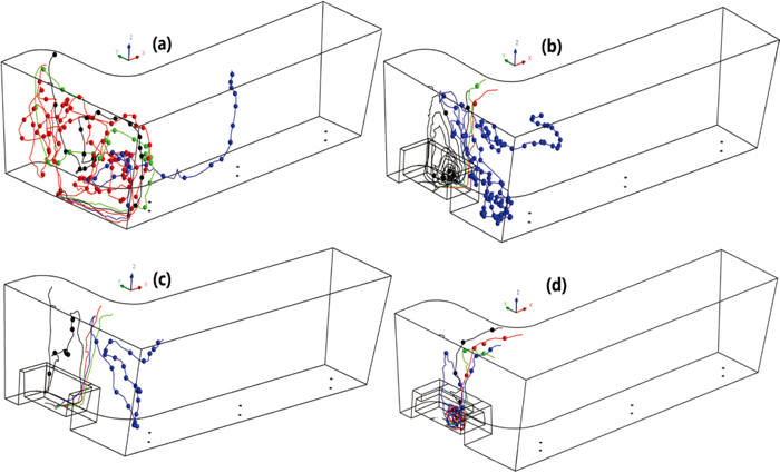
5.2.2. Inclusion Transport (Curve Wall)

Transport behavior of 20 μm and 160 μm inclusions are shown in Figs. 16 and 17 respectively. Initial movement can be explained by velocity vectors of the surface which is offset to curve wall and lie in the nearby turbulent region, as shown in Fig. 18. Small green contour indicates the inclusion injection site corresponding to HSSZ on the curve wall. Velocity vectors are in upward direction close to HSSZ in the case of bare tundish (Fig. 18(a)), which drift inclusions in same direction (Figs. 16(a) and 17(a)). Circular loop form by 20 μm inclusions is due to similar path follow by pathlines (Fig. 15(a)). Direction of velocity vectors is downward near to HSSZ region in case of TIB coupled tundishes (Figs. 18(b)–18(d)). After impact at TIB bottom face, short circuit is formed and flow is directed towards the curve wall. However, due to the hindrance created by the wall, it moves in downward direction and drifts inclusions also in the same way (Figs. 16(b)–16(d) and Figs. 17(b)–17(d)). Velocity vectors are separated in two opposite directions at HSSZ. Left side vectors form a loop and right side vectors go into the outlets region (Fig. 18(b)). Therefore, red and green color inclusions are mostly confined to the left region of TIB and others are moved in outlets region (Figs. 16(b) and 17(b)). However, in case of 160 μm, all the particles are transported towards the top surface due to increase dominance of buoyancy force and hence get trapped (Fig. 17(b)). Direction of velocity vectors are right to the HSSZ (Fig. 18(c)), hence inclusion transport is also in the same direction (Figs. 16(c) and 17(c)) and 160 μm move towards the upper region and subsequently trapped at the top surface (Fig. 17(c)). Pathlines are specifically directed to outlets after impact at the TIB bottom surface (Fig. 15(a)). Therefore 20 μm inclusions first drift to the right of HSSZ and than after impact at the bottom wall, is directed to different outlets (Fig. 16(d)). 160 μm particles follow a similar path initially, but due to high buoyancy, it gets trapped to the top surface (Fig. 17(d)).

Fig. 16.

20 μm particles trajectory injected from curve wall a) C1, b) C2, c) C3, d) C4. (Online version in color.)

Fig. 17.

160 μm particles trajectory injected from curve wall a) C1, b) C2, c) C3, d) C4. (Online version in color.)

Fig. 18.

Velocity vectors at surface offset from curve face lie in the nearby turbulent region a) C1, b) C2, c) C3, d) C4.

5.2.3. Inclusion Removal Rate

Overall removal rate of inclusion generated from the bottom wall and curve wall is shown in Figs. 19 and 20 respectively. 120 particles were injected from HSSZ nodes of bottom wall and curve wall. Removal rate is calculated using Eq. (11). It can be seen that bigger particles have high removal rate for all cases due to the high buoyancy force. Small size inclusions removal rate is high in the case of TIB coupled tundish compared to bare tundish in the case of bottom wall originated inclusions (Fig. 19). Tundish C3 is found to best for small size inclusion removal rate (<= 80 μm). Coupling of TIB and its shape does not affect the inclusion removal rate for inclusion size greater than 100 μm (Fig. 19). Inclusions originated from Curve wall HSSZ have less removal rate in the case of TIB integrated tundish as compared to that from base tundish (Fig. 20). Therefore, integration of TIB is found to deleterious in this case.

Fig. 19.

Removal rate of inclusion generated from bottom wall.

Fig. 20.

Removal rate of inclusion generated from curve wall.

6. Conclusions

Flow-induced wall shear stress has been analyzed for various designs of TIB coupled tundish using three dimensional numerical simulation approach. Based on the wall shear stress values, refractory lining erosion sites are identified. Inclusion are injected from these sites and their transport behavior is analyzed. Shape of TIB significantly affects the flow induced wall shear stress and inclusion removal rate. The following conclusions can be drawn out from the investigations.

(1) The TIB coupled tundishes contribute significantly towards reducing the flow-induced shear stress on the walls. Therefore, it helps in increasing the life of the refractory lining.

(2) TIB helps in decreasing the flow induced shear stress affected area at the bottom wall.

(3) Shear stress is maximum for bottom wall, therefore bottom wall is more prone to lining erosion as compared to other walls.

(4) Tundish with TIB (Case-C4) has proven to be the best configuration among all cases in terms of reduction in the shear stress values.

(5) Bottom wall originated big sized inclusion (>= 100 μm) removal rate is unaffected by TIB shape and comes out almost equal to the bare tundish. Tundish C3 gives the highest removal rate for small size (<= 80 μm).

(6) In the case of curve wall originated inclusions, the removal rate is found to be least in case of tundish C3 and highest for bare tundish C1.

Nomenclatures

u: Molten steel velocity (m/s)

x_i: Cartesian Coordinate direction along x, y & z

ρ: Density (kg m⁻³)

t: Time (second)

g: Gravitational acceleration (9.81 m/s²)

C₁, C₂, C_μ: Turbulent constants

G_k: Turbulent kinetic energy generation

k: Turbulent kinetic energy (m² s⁻²)

p: Pressure (kg m⁻¹ s⁻²)

σ_k: Turbulent Prandtl number for k

σ_ε: Turbulent Prandtl number for ε

k: Turbulent kinetic energy (m² s⁻²)

μ_l, μ_t, μ_e: Laminar, turbulent, effective viscosity (kgm⁻¹ s⁻¹)

ν: Kinematic viscosity (m s⁻²)

η: Dimensionless mean strain rate

s: Strain rate (s⁻¹)

Pr_t: Turbulent Prandtl number

s: Strain rate (s⁻¹)

τ_w: Wall shear stress (Pa)

y_p: Distance from point p to the wall

k_p: Turbulent kinetic energy at point p to the wall

_Vp: Mean velocity at the cell center adjacent to the wall

u_p: Inclusion particle velocity (m/s)

ρ_p: Inclusion particle density (kg m⁻³)

d_p: Incluiosn particle diameter (m)

R_e: Relative Reynold number

C_D: Drag Coefficient

References

• 1)   T.  Debroy and  J. A.  Sychterz: Metall. Trans. B, 16 (1985), 497. https://doi.org/10.1007/BF02654848
• 2)   J. L.  Yeh,  W. S.  Hwang and  C. L.  Chou: Appl. Math. Model., 18 (1994), 39. https://doi.org/10.1016/0307-904X(94)90181-3
• 3)   Y.  Sahai and  T.  Emi: ISIJ Int., 36 (1996), 667. https://doi.org/10.2355/isijinternational.36.667
• 4)   S.  Singh and  S. C.  Koria: ISIJ Int., 33 (1993), 1228. https://doi.org/10.2355/isijinternational.33.1228
• 5)   R. D.  Morales,  S.  López-Ramírez,  J.  Palafox-Ramos and  D.  Zacharias: ISIJ Int., 39 (1999), 455. https://doi.org/10.2355/isijinternational.39.455
• 6)   D. Y.  Sheng and  L.  Jonsson: Metall. Mater. Trans. B, 31 (2000), 867. https://doi.org/10.1007/s11663-000-0123-y
• 7)   P. K.  Jha,  S. K.  Dash and  S.  Kumar: ISIJ Int., 41 (2001), 1437. https://doi.org/10.2355/isijinternational.41.1437
• 8)   P. K.  Jha,  R.  Ranjan,  S. S.  Mondal and  S. K.  Dash: Int. J. Numer. Methods Heat Fluid Flow, 13 (2003), 964. https://doi.org/10.1108/09615530310501920
• 9)   L.  Zhang: Steel Res. Int., 76 (2005), 784. https://doi.org/10.1002/srin.200506097
• 10)   A.  Nájera-Bastida,  L.  Garcia-Demedices,  P.  Ramírez-López,  E.  Torres-Alonso and  R. D.  Morales: Steel Res. Int., 78 (2007), 318. https://doi.org/10.1002/srin.200705898
• 11)   V.  Singh,  A. R.  Pal and  P.  Panigrahi: ISIJ Int., 48 (2008), 430. https://doi.org/10.2355/isijinternational.48.430
• 12)   M. I. H.  Siddiqui and  P. K.  Jha: Steel Res. Int., 86 (2015), 799. https://doi.org/10.1002/srin.201400217
• 13)   P. K.  Jha,  P. S.  Rao and  A.  Dewan: ISIJ Int., 48 (2008), 154. https://doi.org/10.2355/isijinternational.48.154
• 14)   Q.  Yue,  Z. S.  Zou,  Q. F.  Hou and  Z.  Chen: J. Iron Steel Res. Int., 16 (2009), 17. https://doi.org/10.1016/S1006-706X(10)60004-0
• 15)   X.  Qin,  C.  Cheng,  Y.  Li,  C.  Zhang,  J.  Zhang and  Y.  Jin: Metals, 9 (2019), 225. https://doi.org/10.3390/met9020225
• 16)   P.  Ni,  M.  Ersson,  L.  Jonsson,  T.  Zhang and  P. G.  Jönsson: Metals, 8 (2018), 368. https://doi.org/10.3390/met8050368
• 17)   M.  Alizadeh,  H.  Edris and  A.  Shafyei: J. Iron Steel Res. Int., 15 (2008), 7. https://doi.org/10.1016/S1006-706X(08)60022-9
• 18)   A.  Kumar,  D.  Mazumdar and  S. C.  Koria: ISIJ Int., 48 (2008), 38. https://doi.org/10.2355/isijinternational.48.38
• 19)   D. Y.  Sheng and  L.  Jonsson: Metall. Mater. Trans. B, 30 (1999), 979. https://doi.org/10.1007/s11663-999-0103-9
• 20)   S.  Joo,  J. W.  Han and  R. I.  Guthrie: Metall. Trans. B, 24 (1993), 767. https://doi.org/10.1007/BF02663137
• 21)   A. K.  Sinha and  Y.  Sahai: ISIJ Int., 33 (1993), 556. https://doi.org/10.2355/isijinternational.33.556
• 22)   Y.  Sahai and  T.  Emi: ISIJ Int., 36 (1996), 1166. https://doi.org/10.2355/isijinternational.36.1166
• 23)   H.  Tozawa,  Y.  Kato,  K.  Sorimachi and  T.  Nakanishi: ISIJ Int., 39 (1999), 426. https://doi.org/10.2355/isijinternational.39.426
• 24)   Y.  Miki and  B. G.  Thomas: Metall. Mater. Trans. B, 30 (1999), 639. https://doi.org/10.1007/s11663-999-0025-6
• 25)   L.  Zhang,  S.  Taniguchi and  K.  Cai: Metall. Mater. Trans. B, 31 (2000), 253. https://doi.org/10.1007/s11663-000-0044-9
• 26)   Q.  Yuan,  B. G.  Thomas and  S. P.  Vanka: Metall. Mater. Trans. B, 35 (2004), 685. https://doi.org/10.1007/s11663-004-0009-5
• 27)   A.  Ramos-Banderas,  R. D.  Morales, J. de J. Barreto and G. Solorio-Diaz: Steel Res. Int., 77 (2006), 325. https://doi.org/10.1002/srin.200606394
• 28)   M. I. H.  Siddiqui and  P. K.  Jha: Steel Res. Int., 87 (2016), 733. https://doi.org/10.1002/srin.201500210
• 29)   M. I. H.  Siddiqui and  P. K.  Jha: ISIJ Int., 54 (2014), 2578. https://doi.org/10.2355/isijinternational.54.2578
• 30)   R. B.  Bird,  W. E.  Stewart and  E. N.  Lightfoot: Transport Phenomena, John Wiley and Sons, New York, (1960), 402. https://doi.org/10.1002/aic.690070245
• 31)   T. H.  Shih,  W. W.  Liou,  A.  Shabbir,  Z.  Yang and  J.  Zhu: Comput. Fluids, 24 (1995), 227. https://doi.org/10.1016/0045-7930(94)00032-T
• 32)   M.  Shamsi and  S. K.  Ajmani: ISIJ Int., 47 (2007), 433. https://doi.org/10.2355/isijinternational.47.433
• 33)   A.  Rückert,  M.  Warzecha,  R.  Koitzsch,  M.  Pawlik and  H.  Pfeifer: Steel Res. Int., 80 (2009), 568. https://doi.org/10.2374/SRI09SP043