Thermal-Fluid Dynamic Behavior on Intermixed Steel Calculation during a Grade Change in a Slab Tundish by Numerical Simulation

Abstract

In this work, the change in steel grade in a tundish of 20.3 tons with two exits employed from low to medium carbon grade steels is analyzed by numerical simulation, using multiphase flow modeling conditions in an isothermal state and non-isothermal, considering heat losses by radiation in the slag opening zone. The Tundish Volume Fraction (TVF) method determines the overlapping steel up to 10, 25, and 50% of the remaining steel. For non-isothermal cases, the temperature gradient over the incoming and old steel was 17 K. The model is validated through plant temperature measurements and steel heat losses at the tundish exits. The results indicate that heat transfer substantially modifies the fluid-dynamic behavior of steel. Likewise, the short circuit phenomenon is visible in the case of a 50% reduction of steel attributed to a non-reported elsewhere flow memory loss phenomenon once the tundish work level was recovered during the simulation under isothermal conditions. On the other hand, the intermixed steel is reduced as the amount of old steel remaining in the tundish is reduced; in addition, for the same case under isothermal conditions, the calculation of this amount is higher by a value close to 3 times that calculated under non-isothermal conditions.

1. Introduction

The role of the tundish has been diversified because it is the last stage in the production chain before the solidification of the metal in the mold. Therefore, the control of the variables, the characterization, and the transient behavior of the flow of liquid steel inside the tundish are of great importance in proposing solutions to instability problems in the entrance zone, cleanliness, and chemical homogeneity of the product. The continuous production of different steel grades causes undesirable mixtures of the different steel compositions (intermixed steel); this mixture is considered scrap since it does not meet the required specifications. Regarding the heat transfer associated with temperature losses in the steel, there is little information about the mechanism of radiation by opening the slag layer when the steel reaches its minimum level in the tundish, the high jet velocity being relevant for quickly recovering the level of work of the tundish. However, previous studies in stirred ladles show that the Rosseland radiation model and Discrete Ordinates (DO) contribute to greater precision in thermal behavior.^1,2) The progress in computational simulation allows a better understanding of the continuous casting process. However, in the past three decades, the focus has been on steady-state casting operations, covering transient operations, including sequence start-up, ladle change, and end-of-sequence, have been less rigorous, and unusual due to the complexity of the metallurgical phenomena and the computational cost, especially during a ladle change.³⁾ Studies dealing with transient operations have little to discuss the effect of changing pouring velocity on changes in the volume of steel remaining in the tundish and entrapped air during a grade change. Most hold the level of steel steady in physical and numerical studies.^{4,5,6,7,8,9,10,11,12)} Modeling the behavior of a grade change means modeling the turbulent flow of a multiphase flow, which is why it is considered an arduous task. On the other hand, the change of the intermixed steel has been studied considering the variation of the filling time and different conditions without contemplating a three-phase model.^13,14,15) In a change of grade, in addition to considering the three-phasic behavior, a fourth phase must be considered: the new grade of steel. During the ladle change, the height of the metallic bulk varies in the tundish, so it significantly influences the mixing phenomenon inside it.¹⁶⁾ When using the TVF (Tundish Volume Fraction) method, it has been found that as the height of the steel decreases, the effect of the incoming jet becomes essential since the velocities increase on the free surface.^14,17) Other factors that influence the behavior of the fluid are the ladle opening time, the slab’s dimensions, the flow modifiers,^9,18) the entry velocity,¹⁸⁾ and the effect of temperature in the tundish.^{9,17,19,20,21,22,23)} On the other hand, the cleanliness of the steel in the tundish is crucial, so in a change of grade, the control of inclusions should be addressed. Takahashi²⁴⁾ investigated the velocity field during ladle change and proposed a method to predict the floating condition of non-metallic inclusions. In addition, the removal of non-metallic inclusions in steady state and transient at a grade change under different conditions ignoring steel level fluctuations and slag entrapment, has been investigated.^25,26) Consequently, during the ladle change, it has been observed that reducing the intensity of turbulence in the impact zone and the velocities in the steel/slag interface reduces the exposure of the steel and the emulsification phenomenon when making the grade change.²⁷⁾ Regarding the temperature control in the tundish during a grade change, it is well known that, at high inlet velocities, buoyant forces do not play an essential role in the velocity field of that zone because buoyant inertial forces prevail, but not for the remaining volume of the reactor. Therefore, thermal buoyancy in a tundish usually needs to be addressed due to the low average flow velocity and high superheat of new steel.^19,21,23) In this sense, Sheng et al.²¹⁾ indicate that thermal buoyancy significantly affects the residence time; adequate control of the thermal behavior can improve the tundish performance and must be considered in the simulation. In addition, it has been found that the fluid flow resembles plug flow in isothermal conditions, contrary to the non-isothermal study.²⁰⁾ Regarding the intermixed zone, isothermal studies have been compared with non-isothermal, resulting in a smaller intermixed zone for the second condition.¹⁹⁾ Another study⁹⁾ indicates that the depth of the flow modifiers, the temperature, and the average velocity influence the buoyancy values. Therefore, a good design of the flow modifier geometries reduces the size of the flow modifiers, especially in the zone transition during non-isothermal conditions. Other factors influencing the intermixed zone depend on inflow, outflow, residual volume, and tundish configuration.^4,16,28) On the other hand, the non-isothermal behavior has been omitted because there is a Richardson number (Gr/Re) less than 6, thus ensuring that the influence of buoyancy forces inside the tundish can be ignored.¹³⁾ Also, shroud immersion depth has significantly affected slag opening and entrainment during a grade change.²⁹⁾ In another work,³⁰⁾ the geometry of the shroud has been varied using cold models, demonstrating that using a Dissipative Ladle Shroud (DLS), the turbulent control devices can be substituted to improve the behavior of the fluid during a grade change. Also, the behavior of the interfaces between liquid steel, slag, and air and the effects of filling has been studied through physical and numerical modeling.²⁷⁾ Finally, regarding the mathematical models that allow the simulation of a sequence of a grade change there is a record of the use of the Discrete Phase Model (DPM) to study the trajectory of the inclusions in conjunction with Coupled Level Set Volume of Fluid models (CLSVOF) to model the intermixing phenomenon.¹⁰⁾ For a grade change, the study is generally divided into three operational stages; the pouring in a steady state, the ladle change where the input flow is 0, and the intermixing period, using a transient model with the constant flow at the exits, some use the predictor-corrector method to simulate the mixing phenomena in a tundish during a grade change.³¹⁾ Other authors^13,18) used the VOF model in a degree change considering the variable of casting velocity but under isothermal conditions. The studies previously analyzed for a grade change aim to reduce the amount of degraded product to use and optimize plant production.^32,33)

The TVF method allows the casting not to stop when the old grade is finished; it is enough to reduce the fraction of the old steel. Other methods, such as the “Flyng tundish change” or the “grade separator disc” inserted into the mold, can be more expensive and cause problems with the quality of the steel. This research has focused on analyzing the best conditions to reduce the amount of intermixed steel during a change of steel grade using the TVF method, the heat losses through the walls, considering the radiation that can be generated by the opening of the slag, in addition to using the heat loss of the steel at the entrance with UDF to have a thermal gradient between the new and old steel. As shown, most process variables for a more robust simulation predict and compare the fluid dynamic structure in isothermal and non-isothermal states, solving the heat transfer by radiation at the beginning of the level recovery by the opening of slag. Likewise, to elucidate the non-reported phenomenon of flow memory loss when the numerical resolution of fluid dynamics is simplified using isothermal state conditions because of a turbulence inhibitor usage, the latter is influenced by a lousy turbulence inhibitor design, which would affect the productivity of the process and the quality of the product.

2. Mathematical Model

2.1. Tundish Geometry

In Figs. 1(a)–1(d), the dimensions of the system are shown, the height of the steel was 0.563 m, while the thickness of the slag was 0.05 m, and for the air phase, a height of 0.073 m was considered, the different geometries were made from plant data. The sensors to detect the change in concentration and the temperature of the steel are shown in Fig. 1(a), called S1 and S2, located in the internal diameter of the exit shroud. For the present study, a structured mesh was mainly used. A hybrid mesh with tetrahedral elements was used for the more complex geometries, such as the shroud and turbulence inhibitor, as shown in Fig. 1(e). The total number of elements was 745145, with an average mesh deformation of 0.17 and an orthogonal quality of 0.93. The areas where the mesh was refined were near the entrance, exits, and slag layer.

Fig. 1. Tundish geometric dimensions in m: (a) Front view, (b) Side view, (c) Top view, (d) Turbulence inhibitor, (e) Mesh in a symmetrical longitudinal section.

2.2. Governing Equations

2.2.1. VOF Model

This model was employed to investigate the multiphase behavior of the steel-slag-air system during the grade change process since it can model two or more immiscible fluids and solves a single set of momentum equations, tracking the volume fraction of each of the participating fluids.³⁴⁾ The basic formulation of this technique resides in the fact that two or more fluids (phases) are interpenetrated. Monitoring the interface between the phases is done by solving a continuity equation represented for the volume fraction of the phases, as shown in Eq. (1).³⁵⁾

  

$$\frac{1}{p_q}\left[\frac{\partial }{\partial t}({\alpha }_q{\rho }_q)+\nabla \cdot \left({\alpha }_q{\rho }_q\overrightarrow{v_q}\right)=s_{\alpha q}+\sum _{p=1}^n(m_{pq}-m_{qp})\right]$$(1)

Where m_qp is the mass transfer from q phase to phase, p and m_pq is the mass transfer from phase p to phase q, kg·s⁻¹, α_q is the volume fraction, ρ_q, is the phase density q, kg·m⁻³. A single momentum equation, represented by Eq. (2) is solved in the entire domain, and the resulting velocity field is shared between the phases. This Equation depends on the volume fractions of all phases through the properties ρ and μ.

  

$$\frac{\partial }{\partial t}\left(\rho \overrightarrow{v}\right)+\nabla \cdot \left(\rho \overrightarrow{v}\overrightarrow{v}\right)=-\nabla p+\nabla \left[\mu \left(\nabla \overrightarrow{v}+\nabla \overrightarrow{v^T}\right)\right]+\rho \overrightarrow{g}+\overrightarrow{F}$$(2)

The sum of the volume fractions for each phase obeys Eq. (3):

  

$$\sum _{i=1}^3{\alpha }_q={\alpha }_{steel}+{\alpha }_{slag}+{\alpha }_{air}=1$$(3)

The parameters of the averaged physical properties of the fluids are used in the calculations as a function of the phase fractions as illustrated in Eq. (4):

  

$$\rho =\sum {\alpha }_q{\rho }_q$$(4)

For multiphase motion, there is a surface tension force $\overrightarrow{F}$ given Eq. (5):

  

$$\overrightarrow{F}=\sum _{j<p}^{3}2{\sigma }_{qp}\frac{{\alpha }_q{\rho }_q{k}_p{\alpha }_p+{\alpha }_p{\rho }_p{k}_q\nabla {\alpha }_q}{{\rho }_q+{\rho }_p}$$(5)

Where σ_qp given Eq. (6) is the interfacial tension between phases q y N·m⁻¹; k_q and k_p are their curvature radios of; and α is the contact angle.

  

$${\sigma }_{qp}=\sqrt{({\sigma }_q^2+{\sigma }_p^2-2{\sigma }_q{\sigma }_{p}cos\alpha )}$$(6)

2.2.2. Energy Equation

To evaluate the thermal behavior of the steel inside the tundish during the grade change, Eq. (7) is used

  

$$\frac{\partial }{\partial t}(\rho E)+\nabla \cdot \left(\overrightarrow{v}(\rho E+p)\right)=\nabla \cdot (k_{eff}\nabla T)+S_h$$(7)

Where is the temperature in K, k_eff is the effective conductivity W·m⁻¹·K⁻¹, k_eff = k+k_t and k_t is the turbulent thermal conductivity defined by the turbulence model used, E is the energy, m²·s⁻².

The VOF model treats energy and temperature T as averaged masses Eq. (8):

  

$$E=\frac{{\sum }_{q=1}^n{\alpha }_q{\rho }_q{E}_q}{{\sum }_{q=1}^n{\alpha }_q{\rho }_q}$$(8)

Where E_q for each phase is based on the specific heat of that phase and the shared temperature. The term source S_h contains radiation contributions, as well as any other volumetric heat source.

2.2.3. Diffusion Model

The supply of the new steel grade during the ladle change diffuses into the tundish interacting with the old grade. This three-dimensional diffusion model allows monitoring the distribution of the new degree at any instant of time by solving Eq. (9). The evolution of the steel mixture takes place inside the tundish.³⁶⁾

  

$$\frac{\partial c_n}{\partial t}+\nabla \cdot \left(c_n\to u_n\right)=\nabla \cdot \left(D_{eff}\nabla c_n\right)$$(9)

Where c_n the concentration of is new steel; D_eff is the effective diffusivity.

2.2.4. Turbulence Model

Turbulent behavior in the manifold during a grade change was resolved using the standard model k-ε. For the calculation of the turbulent kinetic energy, k in m²·s⁻² Eq. (10) is solved:

  

$$\frac{\partial ({\rho }_{m}k)}{\partial t}+\nabla \cdot \left({\rho }_m{\overrightarrow{u}}_{m}k\right)+{\rho }_m\epsilon =\nabla \cdot \left[\left(\mu +\frac{{\mu }_t}{{\sigma }_k}\right)\nabla k\right]+G_k$$(10)

Where G_k is the generation of turbulent kinetic energy due to mean velocity gradients as shown in Eq. (11):

  

$$G_k=\mu \frac{\partial u_j}{\partial x_i}\left(\frac{\partial u_i}{\partial x_j}+\frac{\partial u_j}{\partial x_i}\right)$$(11)

The turbulent kinetic energy dissipation rate ε in m⁻²·s⁻³ is given by Eq. (12):

  

$$\begin{array}{l}\frac{\partial ({\rho }_m\epsilon )}{\partial t}+\nabla \cdot \left({\rho }_m{\overrightarrow{u}}_m\epsilon \right)\\ =\nabla \cdot \left[\left(\mu +\frac{{\mu }_t}{{\sigma }_{\epsilon }}\right)\nabla \epsilon \right]+\frac{1}{k}(\epsilon C_{1\epsilon }{G}_k-{\epsilon }^2{C}_{2\epsilon }{\rho }_m)\end{array}$$(12)

Where μ_eff is the effective viscosity and μ_t′ is the turbulent viscosity, both in Pa·s as shown in Eq. (13):

  

$${\mu }_{eff}=\mu +{\mu }_{t^{\prime }}{\mu }_t={\rho }_m{C}_{\mu }\frac{k^2}{\epsilon }$$(13)

Where the values of the model constant C_1ε, C_2ε, C_μ, σ_ε are 1.44, 1.92, 0.09, 1.3 and 1.0, respectively.³⁷⁾

2.2.5. Radiation Model

The Rosseland radiation model was used to solve the heat losses by radiation^1,2) when the slag layer is open due to the interaction of the steel jet with this phase and is expressed in Eq. (14):

  

$$q_r=-16\sigma \mathrm{\Gamma }{n}^{2}T\nabla T$$(14)

Where q_r is the heat flux by radiation, n is the refractive index of the medium which is equal to 1 for steel and slag; σ; $\nabla T$; is the temperature differential operator nabla; Г the parameter is calculated with the Eq. (15):

  

$$\mathrm{\Gamma }=\frac{1}{\left(3(a+{\sigma }_s)-C{\sigma }_s\right)}$$(15)

Here a is the absorption coefficient, m⁻¹, σ_s is the scattering coefficient, m⁻¹ and C is the linear anisotropy coefficient.

2.3. Initial and Boundary Conditions and Material Properties

Three emptying-filling conditions were used as indicated below, considering as the first case a 10% reduction in the volume of working steel (20.3 ton to 18.27 ton), a second case of 25% (20.3 ton to 15.22 ton), and finally, a third case with 50% (20.3 ton to 10.14 ton). The time required to decrease the level was 36 s, 96 s, and 200 s for cases 1, 2, and 3, respectively. On the other hand, the operating conditions of the tundish in the plant are a steel inlet mass flow of 2.91 ton·min⁻¹, velocity input boundary condition was calculated from this mass flow through the relation Q = A·V, the initial height of the steel of 0.563 m, the thickness of the slag layer of 0.05 m, and the thickness of the air of 0.07 m.

The temperature of the input steel was 1843 K, while the temperature of the old grade was 1826 K. In the numerical simulation to approximate the heat losses recorded in the plant tundish, a UDF³⁹⁾ was programmed at the entrance of the tundish so that the incoming steel loses 0.5 K·min⁻¹; this is for non-isothermal cases. The simulation was carried out in a transitory state with a convergence criterion of 1×10⁻⁵ for all the variables, working with a variable time step, starting with 1×10⁻⁵ and 200 iterations per time step to ensure the method convergence. For the boundary conditions, non-slip conditions were established on all the walls, with a flat velocity profile at the entrance and exit of the nozzles. At the top of the tundish, the constant atmospheric pressure of 101.325 kPa was established. The thermal conditions for the walls were established from the literature as follows:²²⁾ heat losses through the bottom of 1.4 kW·m⁻², heat losses through the longitudinal walls of 3.2 kW·m⁻² and losses through the narrow side walls of 3.8 kW·m⁻².

Figure 2 shows the sequence of grade change for each case, and the methodology consists of four stages; firstly, the preliminary flow field known as the initial steady state is obtained; at this moment, the velocity calculated at the entrance of the tundish is 0.39 m·s⁻¹. The exit mass flow is kept constant throughout the process to establish continuity. The second stage consists of reducing the volume of the tundish to the indicated level, as the case may be, for which the inlet velocity is modified to 0 m·s⁻¹. In stage three, the volume of the tundish is recovered with the new grade of steel until the initial working level is reached, for which the input velocity is again modified to a value equivalent to, twice that used in the initial steady state, restoring in a minimum of time the initial level of 20.3 tons. Finally, having recovered the level of the tundish with the new grade of steel, the velocity at the entrance is restored to that of the initial steady state. The change in concentration of both fluids or evolution of the new phase (new steel) is detected at the outlets of the tundish, so the F curve can be obtained, plotting the fraction of concentration versus time for each case. In the company, the semi-finished products in both lines in the straight tundish as 25.7 tons slabs, whose plan dimensions usually are 6 m long, 2.44 m wide, and 0.25 m thick; therefore, the cutting length to discard the intermixed steel can be obtained using Eq. (16):

  

$$L_{cut}=\frac{W_{overlap-steel}}{\rho \cdot A\cdot E}$$(16)

Where L_cut is the cut length; m. W_{overlap–steel} is the mixed steel, ton; ρ is the density of the steel, kg·m⁻³; A is the width, m, and E is the thickness of the slab, m.

Fig. 2. Scheme of the simulation for the study cases.

The properties of each phase involved in the simulation were used, illustrated in Table 1, defining steel as the primary and slag and air as the secondary phases.

Table 1. Thermophysical properties of materials.

Phase	Density (kg·m−3)	Viscosity (kg·m−1·s−1)	Specific Heat (J·kg−1·K−1)	Thermal Conductivity (W·m−1·K−1)	Interfacial Tension (N·m−1)
Steel	8586–0.8567·T38)	0.3147×10−3$exp\left(\frac{46\mathrm{\hspace{0.17em} }480}{8.3144T}\right)$1)	452.962+(176.704×10−3) −(482.082×10−5)T−2)1)	412)
Slag	260039)	0.266439)	85239)	0.482)
Air	1.25539)	1.784×10−5.39)	100639)	0.024239)
Steel/Slag	**	**	**	**	0.1239)
Slag/Air	**	**	**	**	1.439)
Air/Steel	**	**	**	**	1.639)

**  Calculated by Eq. (7)

3. Results and Discussion

3.1. Fluidynamics Analysis

3.1.1. Initial Steady Stage

As previously indicated, a degree change consists of bringing the case to the quasi-steady state; for this work, a minimum convergence time of 325 s was required for this stage. Figure 3 shows the velocity field in the symmetrical cross-section and longitudinal planes. In Fig. 3(a), which corresponds to the transversal plane, it can be seen how the inhibitor performs its work by drastically reducing the velocity of the inlet jet, generating two recirculations symmetrically opposite in direction inside the inhibitor (points ① and ②), both they interact with the periphery of the inlet jet, decreasing the velocity with which the fluid leaves this flow modifier device. Consequently, two additional recirculations are generated in the lower part of the plane opposite in direction between the inhibitor and the long side walls of the tundish (points ③ and ④), where the steel moves at velocities ~0.001 m·s⁻¹. Figure 3(b) better appreciates the effect of the turbulence inhibitor on the fluid-dynamic structure in the inlet zone, redirecting the flow field towards the steel-slag interface. This effect can only be seen in the area occupied by the octagonal cavity of the tundish where the flow controller has been located. In this cavity, recirculations are generated towards its exit, whose interaction generates small counterflow zones near the bottom of the tundish, as can be seen in points ⑤ and ⑥ of Fig. 3(b). Finally, and from the final part of this cavity, the steel flows in a reasonably orderly manner until it reaches the exits of the tundish with a slight descent on its way; however, as observed in the half plane of Fig. 3(c) the notch of the turbulence inhibitor generates a symmetrical longitudinal cut in the flow structure, inhibiting transversal mixing of the steel. In addition, at the height of the exits (point ⑦), the flow is divided due to the counterflow generated by its impact with the narrow side walls, which is typical of this type of reactor. The analysis in this stage in the sequence of the grade change is essential since, in the initial steady stage, there is no influence of temperature or convection effects, nor the inertia of the filling, due to the entry of the new grade of steel.

Fig. 3. Velocity fields at the end of the initial steady state in the symmetric planes. (a) Cross-section, (b) Longitudinal, (c) Top view of the half plane located 2 mm above turbulence inhibitor. (Online version in color.)

3.1.2. Emptying and Recovery Stages

The stage of partial emptying or level reduction consisted of reducing the volume of the tundish, and the time required to reach the end of this stage in each case was different, as observed in Fig. 2, being 361 s for case 1, 421 s for case 2 and 525 s for case 3. The fluidynamics structure during this period is irrelevant since emptying by gravity is allowed, suppressing the inlet flow and allowing the new ladle to be installed with the new grade of steel. For the recovery stage, the heat loss conditions were implemented by the different mechanisms, including the radiation model, knowing that in this stage exists the possibility of opening the slag layer given the decrease in the steel level beyond the tip of the inlet shroud. This stage is recognized as the one where the most complex physical-chemical phenomena of the process occur, and that can harm the quality of the steel, such as dragging and generation of non-metallic inclusions, formation of short circuits, generation of high chemical and thermal gradients, and the most important one addressed in this study: the generation of reprocessed or intermixed steel that does not meet chemical composition specifications. At the beginning of the recovery stage, the velocity fields are shown in the symmetrical longitudinal plane of the tundish Figs. 4(a)–4(c), where the entry velocity for all cases is 0.78 m·s⁻¹ twice the initial steady state to recover the volume from the tundish and the results are displayed 1 s after starting this step. Figure 4(a) shows the velocity profile for case 1 with an initial amount of ~18.27 tons of steel, observing that the inlet shroud is still immersed in the remaining volume of steel. The last generates inlet velocities in the bulk of ~1.4 m·s⁻¹, slightly lower than for cases 2 and 3, where velocities are ~1.9 m·s⁻¹, where the tip of the shroud is barely immersed in the slag layer for case 2 (Fig. 4(b)) and above it for case 3 (Fig. 4(c)).

Fig. 4. Velocity fields to 1 s from the start of steel recovery (a) case 1 at 362 s, (b) case 2 at 422 s, (c) case 3 at 526 s and at the end of the same stage, (d) case 1 at 400 s, (e) case 2 at 549 s and (f) case 3 at 740 s. (Online version in color.)

The previous allows, in both cases, the contact of the steel with the atmospheric air due to the slight rupture of the slag for case 2 and very significant for case 3. This phenomenon is also reflected in the ascent velocities in the inlet zone above the turbulence inhibitor; for case 1, a very orderly ascending flow is observed, and for the other two cases, a more chaotic flow, with dispersed velocity magnitudes in its ascent towards the surface of the bath. Figures 4(d)–4(e) show the velocity fields at the end of recovery for each of the cases respectively, and as can be seen, there is a difference with the magnitudes shown in the initial steady state stage since, at the entrance, they now register higher velocities because the tundish was filled with a velocity equivalent to 2 times that of the initial steady state. Likewise, it is clear the inertial effect of the different fluids for each case when reaching the working height of the tundish, as well as the effects of the steel’s buoyancy forces that come with the new grade at a higher temperature. Such effects are more visible in the second half of the tundish. In the inlet area, recirculations are shown at points ① and ②, very similar to the initial steady state due to the effects of the turbulence inhibitor. In Fig. 4(d), it can be seen for case 1 that a structure, in general, more similar to that of the initial steady state is reached compared to the rest of the cases.

For this reason, it is necessary to consider an additional simulation time with the final steady flow to ensure quasi-steady behavior, suppressing the effects of inertia during filling. In this case, it is also observed that at the end of the recovery of the level, the steel advances, emulating a piston-type flow. When it reaches the exit zone, it is impacted by the flow that returns after impacting the narrow side walls, with no opening of the slag layer both at the beginning and at the end of the recovery. For cases 2 and 3 that correspond to Figs. 4(e)–4(f), respectively, unlike case 1, two elongated recirculations are shown whose recirculation eye is observed very close to the outlet area, points ③ and ④. It is important to note that for case 2 these recirculations reach a length considerably more significant than for case 3, reaching beyond the middle of the tundish towards the turbulence inhibitor as illustrated with points ⑤ and ⑥. This phenomenon implies a more pronounced flow at the exit of the ascending inhibitor for case 2, the same thing that could bring about the accumulation of remaining steel inside the recirculations with significant heat losses and a greater amount of intermixed steel. In general, the formation of short circuits that could affect the steel flow is not observed in the three cases.

3.1.3. Final Steady State

In order to determine the quasi-steady state after the level recovery stage without the respective filling effects, that is, considering only the convective movement resulting from heat transfer, it was determined to simulate an additional 300 s time for each case. Figure 5 shows the velocity fields at the end of this period for all cases. Figure 5(a) shows the fluidynamics structure at 750 s for case 1, in Fig. 5(b) at 849 s for case 2, and in Fig. 5(c) at 1040 s for case 3. For all cases, the recorded velocities are similar in range and distribution, and the orientation of the velocities towards the surface is still evident from the octagon area to the surface corners of the metal bath. For all cases, recirculations are observed at the height of the outlets; however, for case 1, these are smaller than in the other two cases. Likewise, it is observed in the zone indicated with point ① in all cases that the change of trajectory of the fluid towards the upper part of the tundish is due to these recirculations. If the fluidynamics structures of the cases at this simulation time are compared with that obtained at the end of the initial steady state, significant differences are observed as this is a transitory phenomenon with temperature changes due to the interaction with the environment and between both degrees of steel; these last structures being the ideal ones to start the simulation of a subsequent change of degree or ladle. Finally, at the end of the final steady state stage, the main difference found was the size of the recirculations in the exits zones, suggesting a final fluidynamics structure like that of cases 2 and 3 over a more extended range of simulation time without the generation of short circuits in any of the cases.

Fig. 5. Velocity fields at the end of the final steady state in the symmetric longitudinal plane, (a) case 1 at 750 s, (b) case 2 at 849 s and (c) case 3 at 1040 s. (Online version in color.)

3.1.4. Analysis of Fluid Dynamic Structures under Isothermal and Non-isothermal Conditions

Figures 6(a)–6(b) shows the flow structure obtained for case 3 under non-isothermal conditions, and isothermal conditions Figs. 6(c)–6(d) at a simulation time of 740 s, corresponding to the time just at the end of the level recovery stage. In the case of non-isothermal, it is observed that asymmetric recirculations are generated in the entrance zone in the symmetric transversal plane attributed to the combination of buoyancy and inertial forces; however, in the longitudinal plane, a very regular behavior is observed, appreciating how the steel once impacted by the turbulence inhibitor generates a higher velocity upward flow into the slag layer and flows over the top to reach the narrow sidewalls. Subsequently, the flow descends and generates symmetrical recirculation points ① and ② near the exits due to the backflow effect towards the inlet area. However, when analyzed under isothermal conditions, perfect flow symmetry is observed in the transversal plane with a concentration of high velocities in the inlet jet. Once it hits the inhibitor floor, the high velocities head toward the sidewalls just above the inhibitor instead of ascending toward the slag layer. This behavior is, to some extent, logical due to the absence of buoyant convective forces. However, when the symmetrical longitudinal plane is analyzed, it is observed that the flow advances at a higher velocity over the bottom of the tundish, unlike when non-isothermal conditions are used. This effect could be defined as fluid memory loss since, at the beginning of the volume reduction for the grade change, the fluid advances through the upper part even under these conditions. These results are attributed not only to the effect of the absence of buoyant forces but to a combined effect with the design of the turbulence inhibitor, since its “V” notches that go from the bottom of the floor and are oriented towards the exits they originate a high predominance of the inertial forces towards them, in comparison to those exerted towards the slag layer. This analysis is critical because typically, when the fluid dynamics simulation is carried out in this type of system equipped with a turbulence inhibitor, the effect of buoyancy forces is usually neglected, considering the system as isothermal for simplicity. This simplification of the simulation could lead to erroneous results on subsequent calculations, such as the amount of intermixed steel, since this would increase due to the effect of the short circuit, as well as calculation errors in the removal of inclusions, with a substantial reduction in its removal efficiency.

Fig. 6. Pathlines in symmetric cross-section and longitudinal planes, colored by velocity magnitude for case 3. (a) and (b) non-isothermal conditions; (c) and (d) isothermal conditions. (Online version in color.)

3.2. Thermal Evolution of Steel

It is essential to monitor the thermal behavior of the steel, taking into account the temperature at which the new grade arrives, the heat losses implicit in the progress of emptying the ladle, the losses due to contact with the refractory walls, as well as due to the radiation mechanism in the areas of slag openings and exposure of the steel to atmospheric air. Since using the initial temperature step, the steel must reach the casting mold in a completely liquid state, giving it its final shape. In this work, the casting process was initialized for each case with incoming steel at a temperature of 1843 K, and it was brought up to the level required for each case, applying the thermal boundary conditions. The temperature records of the steel in the plant indicate a drop in temperature up to a value of 1826 K, regardless of the three levels of steel involved in the case studies, suggesting a maximum thermal step of 17 K. This condition of the process was taken in the steel level recovery stage in each case and the results are shown in Fig. 7, for three different times during the recovery of the tundish working level. It is noteworthy in this analysis that the maximum temperature value corresponds to the most significant portion of the steel with the new grade that displaces the remaining steel of the old grade. The first analysis time was 8 seconds from the start of the recovery stage and corresponds to 369 s, 429 s, and 533 s of the complete simulation for cases 1, case 2, and case 3, respectively, and are shown in that order in Figs. 7(a), 7(d) and 7(g). In these, it can seem a steel area at a higher temperature for case 1 compared to cases 2 and 3; this result responds to the fact that in case 1, there are no temperature losses due to radiative effects, as the shroud is completely submerged in the bath, avoiding the entry of emulsified air into the steel bath, contrary to what happens in cases 2 and 3 at this time of analysis. Likewise, the emulsion of the phases present generates an asymmetric temperature distribution in the steel inlet area once it leaves the turbulence inhibitor. In the same sequence, now for a time at half the recovery of the tundish work level, which corresponds to 380 s, 485 s, and 637 s for cases 1, 2, and 3, respectively, and are shown in that order in the Figs. 7(b), 7(e) and 7(h). For case 1, a delay in the thermal evolution of the steel can be seen for the other two cases, with an advance of the hottest flow across the surface of the bath. In case 2, it is observed that the hottest zone begins to disperse from the surface towards the rest of the steel in the direction of the departure area, following the trajectory of the fluid dynamic structure. For case 3, it is observed that the highest temperature covered about 80% of the total volume of steel in the tundish since, at this point of analysis, the steel has again displaced a significant amount of the old grade. It is essential to highlight that for all three cases, lower temperature zones appear in the upper corners of the plane points ①, with a tendency to grow and move towards the exit zones, corresponding to the accumulation and advance of old-grade steel. Finally, at the end of the recovery of the working height in the tundish, which corresponds to 400 s, 549 s, and 740 s for cases 1, 2, and 3, respectively, and are shown in that order in Figs. 7(c), 7(f) and 7(i). For case 1, a prolonged evolution of the hottest steel is observed, occupying ~20% of the total volume but conserving the shape concerning progress from the surface towards the outlets. In case 2, a hotter steel advance is observed than in case 1. Its distribution generates a parabolic advance profile from the bottom to the surface with a higher temperature of ~50% of the total in the tundish. In this case, the areas with the lowest temperature are more extensive than in the other cases and are still located between the outlet areas and the narrow side walls, as seen in points ②. In case 3, the hottest steel already occupies ~90% of the total volume of steel, and a significant reduction of the low-temperature zones is indicated with points ①. However, in this case, there are also zones with a temperature distribution slightly below the maximum temperature, indicated by points ③ and ④; the first is generated by the cooling of the steel that has been losing temperature in a ratio of 0.42 K·min⁻¹, the second has to do with the recirculations shown in the fluidynamics structure at this time, trapping in them old remaining steel with a lower temperature than that of new steel.

Fig. 7. Temperature evolution during level recovering stage, case 1: (a) 369 s, (b) 380.5 s and (c) 400 s; case 2: (d) 429 s, (e) 485 s and (f) 549 s; case 3: (g) 533 s, (h) 637 s and (i) 740 s. (Online version in color.)

Figure 8 illustrates the average temperature losses in the steel at the exit; monitoring was carried out for 5 minutes throughout the final steady state for case 3 since, in this period, the thermal effects promoted by the degree change for this case are minimal. Likewise, the results are compared with data obtained in the plant during the same period after the grade change, for which an average of several casts was obtained, obtaining a cooling rate of ~0.42 K·min⁻¹. Comparing with the results obtained in the simulation where a rate of ~0.44 K min⁻¹ is obtained, an excellent agreement is observed, which indicates that the heat losses in the steel incorporating the radiation model during level recovery have been relevant in this work, being able to predict very precisely the excess temperature at which the steel coming from the ladle with the new grade should come.

Fig. 8. Comparison of steel temperature behavior at the exit for experimental and simulation of case 3 after steel grade change.

3.3. Mass Evolution of the New Grade of Steel

In order to understand the evolution of the new steel since it enters the tundish, the phase contours were analyzed at 3 points during the level recovery: near the beginning of the recuperation, in the middle, and at the end of the stage. Figure 9 summarizes the results for the three study cases, and as can be seen, the steel level increases as the simulation time increases. Figures 9(a)–9(c) shows the mass evolution of the new steel during level recovery for case 1, starting from 8 s of the stage (369 s of simulation), going through an intermediate point (380.5 s), and until 400 s of simulation being the end of the stage. In these figures, it can be seen how the new steel first hits the inhibitor and is pushed towards the surface, where it begins to advance asymmetrically towards the outlets, displacing the remaining old steel contained in the tundish. Likewise, it is observed that, after 400 s of simulation, the volume of steel has already reached the working height of the tundish. However, there is still much old steel to be moved, so the simulation time has to be prolonged until close to 750 s for this case and thus be able to quantify the amount of intermixed steel. Figures 9(f)–9(h) represent the development of the mass evolution of the new steel in the recovery stage by displacing the old steel in case 2, representing simulation times of 421 s, 485 s, and 549 s, respectively. It can be seen in Fig. 9(f) that the tip of the shroud, despite remaining immersed in the slag layer, cannot avoid the entrainment of a small portion of air, as seen in Fig. 9(f′), generating instabilities and a more disordered flow in the entrance area, as was observed at this simulation time in the previously discussed sections. On the other hand, as illustrated in Fig. 9(g), as the volume of steel to be recovered, the intermediate simulation time is also greater in this case than in case 1, which means that the new steel occupies a higher volume. It is observed that the steel advances mostly near the slag layer towards the exits in a balanced manner and decays (points ① and ②) before reaching these due to the recirculations near the exits. Figure 9(h) represents the advance of the new steel at the end of the level recovery stage in this case. As can be seen, the trajectory it describes confirms the importance of the fluid dynamic structure at this simulation time. The effect of recirculations is pinned down by recirculating the steel mix as new steel begins to exit the tundish, leaving zones of old steel remaining near the narrow sidewalls and even at the bottom of the tundish near the turbulence inhibitor points ③ and ④.

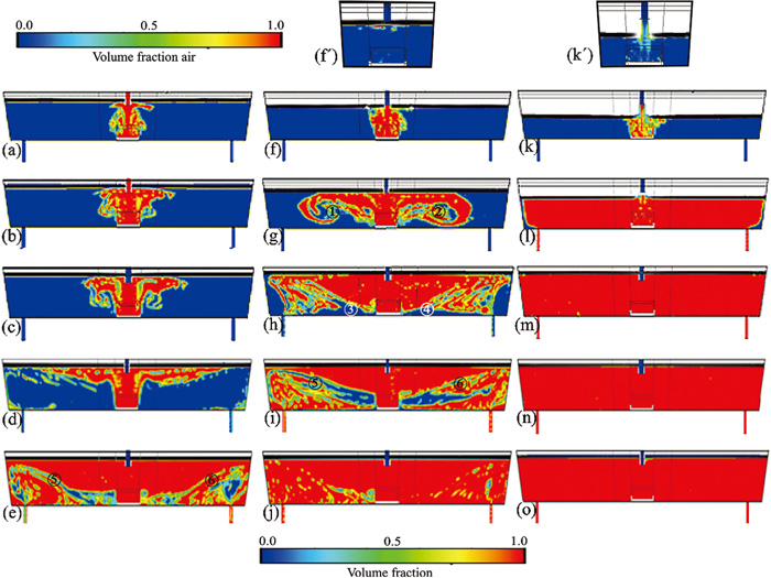
Fig. 9. New steel evolution for all cases during bath level recovering. case 1: (a) 369 s, (b) 380.5 s, (c) 400 s, (d) 500 s and (e) 740 s; case 2: (f) 429 s, (g) 485 s, (h) 549 s, (i) 649 s and (j) 849 s; case 3: (k) 533 s, (l) 637 s, (m) 740 s, (n) 840 s, (o) 1040 s, and (f´) dragged air by steel jet at 429 s for case 2, (k´) dragged air by steel jet at 533 s for case 3. (Online version in color.)

Finally, Figs. 9(k)–9(m) illustrates the evolution of the new steel for case 3; in Fig. 9(k), which corresponds to the 533 s of simulation, it is observed how the steel jet enters the tundish without the protection of the shroud inlet, opening the slag layer and allowing ambient air to enter as shown in Fig. 9(k′). Here, it is observed how the lower levels of steel air entrainment can be appreciated, generating a more intense emulsion than in case 2, causing a very disordered flow in the inlet area of the new grade of steel. Also, it is observed how the new steel flows in an upward trajectory once it hits the bottom of the inhibitor, reaching a greater path than the two previous cases due to the smaller volume of remaining old steel. Figure 9(l) illustrates how the steel at a half-level recovery has already reached the exits and almost wholly displaced the remaining old steel in the time of 637 s. At the end of the recovery stage, in this case, Fig. 9(m), the new steel has already completely displaced the remaining old steel. It flows towards the exits, beyond the fluid dynamic effect of the recirculations close to the exits, in a time of 740 s. In order to obtain a general behavior of the evolution of the new steel, this analysis was extended for each case to 100 s after the end of the level recovery (R_x) and at the end of the final steady state (F2_x). Figures 9(d) and 9(e) were acquired for case 1 at simulation times of 500 s and 740 s, respectively, and Figs. 9(i) and 9(j) for case 2 at times of 649 s and 849 s, respectively, and Figs. 9(n) and 9(o) for case 3 at times of 840 s and 1040 s, respectively. In general, it is observed that for the three cases, the new grade of steel has behaved in a very similar way upon reaching the end of this last stage, obeying the previously analyzed fluidynamics structure, with an entry and ascent of the steel in the area of input as seen in Fig. 9(d). Advancing later on the recirculations generated in the areas of the exits as seen in points ⑤ and ⑥ of Fig. 9(e) of case 1 and Fig. 9(i) of case 2, observing here the entrapment of a fraction of the old steel it will take to reach the exits. Finally, in Figs. 9(n) and 9(o) that correspond to case 3, at these simulation times, the fraction of old steel is no longer observed since, compared to the other two cases, where the volume was much lower of remaining steel that had to be moved to the exits from the start of the entry stage of the new steel.

3.4. Age Distribution Curve (Curve F) for the New Steel Grade

Figure 10 shows the evolution of the new steel at the tundish exits for each case studied, with which the type F curve was built for a change in steel grade, including case 3, under isothermal conditions. The order of appearance of the curves in the graph from left to right for all cases indicates that case 3 accumulates more simulation time than the others since it includes the longest simulated time in the emptying stage. For all cases, the criterion established for a minimum concentration (C_min) was 0.1 and 0.9 for a maximum concentration (C_max). This criterion can be adjusted depending on the degree difference between one sequence and another. In the plant, the aim is to reduce and maximize this difference. The minimum concentration indicates the lower limit of the fraction of new steel at the outputs after the start of the sequence, and the maximum concentration indicates the upper limit; this concentration range is where the manufactured steel meets the desired chemistry and what is outside of this must be discarded and reprocessed accordingly. This confidence range depends on the volume fraction of steel remaining from the old grade of steel in the tundish for each case, and, in turn, each one corresponds to a different transition time. The behavior of the curves obeys the behavior of fluid dynamics, the time required to achieve the first detection being longer for case 1 due to the greater volume of steel to be displaced, followed in that order by cases 2 and 3. Once started the detection of the new grade of steel is, the curves began their ascent with very similar slopes; however, very close to 0.8 of the dimensionless concentration, the slopes of the curves decreased. For case 1, the curve advances upward with small oscillations until reaching the dimensionless concentration of 0.9 in a longer time range (~2.91 min) than the other two cases due to the greater volume of displaced steel and the effect of the formation of recirculations near the exits.

Fig. 10. F-Curve for all studied cases. (Online version in color.)

The curve for case 2 shows a more significant slope change after the 0.8 dimensionless concentration. In this case, recirculations already exist when the new grade of steel has reached the exits. The effect they generate is: a maximum concentration peak of around 0.95 and in which path the limit concentration of ~0.9 is reached in a time range of (1.13 min), followed by a smooth descent generating a valley whose minimum value reached is ~0.88, and finally rising again very smooth up to values close to 1. The curve for case 3 shows a change in slope more significant than for the rest of the cases; after reaching 0.8 of dimensionless concentration, it reaches a maximum of ~0.98. In this course, the limit is reached 0.9 in the shorter time range than the other cases (0.4 min). After reaching the maximum peak, the concentration shows a very slight decrease to approach the value of 1 again; Thus, in this case, the low volume of old steel and the high mixing velocities generate an almost immediate chemical homogenization, reducing the effect of the recirculations already generated in the fluid dynamic structure at these times of analysis for this case. This behavior agrees with that reported by Siddiqui.¹⁴⁾ The behavior for case 3 under isothermal conditions is also shown; significant differences are observed with case 3 under non-isothermal; firstly, the slope of the isothermal case is lower, which indicates a greater range of time to reach the dimensionless concentration limits compared to its counterpart non-isothermal case, resulting in a more significant amount of intermixed steel. The other difference in the curve is that large concentration fluctuations beyond the upper limit of dimensionless concentration are not observed, which is attributed to the fact that, in this case, large recirculations are not generated on the exits, as in non-isothermal cases.

The statistical processing of the F curves allowed generating Table 2, which summarizes the critical data to calculate the intermixed steel, as well as the length of the slab that must be cut (L_cut), to ensure chemical composition specifications, for which Eq. (15) was employed. The same procedure was for both isothermal and non-isothermal conditions for case 3. Here t_Cmin, is the time where the minimum established concentration was detected and t_Cmax. is the respective time for the maximum one. The results indicate values of intermixed steel of 4.21, 1.63, 0.58, and 1.52 tons for cases 1, 2, and 3 non-isothermal and case 3 isothermal, respectively. The previous indicates that the lower the tundish level is worked with old grade steel, the shorter the transition time and, therefore, the lower the amount of intermixed steel; results with this trend have already been reported,⁴⁰⁾ hence the success of the TVF method. However, simulating the cases under isothermal conditions, the results of intermixed steel are erroneous, as observed for case 3, which has to do mainly with the fluidynamics structure developed. Considering the dimensions of the slab produced in the plant, there would be a cut length of 0.983, 0.380, 0.135, and 1.520 m for cases 1, 2, and 3 non-isothermal and case 3 isothermal, respectively. The amount of intermixed steel for the isothermal case 3 concerning its counterpart non-isothermal is 2.6 times greater. There is no doubt that the short circuit found in the fluid dynamic structure in isothermal conditions significantly affects the performance of the tundish, prolonging the delivery time of the old-grade steel, even though in case 3, there is a smaller volume of this to be displaced for the other cases.

Table 2. Statistical summary of F-curve data for all non-isothermal and isothermal cases.

Case	Steel flow per strand (ton·min−1)	Transition time (min)	t Cmin/t Cmax. (s)	Lcut (m)	Intermixed steel (ton)	Intermixed steel (% slab)
1-Non-isothermal	1.45	2.91	456/631	0.983	4.210	16.38
2-Non-isothermal	1.45	1.13	517/585	0.380	1.630	6.34
3-Non-isothermal	1.45	0.4	578/602	0.135	0.580	2.25
3-Isothermal	1.45	1.05	590/653	0.356	1.520	5.93

4. Conclusions

In the present work, the multiphase numerical simulation of a degree change was carried out in a straight-type tundish with two exits, in a non-isothermal and isothermal state, to determine the amount of intermixed steel using the TVF method, obtaining the following conclusions:

(1) The amount of remaining steel of old steel grade greatly influences the fluid dynamics structure obtained at the end of the stage of recovery of the work level of the tundish, being the greater transition towards a final quasi-steady state at higher values of this amount, as could be observed in case 1.

(2) The thermal evolution of the steel at the exits of the tundish in the numerical simulation after the grade change has been validated with plant data, finding excellent agreement in the results, with rates of temperature losses ranging between 0.42–0.44 K·min⁻¹.

(3) For steel reductions in the tundish greater than 50% during the grade change, the omission of heat transfer during the simulation affects the fluid structure is restored to the initial state, which can be classified as a loss of flow memory, generating a short circuit that prevents the steel from going to the surface, significantly affecting the amount of intermixed steel. However, in non-isothermal conditions, the effects of thermal flotation, heat loss through the walls, and drop in inlet temperature. The incorporation of the radiation model that acts in the slag opening zone is evident since they are never observed to generate a short circuit. The trend for the three cases was the same in its fluid dynamics structure at the end of the final steady state.

This mathematical model shows the importance of considering the thermal behavior of this type of inhibitor when using a 50% reduction of the old steel. Unlike other models recorded in the literature^3,14,17,19) when thermal behavior is omitted, the convection does not exist in bulk, showing the loss of flow memory for this type of inhibitor and the steel level. This phenomenon of memory loss is due to a short circuit that allows the new steel to rush out, impacting the intermixed steel. It is crucial to note that when estimating intermixed steel during a grade change through numerical models using the TVF method, one has to analyze the geometric and operational conditions of the flow modifiers and then decide to oversimplify the modeling to isothermal cases, always anticipating the usefulness and applicability of the results.

Acknowledgments

The authors want to acknowledge the CONACyT, TecNM, ITM, UMSNH and CATEDRAS CONACyT for their continuous support. The student is grateful to the CONACyT for scholarship No. 1034419 for the support of the academic degree.

References

• 1)   A. U.  Hernández,  P. G.  González,  J. A. R.  Banderas and  C. A. H.  Bocanegra: Metals, 11 (2021), 1082. https://doi.org/10.3390/met11071082
• 2)   J. E. F.  Buenrostro,  C. A. H.  Bocanegra,  J. A. R.  Banderas,  E. T.  Alonso,  N. M.  Granados and  M. R.  Argáez: Trans. Indian Inst. Met., 72 (2019), 899. https://doi.org/10.1007/s12666-018-1548-9
• 3)   D.  Mazumdar: Steel Res. Int., 90 (40) (2018), 1800279. https://doi.org/10.1002/srin.201800279
• 4)   X.  Huang,  B. G.  Thomas: Metall. Trans. B, 27B (1996), 617. https://doi.org/10.1007/BF02915660
• 5)   X.  Huang and  B. G.  Thomas: Metall. Mater. Trans. B, 24B (1993), 379. https://doi.org/10.1007/BF02659140
• 6)   M. J.  Cho and  I. C.  Kim: ISIJ Int., 46 (2006), 1416. https://doi.org/10.2355/isijinternational.46.1416
• 7)   M. J.  Cho and  S. J.  Kim: ISIJ Int., 50 (2010), 1175. https://doi.org/10.2355/isijinternational.50.1175
• 8)   R. D.  Morales,  J. P.  Ramos, J. de J. Barreto, S. L. Ramírez and D. Zacharias: Mater. Trans. B, 31B (2000), 1505. https://doi.org/10.1007/s11663-000-0035-x
• 9)   A.  Cwudziński: Int. J. Cast Met. Res., 30 (2016), 50. https://doi.org/10.1080/13640461.2016.1234223
• 10)   M. I. H.  Siddiqui and  P. K.  Jha: ISIJ Int., 54 (2014), 2578. https://doi.org/10.2355/isijinternational.54.2578
• 11)   H. J.  Odenthal,  H.  Pfeifer and  M.  Klass: Steel Res. Int., 71 (2000), 210. https://doi.org/10.1002/SRIN.200001219
• 12)   H. J.  Odenthal,  M.  Javurek,  M.  Kirschen and  N.  Vogl: Steel Res. Int., 81 (2010), 529. https://doi.org/10.1002/srin.201000079
• 13)   J. M.  Fernandez,  C. S.  Morros,  J. R.  Somoano and  M. A.  Ordieres: ASME Fluids Eng. Div. Summer Conf., Proc., 1 (2009), 2183. https://doi.org/10.1115/FEDSM2009-78353
• 14)   M. I. H.  Siddiqui and  P. K.  Jha: Steel Res. Int., 87 (2016), 733. https://doi.org/10.1002/srin.201500210
• 15)   S.  Kant,  P. K.  Jha and  P.  Kumar: Ironmak. Steelmak., 38 (2011), 391. https://doi.org/10.1179/1743281211Y.0000000007
• 16)   A.  Muralikrishna,  S.  Bagui and  D.  Mazumdar: Trans. Indian Inst. Met., 66 (2013), 281. https://doi.org/10.1007/s12666-013-0270-x
• 17)   J. H.  Ahn,  J. K.  Yoon and  J. E.  Lee: Metall. Mater. Int., 8 (2002), 271. https://doi.org/10.1007/BF03186096
• 18)   H.  Zhang,  Q.  Fang,  R.  Luo,  C.  Liu,  Y.  Wang and  H.  Ni: Metall. Trans. B, 50 (2019), 1461. https://doi.org/10.1007/s11663-019-01572-6
• 19)   M.  Alizadeh,  H.  Edris and  A. R.  Pishevar: ISIJ Int., 48 (2008), 28. https://doi.org/10.2355/isijinternational.48.28
• 20)   A. V.  Zamora,  R. D.  Morales,  M. D.  Cruz and  J. P.  Ramos: Int. J. Heat Mass Transfer., 46 (2003), 3029. https://doi.org/10.1016/S0017-9310(03)00068-1
• 21)   D. Y.  Sheng and  P. G.  Jönsson: Materials, 14 (2021), 1906. https://doi.org/10.3390/ma14081906
• 22)   S.  Chakraborty and  Y.  Sahai: ISIJ Int., 31 (1991), 960. https://doi.org/10.2355/ISIJINTERNATIONAL.31.960
• 23)   R. D.  Morales,  J. J.  Barreto,  S. L.  Ramírez,  J. P.  Ramos and  M. D.  Cruz: Modell. Simul. Mater. Sci. Eng., 8 (2000), 781. https://doi.org/10.1088/0965-0393/8/6/302
• 24)   K.  Takahashi,  M.  Ando and  T.  Ishii: ISIJ Int., 54 (2014), 304. https://doi.org/10.2355/isijinternational.54.304
• 25)   H.  Ling and  L.  Zhang: JOM, 65 (2013), 1155. https://doi.org/10.1007/s11837-013-0689-x
• 26)   H.  Ling,  L.  Zhang and  H.  Li: Metall. Mater. Trans. B, 47B (2016), 2991. https://doi.org/10.1007/s11663-016-0743-5
• 27)   H.  Ling,  R.  Xu,  H.  Wang,  L.  Chang and  S.  Qiu: ISIJ Int., 60 (2020), 499. https://doi.org/10.2355/isijinternational.ISIJINT-2019-506
• 28)   P. K.  Jha,  S. K.  Dash and  S.  Kumar: ISIJ Int., 41 (2001), 1437. https://doi.org/10.2355/isijinternational.41.1437
• 29)   H.  Zhang,  Q.  Fang,  R.  Luo,  C.  Liu,  Y.  Wang and  H.  Ni: Metall. Mater. Trans. B, 50 (2019), 1461. https://doi.org/10.1007/s11663-019-01572-6
• 30)   R. D.  Morales,  S. G.  Hernández,  J. J.  Barreto,  A.  Huerta,  I.  Ramos and  E.  Gutiérrez: Metall. Mater. Trans B, 47 (2016), 2595. https://doi.org/10.1007/s11663-016-0663-4
• 31)  Krashnavtar and D. Mazudmar: JOM, 70 (2018), 2193. https://doi.org/10.1007/s11837-018-2988-8
• 32)   Santis.  M,  Santis.  N,  Fera.  D,  Tonelli.  R,  Oktay.  S and  Oran.  A: Mater. et Tech., 107 (2020), 510.
• 33)  Kim. S and You. D., 63 (2023), 504.
• 34)   M. I. H.  Siddiqui,  M. H.  Kim: Metals, 9 (2019), 40. https://doi.org/10.3390/met9010040
• 35)  ANSYS, Inc. Fluent Theory Guide; ANSYS, Inc. (2013).
• 36)   H.  Zhang,  C.  Liu,  Q.  Fang,  Y.  Wang,  H.  Ni and  C.  Liu: Ironmak. Steelmak., 47 (2020), 1029. https://doi.org/10.1080/03019233.2019.1665909
• 37)   B. E.  Launder and  D. B.  Spalding: Comput. Methods Appl. Mech. Eng., 3 (1974), 269. https://doi.org/10.1016/0045-7825(74)90029-2
• 38)   C. E.  Grip,  L.  Jonsson,  P.  Jönsson and  K. O.  Jonsson: ISIJ Int., 39 (1999), 715. https://doi.org/10.2355/isijinternational.39.715
• 39)   O. S. D.  Ramírez,  E. T.  Alonso,  J. A. R.  Banderas,  S.  Villa and  C. A. H.  Bocanegra: Steel Res. Int., 89 (2018), 1700. https://doi.org/10.1002/srin.201700428
• 40)   B.  Bul’ko,  M.  Molnár,  P.  Demeter,  D.  Baricová and  A.  Pribulova: Metals, 8 (2018), 852. https://doi.org/10.3390/MET8100852