Assessing the Banding Degree of Martensite in the Bainite Matrix through EPMA

Abstract

Due to the difficulty of distinguishing the grain boundaries between martensite and bainite in fast-cooling microstructures, few good methods were reported to accurately assess the banding degree of martensite or bainite. In present work, a novel method has been developed to meet this challenge. The hot rolled bars of drill steel 23CrMoNi, which had martensite bands distributed in the bainite matrix, were used in this research. The banded structure in this hot rolled 23CrMoNi was closely related to the segregation of the alloying elements such as Cr, Ni and Mo. These alloying element mappings were first acquired by electron probe micro analyzer (EPMA). A new data processing method was developed to correlate the segregated element mapping with the banded structure. The banding assessment was conducted on the processed binary images of element mappings according to ASTM E1268-19. This method was well verified by assessing the banded pearlite in the ferrite matrix, whose banding degree can be easily accessed through microstructure difference. It was shown from the quantitative analysis results of the hot rolled 23CrMoNi that the banded distribution of martensite was greatly optimized by the adjustment of hot rolling process.

1. Background

Due to the selective crystallization during solidification of steel, dendrite segregation was produced inevitably in slabs, billets, or casting blanks. Thus banding of microstructure was formed after rolling process.^1,2,3) Banded microstructure in steels is the alternating bands of different microstructures, parallel to the rolling direction. The microstructuers with significant differences, such as ferrite and pearlite in hypo eutectoid steels,^2,3) can be accessed directly from their morphology features according to the standard grading charts provided in GB/T 34474.1-2017,⁴⁾ or by the quantitative method in GB/T 34474.2-2018⁵⁾ and ASTM E1268-19.⁶⁾ However the martensite and bainite bands are rarely assessed since the boundary between the bands and the matrix is difficult to distinguish.^7,8)

The present work attempted to quantitatively assess the banding degree of martensite in bainite matrix in the drill steel 23CrMoNi via the alloying element mappings, thus to evaluate the effect of the adjustment in the hot rolling procedure. A novel processing method had been proposed to extract the banded features from the element mappings, and the measurement was executed by computer according to ASTM E1268-19.⁶⁾

2. Experimental Procedure

The hot rolled bars of the drill steel 23CrMoNi were investigated in present work, on which some untypical banded features had been observed. A fast cooling process was introduced to improve its homogeneity. Samples with 20 mm in length were taken from the original bar and the adjusted bar, respectively, and were cut along their central axes. The longitudinal sections were ground and polished. The element mappings were taken from the locations at 1/4 of the diameter from surface on the polished sections, and were conducted using EPMA-1720 electron probe micro analyzer (EPMA) with a Tungsten filament gun operating at 15 kV. The electron probe parameters used were: probe current of 200 nA, spot size of 1 μm, step size of 3 μm, sampling time of 30 ms/step and scan area of 1200 μm×900 μm. After the scanning, the polished surfaces were etched with 4% nitric acid and ethanol solution, and the correspondence between the morphology and the element segregation was verified by a fast scan via EPMA-1720, and the sampling time reduced to 20 ms/step, and the scan area reduced to 600 μm×450 μm. The microstructure of the sample was observed with S-3400N tungsten filament scanning electron microscope operated with the accelerating voltage of 15 kV and the working distance of 6.4 mm.

3. Results

3.1. The Morphology of the Banded Structure

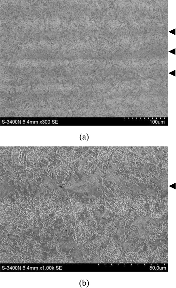
As shown in Fig. 1(a), there were some fuzzy dark bands indicated by the arrows along the rolling direction in the microstructure of the original sample. The spacing of the dark bands was roughly estimated as less than 100 μm. The micro-hardness was 424 HV0.2 in the dark bands, and 384 HV0.2 in the matrix. It can be found from Fig. 1(b), the magnified image of Fig. 1(a), that the microstructure in dark bands was mainly martensite and the matrix was mainly granular bainite. Although there were banded features, some granular bainite grains interpenetrated in the dark bands and some martensite scattered in the lighter part, so it was difficult to define the boundary between the banded feature and the matrix, and even more difficult to quantitatively assess the banded structures according to their morphology.

Fig. 1. The microstructure of hot rolled bar of the drill steel 23CrMoNi before the adjustment: (a) several dark bands indicated by the arrows could be found with the magnification of 300×; (b) the dark band was mainly martensite and the rest part was mainly granular bainite with the magnification of 1000×.

3.2. Relations between the Banded Martensite and the Element Segregation

The polished and etched sample longitudinal sections were both scanned by EPMA, respectively. On the etched section, the dark bands in the secondary electron (SE) image (Fig. 2(a)) coincided with the high concentration regions exactly in the element mapping of Cr (Fig. 2(b)), meanwhile the C mapping showed some segregation, as shown in Fig. 2(c). On the polished sample surface, the alloying elements, such as Cr, Ni and Mo, showed obvious banded segregation on the polished sample, and their high concentration regions were almost coincided, and several segregation bands went through the entire field of view, as shown in Figs. 3(a)–3(c). Since the sampling time was longer than the fast scan, the banded segregation of Cr in Fig. 3(a) was more significant than in Fig. 2(b). The scan area on the polished section was 1200 μm×900 μm, the vertical average spacing of the high concentration regions was less than 100 μm, which was consistent with the morphology in Fig. 1(a). Carbon distributed evenly throughout the field of view, besides several carbides as shown in Fig. 3(d), no segregation could be found. That indicated the segregation of carbon in the result from the etched surface might be related to the sample etching, and the carbon concentration in the martensite bands was not significantly different from the matrix with the accuracy of EPMA used. Therefore the martensite bands coincided with the high concentration regions of the alloying elements, such as Cr, Ni and Mo.

Fig. 2. The microstructure and the corresponding elements mapping in the original hot roll bar of the drill steel 23CrMoNi: (a) SE image with the magnification of 200×; (b) Cr and (c) C mappings at the same location. (Online version in color.)

Fig. 3. The elements mapping in the original hot roll bar of the drill steel 23CrMoNi: (a) Cr; (b) Ni; (c) Mo; (d) C. (Online version in color.)

After the adjustment in the hot rolling, the alloying elements, such as Cr, Ni, and Mo, still had significant banded segregation and carbon distributed evenly as shown in Fig. 4. However, the distribution of the alloying elements segregation changed: the high concentration regions became thinner and their spacing became smaller and less segregation bands going through the entire field of view.

Fig. 4. The elements mapping in the hot rolled bar of the drill steel 23CrMoNi after the adjustment: (a) Cr; (b) Ni; (c) Mo; (d) C. (Online version in color.)

The consistency of the martensite bands with the high concentration regions can be understood from the solidification process of the steel. During solidification of the liquid steel, due to the selective crystallization, dendritic growth virtually always causes some elements, such as C, S, P, Si, Mn, Cr, Ni, and Mo,^9,10) to concentrate in the inter-dendritic regions and thus leave these elements’ concentration lower in the dendritic regions, which is also called dendritic segregation. In the following reheating, hot-rolling and cooling, it is very difficult for the segregated elements except carbon to diffuse to achieve homogenization. The concentrated and depleted regions are stretched by rolling. In general the alloying elements such as Cr, Ni and Mo can increase the stability of the undercooled austenite and decrease the critical cooling rate. The lower the critical cooling rate is, the more possible it is to form martensite in stead of bainte. In the drill steel 23CrMoNi, the matensite formed in the concentrated regions while bainite formed in the depleted regions.

4. Assessing the Degree of Martensite Banding in Bainite Matrix

4.1. Transform the Mapping Data into a Binary Image

Since the difference in morphology is not significant in current samples, the standard grading charts are not suitable for the evaluation. Whereas the high concentration regions in the element mapping reveal the banded features, which can be assessed by a quantitative method as described in GB/T 34474.2-2018⁵⁾ and ASTM E1268-19.⁶⁾ Therefore the element mapping needs to be transformed in to a feature-matrix binary image. The element mapping data is essentially a matrix with the dimensions of M × N, and each number in the matrix is the concentration value of the specific element at the scanning point. The segregation of the alloying element causes the fluctuation of the values in the matrix, as Cr mapping shown in Fig. 3(a). However, the data in a element mapping is usually highly dispersed, some processing, such as the enhancement and the smooth, should be performed before defining the boundaries. The enhancement is to enlarge the difference between the high concentration regions and the other parts and the smooth is to reduce the background noise.Then the data in the mapping can be divided into two parts: the high concentration part and the background part. Then a binary image of feature-matrix can be obtained.

4.2. The Measurement on a Binary Image

As described in GB/T 34474.2-2018⁵⁾ and ASTM E1268-19,⁶⁾ a stereological measurement is used in the quantitative method, which is made by superimposing a test grid on the image of microstructure and counting the intersections and interceptions of the banded features with the test grid. Based on the intersections and interceptions, a series of results, including the number, the width, the spacing and the orientation of banded features can be calculated. Nevertheless, it is ambiguous to identify the feature interceptions at the feature boundaries, and it takes time to complete the measurement on a micrograph manually. However, for a binary image, the identification is distinct and the measurement can be performed by a computer program.

Mathematically, the binary image is a matrix of M rows and N columns composed of 0 and 1, where the background is 0 and the banded feature is 1:

  

$$f\left(x,y\right)=\{\begin{array}{c}0\\ 1\end{array}\left(i=1,2,\dots ,M;j=1,2,\dots ,N\right)$$(1)

The identification of the intersections and the interceptions turns into calculating the derivative of a row or a column in the matrix:¹¹⁾ a horizontal line in the test grid is the ith (1≤ i≤M) row in the matrix and a vertical line in the test grid is the jth (1≤ j≤N) column in the matrix. If a test line goes into or goes out of a feature, the number changes and the absolute value of first derivative will be 1, then the feature intersection number P_⊥ and P_|| can be obtained.

According to the rules of GB/T 3447.2-2018⁵⁾ and ASTM E1268-19,⁶⁾ the feature interception number N is the number of features crossed by the lines of the test grid, and there are 4 cases: 1. the test line goes through a feature, and N increases by 1; 2. the test line doesn’t touch a feature, and N doesn’t increase; 3. the test line is tangent to a feature, and N increases by 0.5; 4. the test line ends in a feature, and N increases by 0.5. For the cases 1, 2 and 4, their N exactly equals to half of P, while in case 3, it doesn’t. An auxiliary line is introduced to judge the case of tangency, and that is another test line apart with an interval of several pixels. If the feature intersection numbers on the two lines increase differently, that is the case 3, and in all cases N always equals to the half of the average value of Ps on the two lines, and then the feature interception number N_⊥ and N_|| can be obtained.

According to ASTM E1268-19,⁷⁾ the linear fraction L_L is also required, that is the fraction of a single test line on the features and it can be obtained by the ratio of the modulus to the length of the test line.

Figure 5 shows a schematic diagram of the measurement process: the image of a feature banded in horizontal direction is corresponding to a 10×10 binary matrix: the numbers in the feature is 1 and in the background is 0. A test line in horizontal direction is the 5th row indicated by the flat box in Fig. 5(b):

  

$$f\left(5,y\right)=\left[0\mathrm{\hspace{0.17em} }1\mathrm{\hspace{0.17em} }1\mathrm{\hspace{0.17em} }1\mathrm{\hspace{0.17em} }1\mathrm{\hspace{0.17em} }1\mathrm{\hspace{0.17em} }1\mathrm{\hspace{0.17em} }1\mathrm{\hspace{0.17em} }1\mathrm{\hspace{0.17em} }0\right],$$

and its first derivative is:

  

$${\frac{\partial f}{\partial y}|}_{x=5}=\left[1\mathrm{\hspace{0.17em} }0\mathrm{\hspace{0.17em} }0\mathrm{\hspace{0.17em} }0\mathrm{\hspace{0.17em} }0\mathrm{\hspace{0.17em} }0\mathrm{\hspace{0.17em} }0\mathrm{\hspace{0.17em} }0\mathrm{\hspace{0.17em} }\text{-}1\right],$$

so there are 2 intersections.

Fig. 5. Sketch of the stereological measurement on a binary image: (a) a feature image; (2) the pixelization of the feature into a 10×10 matrix.

A test line in vertical direction is the 2nd column indicated by the slender solid box in Fig. 5(b):

  

$$f\left(x,\mathrm{\hspace{0.17em} }2\right)=\left[0\mathrm{\hspace{0.17em} }0\mathrm{\hspace{0.17em} }0\mathrm{\hspace{0.17em} }0\mathrm{\hspace{0.17em} }1\mathrm{\hspace{0.17em} }1\mathrm{\hspace{0.17em} }0\mathrm{\hspace{0.17em} }0\mathrm{\hspace{0.17em} }0\mathrm{\hspace{0.17em} }0\right],$$

and its first derivative is:

  

$${\frac{\partial f}{\partial x}|}_{y=2}=\left[0\mathrm{\hspace{0.17em} }0\mathrm{\hspace{0.17em} }0\mathrm{\hspace{0.17em} }1\mathrm{\hspace{0.17em} }0-1\mathrm{\hspace{0.17em} }0\mathrm{\hspace{0.17em} }0\mathrm{\hspace{0.17em} }0\right],$$

so there are 2 intersections. Add an auxiliary line one pixel on the left to the vertical test line, indicated by the dotted box. All the pixels on the auxiliary line are 0 s and no intersection can be found. So it is a tangent hit here, and the interception number increases by 0.5. The linear fraction for the horizontal test line is 0.8 and for the vertical test line is 0.2.

After obtaining P_⊥, P_||, N_⊥, N_||, L_L⊥ and L_L|| on the whole test grid, other results can be calculated according to the rules in GB/T 34474.2-2018 and ASTM E1268-19.

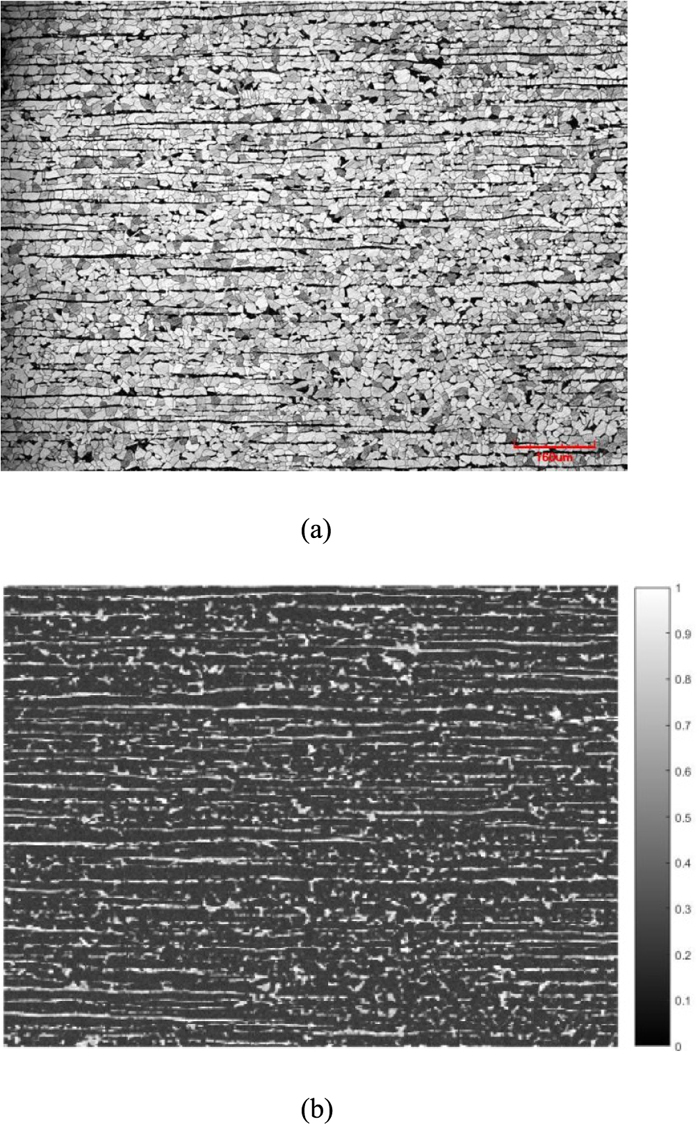
4.3. Verify the Method

Q235 steel was used to verify this method. Q235 was typical ferrite-pearlite steel, and its microstructure and element distribution had consistent banded feature. The banded structure can be clearly observed by both optical micrograph (OM) and the element mapping of C as shown in Fig. 6. The pearlite bands alternated with the ferrite bands, and the carbon concentration was high in pearlite and low in ferrite, that meant the high concentration region was exactly the pearlite band. The OM image was first measured manually, and then was processed to a binary image and measured by computer as the procedure in section 4.2. Their results were used as a standard. And the element mapping of C on the same view field was processed to a feature-matrix binary image and measured by computer, too. All the results were listed in Table 1. The consistency of the result from the element mapping with the standard results from OM verified that it was feasible to measure the banded features through the element mapping.

Fig. 6. Banded structure in Q235 steel: (a) the optical micrograph; (b) the element mapping of C of the same view field in OM. (Online version in color.)

Table 1. Assessed results of the banded structure on Q235.

	Manual result on OM	Automatic result on OM	Automatic result on element mapping
Lt||*a/mm	6.1	6.3	6.0
Lt⊥*b/mm	5.5	5.6	5.4
Nt||*c/mm	13.9	15.2	14.7
Pt||*d/mm	–	30.3	29.3
Nt⊥/mm	44.9	44.8	44.6
Pt⊥/mm	–	89.6	89.2
BR*e	–	3.452	7.265
AI*f	3.234	2.955	3.040
Ω12*g	0.587	0.554	0.565
SB⊥/μm	–	22.3	22.4
λ/μm	–	17.4	17.1

Note:

^*a:  The total length of the test lines parallel to the deformation direction.

^*b:  The total length of the test lines perpendicular to the deformation direction.

^*c:  N_t|| and N_t⊥ are the numbers of feature interceptions with test lines parallel and perpendicular to the deformation direction per unit of length, $N_{t\left|\right|}=\frac{N_{\left|\right|}}{L_{t\left|\right|}}$, $N_{t\perp }=\frac{N_{\perp }}{L_{t\perp }}$.

^*d:  P_t|| and P_t⊥ are the numbers of the feature intersections with test lines parallel and perpendicular to the deformation direction per unit of length, $P_{t\left|\right|}=\frac{P_{\left|\right|}}{L_{t\left|\right|}}$, $P_{t\perp }=\frac{P_{\perp }}{L_{t\perp }}$.

^*e:  $BR=\frac{{\sigma }_{L_{L\parallel }}}{{\sigma }_{L_{L\perp }}}$, where ${\sigma }_{L_{L\parallel }}$ and ${\sigma }_{L_{L\perp }}$ are the standard deviation in the horizontal and vertical directions, respectively.

^*f:  Since there is only one field of view, the definition of the anisotropy index (AI) in ASTM E1268-19 is adopted: $AI=\frac{N_{L\perp }}{N_{L\parallel }}$.

^*g:  ${\mathrm{\Omega }}_{12}=\frac{{\overline{N}}_{L\perp }-{\overline{N}}_{L\parallel }}{{\overline{N}}_{L\perp }+0.57{\overline{1N}}_{L\parallel }}$, ${\overline{N}}_{L\perp }$ and ${\overline{N}}_{L\parallel }$ should be the mean values of several fields of view. While for one field of view, take the measurements N_L⊥ and N_L// in the field of view instead.

4.4. Assess the Banded Structure in the Drill Steel

In the drill steel samples the segregation alloying elements were Cr, Ni and Mo, and their concentration values are highly dispersed, and the amplitude of the concentration fluctuation is much smaller than that of the contrast changing in a ferrite-pearlite microstructure image. Although several banded high concentration regions can be seen on the element mapping, the peak to background ratio is very small and it is difficult to find a continuous and closed boundary of the banded feature. The contrast profile in the illustration of Fig. 7(a) proofs that, there are too many burrs to make the stereological measurement. Therefore, it needs to enhance the signal-to-noise ratio and to reduce background noise before the binary segmentation. In present work the enhancement was achieved by multiplying every number in the matrix by a coefficient, and the value of the coefficient is linearly related to its neighbour point in the horizontal direction as shown in Fig. 7(b). So that the difference between the high concentration regions and the other parts could be enlarged, meanwhile the vertical size of them would not be affected. Then the matrix was smoothed by a median filter, and linearly mapped to a new greyscale map. After the enhancement and the smooth, every peak strictly corresponded to a centre of segregation region. Statistics of the profiles during the image processing were recorded in Table 2.

Fig. 7. The image processing on the Cr concentration mapping of the original sample: (a) the raw data was mapped to greyscale map; (b) enhanced; (c) median filtered with a 5×5 template; (d) contrast stretching. The illustrated profiles on the right showed the contrast fluctuation at the position 1/4 from the left perpendicular to the rolling direction.

Table 2. Statistics of the profiles at every stage of the image processing.

Contrast	Max.	Mean	Δmax	Number of peaks
Raw map	255	145	110	97
Enhanced	255	96	159	98
Smoothed	172	95	77	11
Contrast stretching	255	99	156	11

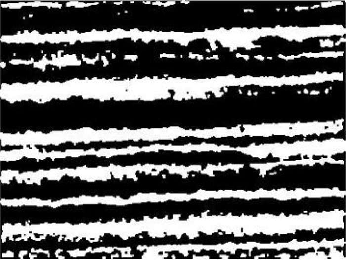
Otsu method was used on the processed greyscale maps of every alloying element like Fig. 7(d), to obtain the threshold for the binary segmentation. The high concentration regions were the target and the other parts were the background. Due to the large dispersion of the mapping data, the boundary in the binary image still had a large number of non-banded features such as burrs and holes. Therefore, the operations such as closing holes and opening holes were applied on the binary image to obtain smooth feature contours as shown in Fig. 8.

Fig. 8. The binary image of the banded features processed from Cr mapping in the original sample.

The element mappings of the original and adjusted samples were possessed to feature-matrix binary images and the banded structures were assessed according to GB/T 34474.2-2018⁵⁾ and ASTM E1268-19⁶⁾ by computer. The quantitative results were listed in Table 3. In the original sample, the mean center-to-center spacing of the bands SB_⊥ of every element was in the range of 80 μm–100 μm; the mean free path λ, that was the mean edge-to-edge spacing of the bands, showed some differences: it was 46 μm for Cr and Ni, and 64.8 μm for Mo, nearly 40% more than the former. It indicated that the element Mo had thinner high concentration regions. The anisotropy index (AI) and the degree of orientation (Ω₁₂) reflected the orientation of the banded structure, when the features were equiaxed, AI would be 1 and Ω₁₂ would be 0, and the values increased when the elongation along the rolling direction increased. For the original sample, AI’s of all the element mappings were: 2.98 (Cr), 3.12 (Ni) and 2.87 (Mo), and Ω₁₂’s were: 0.56 (Cr), 0.58 (Ni) and 0.54 (Mo), and they both indicated high orientation of the banded features. The banding rate (BR) reflected the distribution of high concentration regions: a small BR value corresponded to uniform distribution along the rolling direction. For the element mappings in Fig. 3 the BR values were quite large and that meant less alternating of the high and low concentration regions and heavier elongation in the rolling direction.

Table 3. Assessed results of the banded structure on the element mappings.

	Original			After adjustment
	Cr	Ni	Mo	Cr	Ni	Mo
Lt||/mm	7.2	7.2	7.2	7.2	7.2	7.2
Lt⊥/mm	5.4	5.4	5.4	5.4	5.4	5.4
NL||/mm	3.9	4.0	3.5	10.3	10.8	10.0
PL||/mm	7.8	7.9	7.0	20.6	21.5	20.0
NL⊥/mm	11.6	12.4	10.0	19.5	20.0	18.0
PL⊥/mm	23.1	24.7	20.1	39.1	39.9	36.0
BR	13.2	19.2	9.9	3.8	2.5	2.7
AI	2.98	3.12	2.87	1.90	1.85	1.80
Ω12	0.56	0.58	0.54	0.36	0.35	0.34
SB⊥/μm	86.4	80.9	99.5	51.2	50.1	55.5
λ/μm	46.3	46.0	64.8	32.5	30.6	37.0

The segregation ratio (SR)¹²⁾ of a specific element can be calculated according to

  

$$S{R}_X=\frac{C_{max}}{C_{min}}$$(2)

where X indicated the amount of data used for calculation. In present work, take X = 15, i.e. to take the arithmetic average value of the least 15% data as the minimum value C_min of the specified element concentration, and to take the arithmetic average value of the maximal 15% data as the maximum value C_max. The results of segregation ratio were listed in Table 4, and it showed that though the concentration of Mo is one order of magnitude lower than the other two elements, its segregation ratio was heavier than them. And the concentrations of Cr and Ni were similar and so were the segregation ratios. The enrichment of Cr, Ni and Mo would reduce the critical cooling rate during quenching, and improve the hardenability of the material, and contribute to the formation of martensite.¹³⁾

Table 4. The segregation ratio of the elements in the hot rolled bars before and after the adjustment (X = 15).

Element	Original			After adjustment
	Cmin	Cmax	SR15	Cmin	Cmax	SR15
Cr	1.58	2.41	1.52	1.82	2.64	1.45
Ni	2.57	3.63	1.41	2.60	3.62	1.39
Mo	0.10	0.39	3.88	0.13	0.43	3.45

In the adjusted sample the mean center-to-center spacing of the bands SB_⊥ of every element was in the range of 50 μm–56 μm, and the mean free path λ reduced as well. The AI, Ω₁₂ and BR reduced to 1.80–1.90, 0.34–0.36 and 2.5–3.7, respectively. That meant the size of the high concentration regions along the rolling direction was reduced, in other words, the bands became shorter. Moreover, the high and low concentration regions alternated more frequently and the distribution was more uniform.

The segregation ratios of each element were still calculated with X = 15, and the results were listed in Table 4. It could be seen from the comparison that the segregation ratios of each element after the adjustment were only slightly decreased. That indicated that the adjustment didn’t significantly promote the diffusion of alloying elements, since the diffusion rate of the alloying elements such as Cr, Ni and Mo was very slow and there was not enough time during the hot rolling for them to fully reduce the segregation.¹⁾ Therefore, the probability of martensite transformation still existed.

According to the quantitative results of the segregation ratio and banded structure of the alloying element mappings, it could be seen that although the adjustment of the rolling process cannot significantly improve the uniformity of the alloying elements, the spatial distribution of the segregation bands had been greatly optimized and the uniformity of the microstructure had been promoted.

5. Conclusion

In this work, a new processing method on the element segregation was provided, to give a quantitative analysis on the banded structure of the drill steel 23CrMoNi. The following conclusions were obtained:

(1) The banded structure can be revealed by maps of alloying elements.The banded structure in the hot rolled bars of the drill steel 23CrMoNi was closely related to the segregation of the alloying elements such as Cr, Ni and Mo. The locations of high concentration region of these three elements were nearly coincident, and consisted with the martensite bands of the microstructure. The enrichment of these alloying elements in bands led to the enhancement of local hardenability and thus the formation of martensite.

(2) The alloying elements’ maps can be quantitatively analyzed to obtain the degree of banding according to ASTM 1268-19. Through the newly developed data processing method, the feature-matrix binary images were obtained from the alloying elements’ maps.Therefore, the stereological measurement, based on ASTM 1268-19, can be easily executed automatically on these binary images.

(3) The quantitative analysis results showed that the rolling process adjustment slightly decreased segregation of alloying elements in hot rolled bars, while the spatial distribution of segregation bands had been significantly optimized, that was, the size and elongation of the bands were reduced, the anisotropy and the orientation of banded structure were weakened, and the microstructure uniformity was improved.

References

• 1)   G.  Krauss: Metall. Mater. Trans. B, 34 (2003), 781. https://doi.org/10.1007/s11663-003-0084-z
• 2)   J. D.  Verhoeven: J. Mater. Eng. Perform., 9 (3) (2000), 286. https://doi.org/10.1361/105994900770345935
• 3)   R. A.  Grange: Metall. Mater. Trans. B, 2 (2) (1971), 417. https://doi.org/10.1007/BF02663328
• 4)  GB/T 34474.1-2017, Determination of banded structure of steel—Part1: Micrographic method using standards diagrams (in Chinese).
• 5)  GB/T 34474.2-2018, Determination of banded Structure of steel - Part 2: Quantitative method (in Chinese).
• 6)  ASTM E1268-19, Standard Practice for Assessing the Degree of Banding or Orientation of Microstructures.
• 7)   A.  Ramazani,  H.  Quade,  M.  Abbasi and  U.  Prahl: Mater. Sci. Eng. A, 651 (2016), 160. https://doi.org/10.1016/j.msea.2015.10.111
• 8)   F. G.  Caballero,  A.  García-Junceda,  C.  Capdevila and  C.  García de Andrés: Mater. Trans., 47 (9) (2006), 2269. https://doi.org/10.2320/matertrans.47.2269
• 9)   Y.  Wang,  Y.  Chen and  W.  Yu: Int. J Min. Met. Mater., 28 (4) (2021), 665. https://doi.org/10.1007/s12613-020-2035-y
• 10)   C.  Yang,  Y. A.  Min,  H. P.  Sun,  T.  Gu and  J. M.  Fu: Adv. Mater. Res., 915–916 (2014), 643. https://doi.org/10.4028/www.scientific.net/amr.915-916.643
• 11)   X. L.  Meng: Physical Testing and Chemical Analysis Part A:Physical Testing, 55 (9) (2019), 598 (in Chinese).
• 12)  ISO 23692: 2021, Microbeam analysis — Electron probe microanalysis — Quantitative analysis of Mn dendritic segregation in continuously cast steel product.
• 13)   M.  Zhao,  T.  Unenbayar,  Y.  Zhao,  C.  Liu,  Y.  Tian,  D.  Yin and  A.  Atrens: Steel Res. Int., 90 (12) (2019), 1900297. https://doi.org/10.1002/srin.201900297