Carbon dioxide and water in the crust. Part 1: Equation of state for the fluid

Abstract

H₂O-CO₂-dominated fluids play a crucial role in most geological phenomena involving fluid-mineral-melt interactions. The equation of state is an essential tool for understanding the phenomena because it predicts the thermodynamic properties of the fluids. The modified Lee-Kesler equation of state for H₂O-CO₂ mixture fluid developed by Duan and Zhang (2006) is the most accurate at present and is applicable to a wide pressure-temperature range (∼ 2573 K and ∼ 10 GPa). Because of its high accuracy and wide applicable range, the equation has been used for constructing solubility laws in silicate melts. In this paper I review the Duan and Zhang (2006) equation of state and present the calculation procedure. Because the equation for calculating the partial fugacity coefficient is erroneously presented in the original paper, the correct equation is provided here. A C-language code and a Windows executable program for computing thermodynamic properties are provided for the convenience of users. The influence of the nonideal behaviour of the H₂O-CO₂ mixture fluid on some geological situations is discussed.

INTRODUCTION

The H₂O-CO₂ fluid is one of the important constituents in the crust. The fluid plays a crucial role in various geological phenomena including magma generation and differentiation, metamorphism, metasomatism, ore formation, and volcanic eruption, because the fluid changes phase relations and acts as a medium for effective transport of the thermal energy and chemical components (e.g., Ferry and Baumgartner, 1987; Holloway, 1987). To understand the phenomena, quantification of the thermodynamic properties of the fluid is essential.

An equation of state is a powerful tool to estimate the pressure-temperature-volume relations and thermodynamic properties of the fluid (e.g., Chapter 13 of Anderson, 2005; Gottschalk, 2007). The equation of state can be classified into two types: the Redlich-Kwong-type equation and the virial-type equation (e.g., Chapter 1 of Walas, 1985; Chapter 2 of Nordstrom and Munoz, 1994; Shibue, 1995; Chapter 13 of Anderson, 2005). The former is an extension of the van der Waals equation and has a limited number of parameters. Therefore the calculation is relatively easily performed and thus the Redlich-Kwong-type equation is favoured in many studies. For the H₂O-CO₂ fluid, the modified Redlich-Kwong (MRK) equation has been developed extensively for use in geological studies. The MRK equations of Holloway (1977) and Kerrick and Jacobs (1981) have been most widely used in petrological studies. The Holloway (1977) equation was then corrected by Flowers (1979). These equations were calibrated with experimental pressure-temperature-volume data, and the applicable pressure-temperature range is 450-1800 °C and 0.5-40 kbar for the equation by Holloway (1977) and ∼ 1000 °C and ∼ 30 kbar for the equation by Kerrick and Jacobs (1981).

The virial-type equation provides the compressibility factor (compression factor) as a polynomial equation of the volume (or density) terms. The number of parameters for the virial-type equation is much larger than those used in the Redlich-Kwong-type equations, and the calculation requires tasks. The virial-type equation was originally developed as a purely empirical equation in the earlier studies, but later physical meanings of the parameters were provided based on statistical mechanical analysis (Chapter 1 of Walas, 1985). Because the infinite series of the virial expansion is impractical for use, the polynomial equation is usually truncated at the several-order term. Some equations have an additional exponential term that acts as a catch-all for the missing terms. A modern successful equation of this type includes the Lee-Kesler equation (Lee and Kesler, 1975; See APPENDIX for detail), which has been mainly used for hydrocarbons in industry. For the H₂O-CO₂ fluid, Duan and coworkers in the 1990s began to develop a highly accurate equation by extending the Lee-Kesler equation. First, Duan et al. (1992a) developed an equation of state for pure H₂O, CO₂, and CH₄ at 0-1000 °C and 0-800 MPa. Duan et al. (1992b) then introduced mixing rules into the equation of state and extended its applicability to the mixture of H₂O-CO₂-CH₄ at 50-1000 °C and 0-100 MPa. Duan et al. (1992c, 1995) performed a molecular dynamics (MD) simulation to estimate the volume at high-pressure conditions because experimental determination for pressure-temperature-volume data at higher pressures is difficult and no more experiments are expected to be done. Using the MD simulation results, Duan et al. (1992c, 1996) developed a widely applicable equation for CO₂, N₂, CO, H₂, O₂, Cl₂ (Duan et al., 1992c) and H₂O-CO₂-CH₄-N₂-CO-H₂-O₂-H₂S-Ar systems (Duan et al., 1996). Finally, Duan and Zhang (2006) carried out ab initio simulation and obtained 690 points of pressure-temperature-volume data, through which the equation of state for H₂O-CO₂ mixtures applicable up to ∼ 10 GPa and 673.15-2573.15 K was developed. At present, this equation of state seems to be the most accurate for H₂O-CO₂ fluids, and it is applied to the H₂O-CO₂ solubility model for silicate melts (Duan, 2014; Ghiorso and Gualda, 2015), as reviewed in Part 2 (Yoshimura, 2023).

The present study (Part 1) reviews the equation of state for the H₂O-CO₂ mixture fluid developed by Duan and Zhang (2006). The following items are reviewed in this order: 1) the general mathematical form of the equation of state, 2) explicit equations for fugacity coefficient for pure and mixed fluids, 3) general characteristics of the molar volume and activity coefficient, and the comparison with the equation of state by Kerrick and Jacobs (1981). In addition, 4) the importance of nonideal mixing in geological situations where two fluids mix is discussed. It is cautioned that equations for the partial fugacity coefficient are erroneously presented in Duan’s papers. The correct equation is therefore presented in this paper. An example computer code written in the C-language and a Windows executable program are also provided as Supplementary Material (available online from https://doi.org/10.2465/jmps.221224a) so that readers can easily reproduce the correct calculations for the thermodynamic properties of the fluid.

THE MODIFIED LEE-KESLER EQUATION OF STATE FOR H₂O-CO₂ FLUID

Duan and Zhang (2006) used the modified version of the Lee-Kesler equation (Lee and Kesler, 1975). The original Lee-Kesler equation is briefly reviewed in the APPENDIX A. The modified Lee-Kesler equation for geological fluids was first formulated by Duan et al. (1992a, 1992b), and the parameters used therein were updated by Duan and Zhang (2006) so that the equation can be applicable to wider pressure-temperature conditions.

The modified Lee-Kesler equation is given as:

  

\begin{align} Z &= \frac{PV_{\text{m}}}{RT} = 1 + \frac{BV_{\text{c}}}{V_{\text{m}}} + \frac{CV_{\text{c}}^{2}}{V_{\text{m}}^{2}} + \frac{DV_{\text{c}}^{4}}{V_{\text{m}}^{4}} \\&\quad+ \frac{EV_{\text{c}}^{5}}{V_{\text{m}}^{5}} + \frac{FV_{\text{c}}^{2}}{V_{\text{m}}^{2}}\left(\beta + \frac{\gamma V_{\text{c}}^{2}}{V_{\text{m}}^{2}}\right) \exp\left(-\frac{\gamma V_{\text{c}}^{2}}{V_{\text{m}}^{2}}\right) \end{align} (1),

where Z is the compressibility factor (a non-dimensional value), P is the pressure (bar), V_m is the molar volume (cm³ mol⁻¹), R is the gas constant (83.14467 bar cm³ K⁻¹ mol⁻¹), and T is the temperature (K). The parameters B, C, D, E, and F are functions of temperature and are given as:

  

\begin{equation} B = a_{1} + a_{2}\left(\frac{T_{\text{c}}}{T}\right)^{2} {}+ a_{3}\left(\frac{T_{\text{c}}}{T}\right)^{3} \end{equation} (2a),

  

\begin{equation} C = a_{4} + a_{5}\left(\frac{T_{\text{c}}}{T}\right)^{2} {}+ a_{6}\left(\frac{T_{\text{c}}}{T}\right)^{3} \end{equation} (2b),

  

\begin{equation} D = a_{7} + a_{8}\left(\frac{T_{\text{c}}}{T}\right)^{2} {}+ a_{9}\left(\frac{T_{\text{c}}}{T}\right)^{3} \end{equation} (2c),

  

\begin{equation} E = a_{10} + a_{11}\left(\frac{T_{\text{c}}}{T}\right)^{2} {}+ a_{12}\left(\frac{T_{\text{c}}}{T}\right)^{3} \end{equation} (2d),

and

  

\begin{equation} F = \alpha\left(\frac{T_{\text{c}}}{T}\right)^{3} \end{equation} (2e).

The parameters β and γ in Eq. (1) and a₁, a₂, …, a₁₂, and α in Eq. (2a)-(2e) are constant values dependent on volatile species (H₂O or CO₂) and pressure conditions (Table 1): when the pressure is 0-0.2 GPa, the low-pressure values are used, whereas when the pressure is 0.2-10 GPa, the high-pressure values are used. T_c is the critical temperature (647.25 K for H₂O and 304.1282 K for CO₂). V_c in Eq. (1) is given as:

  

\begin{equation} V_{\text{c}} = \frac{RT_{\text{c}}}{P_{\text{c}}} \end{equation} (3),

where P_c is the critical pressure (221.19 bar for H₂O and 73.773 bar for CO₂). At a given temperature and pressure, V_m is obtained by solving Eq. (1) numerically based on some techniques such as the Newton-Raphson method (e.g., Chapter 3 of Albarède, 1995).

Table 1. Values for parameters in Eqs. (1) and (2a)-(2e)

Parameters	H2O		CO2
	0-0.2 GPa	0.2-10 GPa	0-0.2 GPa	0.2-10 GPa
a1	4.38269941 × 10−2	4.68071541 × 10−2	1.14400435 × 10−1	5.72573440 × 10−3
a2	−1.68244362 × 10−1	−2.81275941 × 10−1	−9.38526684 × 10−1	7.94836769
a3	−2.36923373 × 10−1	−2.43926365 × 10−1	7.21857006 × 10−1	−3.84236281 × 101
a4	1.13027462 × 10−2	1.10016958 × 10−2	8.81072902 × 10−3	3.71600369 × 10−2
a5	−7.67764181 × 10−2	−3.86603525 × 10−2	6.36473911 × 10−2	−1.92888994
a6	9.71820593 × 10−2	9.30095461 × 10−2	−7.70822213 × 10−2	6.64254770
a7	6.62674916 × 10−5	−1.15747171 × 10−5	9.01506064 × 10−4	−7.02203950 × 10−6
a8	1.06637349 × 10−3	4.19873848 × 10−4	−6.81834166 × 10−3	1.77093234 × 10−2
a9	−1.23265258 × 10−3	−5.82739501 × 10−4	7.32364258 × 10−3	−4.81892026 × 10−2
a10	−8.93953948 × 10−6	1.00936000 × 10−6	−1.10288237 × 10−4	3.88344869 × 10−6
a11	−3.88124606 × 10−5	−1.01713593 × 10−5	1.26524193 × 10−3	−5.54833167 × 10−4
a12	5.61510206 × 10−5	1.63934213 × 10−5	−1.49730823 × 10−3	1.70489748 × 10−3
α	7.51274488 × 10−3	−4.49505919 × 10−2	7.81940730 × 10−3	−4.13039220 × 10−1
β	2.51598931	−3.15028174 × 10−1	−4.22918013	−8.47988634
γ	3.94000000 × 10−2	1.25000000 × 10−2	1.58500000 × 10−1	2.80000000 × 10−2

Reproduced from Table 4 of Duan and Zhang (2006).

MIXING RULES

To apply Eq. (1) to H₂O-CO₂ binary mixture fluid, mixing rules are necessary. Duan et al. (1992b), after trial and error, found that the mixing rules that have the virial-expansion form similar to those of Anderko and Pitzer (1991) well reproduce the experimental data. The same rules are also employed in the equation of state by Duan and Zhang (2006).

For the H₂O-CO₂ binary mixture fluid with the H₂O mole fraction of y₁ and CO₂ mole fraction of y₂ (i.e., y₁ + y₂ = 1) (hereafter subscripts 1 and 2 attached to parameters represent those of H₂O and CO₂, respectively), the mixing rules are given as follows:

  

\begin{equation} BV_{\text{c}} = \sum_{i=1}^{2}\sum_{j=1}^{2}y_{i}y_{j}B_{ij}{V_{\text{c}}}_{\,ij} \end{equation} (4a),

  

\begin{equation} CV_{\text{c}}^{2} = \sum_{i=1}^{2}\sum_{j=1}^{2}\sum_{k=1}^{2}y_{i}y_{j}y_{k}C_{ijk}{V_{\text{c}}^{2}}_{ijk} \end{equation} (4b),

  

\begin{equation} DV_{\text{c}}^{4} = \sum_{i=1}^{2}\sum_{j=1}^{2}\sum_{k=1}^{2}\sum_{l=1}^{2}\sum_{m=1}^{2}y_{i}y_{j}y_{k}y_{l}y_{m}D_{ijklm}{V_{\text{c}}^{4}}_{ijklm} \end{equation} (4c),

  

\begin{equation} {EV_{\text{c}}^{5} = \sum_{i=1}^{2}\sum_{j=1}^{2}\sum_{k=1}^{2}\sum_{l=1}^{2}\sum_{m=1}^{2}\sum_{n=1}^{2}y_{i}y_{j}y_{k}y_{l}y_{m}y_{n}E_{ijklmn}{V_{\text{c}}^{5}}_{ijklmn}} \end{equation} (4d),

  

\begin{equation} FV_{\text{c}} = \sum_{i=1}^{2}\sum_{j=1}^{2}y_{i}y_{j}F_{ij}{V_{\text{c}}}_{\,ij} \end{equation} (4e),

  

\begin{equation} \beta = \sum_{i=1}^{2}y_{i}\beta_{i} \end{equation} (4f),

and

  

\begin{equation} \gamma V_{\text{c}}^{2} = \sum_{i=1}^{2}\sum_{j=1}^{2}\sum_{k=1}^{2}y_{i}y_{j}y_{k}\gamma_{ijk}{V_{\text{c}}^{2}}_{ijk} \end{equation} (4g),

wherein the parameters for the mixture are given as follows:

  

\begin{equation} B_{ij} = \left(\frac{\root 3 \of {B_{i}} + \root 3 \of {B_{j}}}{2}\right)^{3}k_{1,ij} \end{equation} (5a),

  

\begin{equation} {V_{\text{c}}}_{\,ij} = \left(\frac{\root 3 \of {{V_{\text{c}}}_{\,i}} + \root 3 \of {{V_{\text{c}}}_{\,j}}}{2}\right)^{3} \end{equation} (5b),

  

\begin{equation} C_{ijk} = \left(\frac{\root 3 \of {C_{i}} + \root 3 \of {C_{j}} + \root 3 \of {C_{k}}}{3}\right)^{3}k_{2,ijk} \end{equation} (5c),

  

\begin{equation} {V_{\text{c}}}_{\,ijk} = \left(\frac{\root 3 \of {{V_{\text{c}}}_{\,i}}+ \root 3 \of {{V_{\text{c}}}_{\,j}}+\root 3 \of {{V_{\text{c}}}_{\,k}}}{3}\right)^{3} \end{equation} (5d),

  

\begin{equation} D_{ijklm} = \left(\frac{\root 3 \of {D_{i}} + \root 3 \of {D_{j}} + \root 3 \of {D_{k}} + \root 3 \of {D_{l}} + \root 3 \of {D_{m}}}{5}\right)^{3} \end{equation} (5e),

  

\begin{equation} {V_{\text{c}}}_{\,ijklm} = \left(\frac{\root 3 \of {{V_{\text{c}}}_{\,i}} + \root 3 \of {{V_{\text{c}}}_{\,j}} + \root 3 \of {{V_{\text{c}}}_{\,k}} + \root 3 \of {{V_{\text{c}}}_{\,l}} + \root 3 \of {{V_{\text{c}}}_{\,m}}}{5}\right)^{3} \end{equation} (5f),

  

\begin{equation} E_{ijklmn} = \left(\frac{\root 3 \of {E_{i}} + \root 3 \of {E_{j}} + \root 3 \of {E_{k}} + \root 3 \of {E_{l}} + \root 3 \of {E_{m}} + \root 3 \of {E_{n}}}{6}\right)^{3} \end{equation} (5g),

  

\begin{align} &{{V_{\text{c}}}_{\,ijklmn}} \\&\quad = {\left(\frac{\root 3 \of {{V_{\text{c}}}_{\,i}} + \root 3 \of {{V_{\text{c}}}_{\,j}} + \root 3 \of {{V_{\text{c}}}_{\,k}} + \root 3 \of {{V_{\text{c}}}_{\,l}} + \root 3 \of {{V_{\text{c}}}_{\,m}} + \root 3 \of {{V_{\text{c}}}_{\,n}}}{6}\right)^{3}} \end{align} (5h),

  

\begin{equation} F_{ij} = \left(\frac{\root 3 \of {F_{i}} + \root 3 \of {F_{j}}}{2}\right)^{3} \end{equation} (5i),

and

  

\begin{equation} \gamma_{ijk} = \left(\frac{\root 3 \of {\gamma_{i}} + \root 3 \of {\gamma_{j}} + \root 3 \of {\gamma_{k}}}{3}\right)^{3}k_{3,ijk} \end{equation} (5j).

The mixing calculation is performed as follows. First, values for parameters B, C, D, E, and F as well as β and γ for the pure H₂O and CO₂ fluid are obtained based on Eqs. (2a)-(2e) and Table 1. V_c and V_m for the pure H₂O and pure CO₂ are also calculated with Eq. (3) and (1), respectively. Subscripts 1 and 2 are attached to the parameters for these values (for example, B for pure H₂O is set as B₁ and B for pure CO₂ is set as B₂). Next, parameters for the mixture are calculated according to Eq. (5a)-(5j). For example, B₁₂ (= B₂₁) is obtained with B₁, B₂, and Eq. (5a). Similarly, C₁₁₂ (= C₁₂₁ = C₂₁₁) and C₁₂₂ (= C₂₁₂ = C₂₂₁) are calculated according to Eq. (5c). Other mixture parameters are also calculated in the same manner. In the case that all subscripts are identical (i = j; i = j = k), the parameter represents that for the pure fluid. For example, B₁₁ is identical to B₁ and B₂₂ is identical to B₂. Similarly, C₁₁₁ is identical to C₁ and C₂₂₂ is identical to C₂. Then, the terms BV_c, $CV_{\text{c}}^{2}$, … for the mixture are calculated with Eq. (4a)-(4g). Note that the terms BV_c, $CV_{\text{c}}^{2}$, … are not simple products of two parameters: for example, BV_c is not a product of B and V_c, but is calculated as $BV_{\text{c}} = y_{1}^{2}B_{1}V_{\text{c}\,1} + 2y_{1}y_{2}B_{12}V_{\text{c}\,12} + y_{2}^{2}B_{2}V_{\text{c}\,2}$ according to Eq. (4a). Finally, putting all these parameters in Eq. (1), Z and V_m for the mixture are calculated. A numerical technique such as the Newton-Raphson method is again used for this calculation.

In Eqs. (5a), (5c), and (5j), the terms k_1,ij, k_2,ijk, and k_3,ijk denote binary interaction parameters dependent on the temperature and pressure range and interacting components (Table 2). For example, for k_1,ij, when i ≠ j (i.e., k_1,12 = k_1,21), k_1,ij is 3.131 − 5.6024 × 10⁻³T + 1.8641 × 10⁻⁶T² − 31.409/T where T represents temperature (K) if the pressure is 0-0.2 GPa, whereas it is 9.034 − 7.9212 × 10⁻³T + 2.3285 × 10⁻⁶T² − 2.4221 × 10³/T if the pressure is 0.2-10 GPa. When i = j (k_1,11 = k_1,22), k_1,ij is 1 irrespective of temperature and pressure range. Similar rules apply to k_2,ijk and k_3,ijk.

Table 2. Binary interaction parameters

Pressure range	Parameters	Conditions for i, j, and k	Equation(1)
0-0.2 GPa	k1,ij	i ≠ j	3.131 − 5.0624 × 10−3 × T + 1.8641 × 10−6 × T2 − 31.409 × T−1
		i = j	1
	k2,ijk	i ≠ j ≠ k, i = j ≠ k, j = k ≠ i	−46.646 + 4.2877 × 10−2 × T − 1.0892 × 10−5 × T2 + 1.5782 × 104 × T−1
		i = j = k	1
	k3,ijk	i ≠ j ≠ k, i = j ≠ k, j = k ≠ i	0.9
		i = j = k	1
0.2-10 GPa	k1,ij	i ≠ j	9.034 − 7.9212 × 10−3 × T + 2.3285 × 10−6 × T2 − 2.4221 × 103 × T−1
		i = j	1
	k2,ijk	i ≠ j ≠ k, i = j ≠ k, j = k ≠ i	−1.068 + 1.8756 × 10−3 × T − 4.9371 × 10−7 × T2 + 6.6180 × 102 × T−1
		i = j = k	1
	k3,ijk	i ≠ j ≠ k, i = j ≠ k, j = k ≠ i	1
		i = j = k	1

Reproduced from Table 6 of Duan and Zhang (2006).

⁽¹⁾T represents the temperature (K) and its range is 673.15-2573.15 K.

FUGACITY COEFFICIENT OF PURE FLUID

Calculation of the fugacity coefficient is essential to evaluate phase equilibrium because it is directly related to the chemical potential. For a pure fluid (H₂O or CO₂), the fugacity coefficient ϕ is defined as:

  

\begin{equation} \phi = \frac{f}{P} \end{equation} (6),

where f is the fugacity. The fugacity coefficient is obtained from the equation of state as (Chapter 3 of Walas, 1985):

  

\begin{equation} \ln \phi = Z - 1 - \ln Z - \frac{1}{RT}\int_{\infty}^{V}\left(P - \frac{RT}{V}\right)dV \end{equation} (7),

where V represents the volume of the fluid. Using Eq. (1) and (7) and assuming 1 mol of fluid (V → V_m), the following equation is obtained:

  

\begin{align} \ln \phi &= Z - 1 - \ln Z + \frac{BV_{\text{c}}}{V_{\text{m}}} + \frac{CV_{\text{c}}^{2}}{2V_{\text{m}}^{2}} + \frac{DV_{\text{c}}^{4}}{4V_{\text{m}}^{4}} + \frac{EV_{\text{c}}^{5}}{5V_{\text{m}}^{5}} \\ & \quad + \frac{F}{2\gamma}\left[\beta + 1 - \left(\beta + 1 + \frac{\gamma V_{\text{c}}^{2}}{V_{\text{m}}^{2}}\right)\exp\left(-\frac{\gamma V_{\text{c}}^{2}}{V_{\text{m}}^{2}}\right)\right] \end{align} (8).

Note that this equation is not shown in Duan and Zhang (2006) but is provided in Duan et al. (1992a) and the Appendix of Duan (2014).

PARTIAL FUGACITY COEFFICIENT IN A FLUID MIXTURE

The partial fugacity coefficient of a component i in a mixture fluid, ϕ_i, is defined as:

  

\begin{equation} \phi_{i} = \frac{f_{i}}{y_{i}P} \end{equation} (9),

where y_iP represents the partial pressure and f_i represents the partial fugacity of component i. The partial fugacity coefficient is given as (Chapter 3 of Walas, 1985; Chapter 3 of Prausnitz et al., 1999):

  

\begin{equation} \ln \phi_{i} = \frac{1}{RT}\int_{0}^{P}\left(\bar{V_{i}} - \frac{RT}{P}\right)dP \end{equation} (10),

where $\bar{V_{i}}$ represents the partial molar volume of component i in the mixture fluid. Eq. (10) can be transformed into the following form (Chapter 3 of Walas, 1985; Chapter 3 of Prausnitz et al., 1999):

  

\begin{equation} \ln \phi_{i} = \frac{1}{RT}\int_{\infty}^{V}\left[\left(\frac{\partial P}{\partial n_{i}}\right)_{T,V,n_{j}} {}- \frac{RT}{V} \right]dV - \ln Z \end{equation} (11),

where n_i and n_j represent the amount of substance for H₂O or CO₂. Applying Eq. (11) to Eq. (1), ϕ_i is obtained as:

  

\begin{align} &\ln \phi_{i} \\ & \quad= -\ln Z + \frac{(BV_{\text{c}})_{i}{'}}{V_{\text{m}}} + \frac{(CV_{\text{c}}^{2})_{i}{'}}{2V_{\text{m}}^{2}} + \frac{(DV_{\text{c}}^{4})_{i}{'}}{4V_{\text{m}}^{4}} + \frac{(EV_{\text{c}}^{5})_{i}{'}}{5V_{\text{m}}^{5}} \\ & \qquad+ \frac{(FV_{\text{c}}^{2})_{i}{'}\beta + \beta_{i}{'}FV_{\text{c}}^{2}}{2\gamma V_{\text{c}}^{2}}\left[1 - \exp\left(-\frac{\gamma V_{\text{c}}^{2}}{V_{\text{m}}^{2}}\right)\right] \\ & \qquad + {\frac{(FV_{\text{c}}^{2})_{i}{'}\gamma V_{\text{c}}^{2} + (\gamma V_{\text{c}}^{2})_{i}{'}FV_{\text{c}}^{2} - FV_{\text{c}}^{2}\beta [(\gamma V_{\text{c}}^{2})_{i}{'} - \gamma V_{\text{c}}^{2}]}{2(\gamma V_{\text{c}}^{2})^{2}}}\\ & \qquad\times \left[1 - \left(\frac{\gamma V_{\text{c}}^{2}}{V_{\text{m}}^{2}} + 1\right)\exp\left(-\frac{\gamma V_{\text{c}}^{2}}{V_{\text{m}}^{2}}\right)\right] \\ & \qquad - \frac{[(\gamma V_{\text{c}}^{2})_{i}{'} - \gamma V_{\text{c}}^{2} ]FV_{\text{c}}^{2}}{2(\gamma V_{\text{c}}^{2})^{2}}\\ & \qquad \times\left[2 - \left(\frac{(\gamma V_{\text{c}}^{2})^{2}}{V_{\text{m}}^{4}} + \frac{2\gamma V_{\text{c}}^{2}}{V_{\text{m}}^{2}} + 2\right)\exp \left(-\frac{\gamma V_{\text{c}}^{2}}{V_{\text{m}}^{2}}\right)\right] \end{align} (12),

where $(BV_{\text{c}})_{i}{}'$, $(CV_{\text{c}}^{2})_{i}{}'$, … represent the following functions:

  

\begin{equation} (BV_{\text{c}})_{i}{'} = 2\sum_{j=1}^{2}y_{j}B_{ij}{V_{\text{c}}}_{\,ij} \end{equation} (13a),

  

\begin{equation} (CV_{\text{c}}^{2})_{i}{'} = 3\sum_{j=1}^{2}\sum_{k=1}^{2}y_{j}y_{k}C_{ijk}{V_{\text{c}}^{2}}_{ijk} \end{equation} (13b),

  

\begin{equation} (DV_{\text{c}}^{4})_{i}{'} = 5\sum_{j=1}^{2}\sum_{k=1}^{2}\sum_{l=1}^{2}\sum_{m=1}^{2}y_{j}y_{k}y_{l}y_{m}D_{ijklm}{V_{\text{c}}^{4}}_{ijklm} \end{equation} (13c),

  

\begin{equation} {(EV_{\text{c}}^{5})_{i}{'} = 6\sum_{j=1}^{2}\sum_{k=1}^{2}\sum_{l=1}^{2}\sum_{m=1}^{2}\sum_{n=1}^{2}y_{j}y_{k}y_{l}y_{m}y_{n}E_{ijklmn}{V_{\text{c}}^{5}}_{ijklmn}} \end{equation} (13d),

  

\begin{equation} (FV_{\text{c}}^{2})_{i}{'} = 2\sum_{j=1}^{2}y_{j}F_{ij}{V_{\text{c}}}_{\,ij} \end{equation} (13e),

  

\begin{equation} \beta_{i}{'} = \beta_{i} \end{equation} (13f),

and

  

\begin{equation} (\gamma V_{\text{c}}^{2})_{i}{'} = 3\sum_{j=1}^{2}\sum_{k=1}^{2}y_{j}y_{k}\gamma_{ijk}{V_{\text{c}}^{2}}_{ijk} \end{equation} (13g).

When the fluid is pure (y₁ = 1 or y₂ = 1), Eq. (12) is simplified to Eq. (8). The mathematical derivation of Eq. (12) is found in the Electronic Supplementary Material of Ghiorso and Gualda (2015). An important caution is that Eq. (12) has been erroneously presented in a series of Duan’s papers: For example, Eq. (11) of Duan and Zhang (2006) contains undefined variable G and thus calculation is impossible; Eq. (9) of Duan et al. (1992b) has an error on the exponent of the $\gamma V_{\text{c}}^{2}$ term. Nieva and Barragán (2003), which presented software to calculate thermodynamic properties of the H₂O-CO₂-CH₄ fluid based on equations of state by Duan et al. (1992b), has the same error and also omitted a minus sign in an exponential term. Eq. (B13) of Duan (2014) has identical errors to those in Nieva and Barragán (2003). These errors seem to be typographical errors because their calculation results are consistent with those calculated using the correct equation.

To calculate ϕ_i, further procedures are required. When P = 0-0.2 GPa, Eq. (12) is simply used to calculate ϕ_i with the low-pressure set of variables listed in Table 1. When P > 0.2 GPa, ϕ_i is calculated as:

  

\begin{equation} \ln \phi_{i} = \ln \phi_{i}^{\text{high},P} - \ln \phi_{i}^{\text{high},0.2\,\text{GPa}} + \ln \phi_{i}^{\text{low},0.2\,\text{GPa}} \end{equation} (14),

where $\phi_{i}^{\text{high},P}$ is the partial fugacity coefficient calculated from Eq. (12) with the high-pressure variables and the given pressure (P), $\phi_{i}^{\text{low}, 0.2\,\text{GPa}}$ is the partial fugacity coefficient calculated from Eq. (12) with the low-pressure variables and pressure of 0.2 GPa, and $\phi_{i}^{\text{high}, 0.2\,\text{GPa}}$ is the partial fugacity coefficient calculated from Eq. (12) with the high-pressure variables and pressure of 0.2 GPa. This procedure is necessary because parameters are switched from low-pressure variables to high-pressure variables at 0.2 GPa. Equation (14) is the sum of the integral of Eq. (10) from 0 to 0.2 GPa with low-pressure variables and the integral from 0.2 GPa to P with high-pressure variables. The same calculation procedure needs to be applied to Eq. (8) when the fluid is pure.

The activity of component i (a_i) is defined as:

  

\begin{equation} a_{i} = \frac{f_{i}}{f_{i}^{\text{pure}}} \end{equation} (15),

where $f_{i}^{\text{pure}}$ is the fugacity of pure component i. Figure 1 shows the activity values calculated at 1073.15 K and 0.6 and 1.4 GPa through the presented equations. The results are identical to those shown in Figure 10 of Duan and Zhang (2006) at the same temperature and pressure, confirming that the calculation procedure and equations presented here are correct.

Figure 1. Activity-composition diagrams for CO₂ (green line) and H₂O (blue line) at the temperature of 1073.15 K and pressures of (a) 0.6 GPa and (b) 1.4 GPa. Calculation results agree well with those graphically shown in Figure 10 of Duan and Zhang (2006) (square dots), which were extracted using a digitizer software Engauge Digitizer (Mitchell et al., 2008). Straight lines represent ideal mixing.

VOLUME AND ACTIVITY OF THE FLUID

Example calculations for the compressibility factor (Z), molar volume (V_m), and activity coefficient (a_i) were performed. Figure 2 represents Z of pure H₂O and CO₂ as a function of pressure at various temperatures. For H₂O, with increasing pressure, Z first decreased and then turned to increase. Such a trend is common for nonideal fluids where Z has a minimum near the critical point (e.g., Atkins and de Paula, 2006). For CO₂, Z only increased with increasing pressure because the critical temperature of CO₂ is much lower than the temperature range investigated here. Z is larger for CO₂ than for H₂O at identical pressure and temperature, indicating that CO₂ is less compressible than H₂O. Note that a small discontinuity is seen for Z at the pressure of 0.2 GPa (Fig. 2) because the parameter values used are switched at this pressure (Table 1). The discontinuity for Z seemingly does not become a serious problem in practical use because it is small (<1.0% for pure H₂O and <1.5% for pure CO₂).

Figure 2. The compressibility factor of pure H₂O [(a) and (b)] and pure CO₂ [(c) and (d)] as a function of pressure [0-10 GPa for (a) and (c); 0-0.4 GPa for (b) and (d)] at various temperatures (673-2573 K). Curves are drawn with a temperature interval of 100 K. Note that a small discontinuity is seen at the pressure of 0.2 GPa because the parameter values used are switched at this pressure.

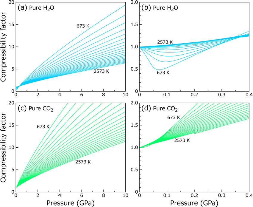
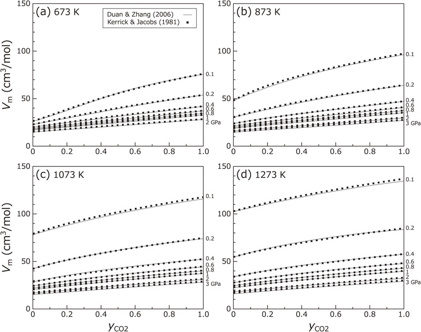
Figure 3 shows the molar volume (V_m) of the fluid as a function of fluid composition ($y_{\text{CO}_{2}}$). The molar volume is positively proportional to $y_{\text{CO}_{2}}$ because CO₂ is less compressible than H₂O. The V_m shows a convex upwards curve as a function of $y_{\text{CO}_{2}}$, indicating that the fluid mixing generates an excess of volume. The V_m values are consistent with those calculated from the equation of state by Kerrick and Jacobs (1981) within ∼ 5%.

Figure 3. The molar volume of H₂O-CO₂ mixture fluid at various pressures (0.1-3 GPa) and temperatures (673-1273 K). For comparison, the molar volumes calculated after Kerrick and Jacobs (1981) are shown as dots. These results are consistent within 5%.

Figures 4 and 5 show the activity-composition relation. At pressures of <1 GPa (Fig. 4), the activity-composition curves moderately positively deviate from the ideal mixing line. This trend is typical for most nonideal fluids and is consistent with previous studies (Flowers, 1979; Kerrick and Jacobs, 1981). However, at higher pressures (>3 GPa; Fig. 5), several curves show a complex, sometimes unusual shape, especially at high-pressure and low-temperature conditions. For example, at 873 K and pressure of >3 GPa, the activity curves do not show a simple monotonic increase or decrease but have maxima at $y_{\text{CO}_{2}}$ ∼ 0.05 (CO₂) and $y_{\text{CO}_{2}}$ ∼ 0.2-0.4 (H₂O). Similar peaks are observed at high pressures when the temperature is <1473 K. In addition, when the pressure is >5 GPa, curves for H₂O activity often deviate below the ideal mixing line at $y_{\text{CO}_{2}}$ ∼ 0.1-0.3. Whether such a trend is real has not been examined experimentally. These apparently unrealistic curves may be the result of inadequate calibration of parameters: although the number of simulation data is large (690 points), three fluid compositions ($y_{\text{CO}_{2}}$ = 0.25, 0.50, and 0.75) are only examined at each temperature and pressure (the interval of temperature and pressure was 50-100 K and 1 GPa, respectively). Therefore, users need to exercise caution when calculating the activity (and the partial fugacity coefficient) if the pressure is extremely high or if the temperature is low. Nevertheless, the equation of state seems to be valid enough for practical use if the pressure and temperature are appropriate for geologically realistic conditions. The equation of state seems to be safely used at most temperatures if the pressure is <3 GPa. For higher pressure conditions, the equation seems valid if the pressure-temperature conditions are on the typical geotherm.

Figure 4. Activity-composition diagrams for CO₂ (green) and H₂O (blue) at various temperatures (673-2573 K) and pressures (0.1, 0.3, 0.5, 0.7, and 0.9 GPa).

Figure 5. Activity-composition diagrams for CO₂ (green) and H₂O (blue) at various temperatures (673-2573 K) and pressures (1, 3, 5, 7, and 9 GPa).

A COMPUTER CODE FOR THE EQUATION OF STATE

It is desirable that a calculation code is provided so that readers can reproduce identical results without suffering from unnecessary errors. Such an effort has been made by, for example, Jacobs and Kerrick (1981), who provided Fortran and APL codes for the equation of state by Kerrick and Jacobs (1981). Here, a C-language code for the calculation of molar volume, compressibility factor, fugacity coefficient, and activity of the H₂O-CO₂ fluid is provided as Supplementary Material. A Windows executable program, which was produced by compiling the same code with MS Visual C++ .NET 2003 on Windows XP, is also provided for convenience. Readers may freely download these items from https://doi.org/10.2465/jmps.221224a and modify them for their purpose.

GEOLOGICAL IMPLICATIONS

The presented calculation showed that the mixing of H₂O and CO₂ occurs highly nonideally at crustal conditions: the molar volume of the mixed fluid is greater than the molar volume expected from ideal mixing (Fig. 3). If the volume is instead fixed, the pressure increases. This excess volume or pressure may exert a direct influence on geological phenomena such as CO₂ fluxing, in which a CO₂-rich fluid originated from deep-derived magma fluxes in an H₂O-rich shallow-stored magma (e.g., Yoshimura and Nakamura, 2011; van Hinsberg et al., 2016; Caricchi et al., 2018) and carbonic fluid metamorphism (metasomatism), in which a CO₂-rich fluid, possibly discharged from a magma, infiltrates into an H₂O-rich crustal rock (e.g., Frost and Frost, 1987; Newton, 1989, 1992). How the nonideal effects influence the phenomena is discussed here.

Figure 6 shows the molar volume of the H₂O-CO₂ fluid at 1123 K and 200 and 800 MPa. The pressure of 200 MPa is a typical condition for silicic magmas stored in the upper crust (e.g., Huber et al., 2019). If identical amounts of pure CO₂ fluid and pure H₂O fluid mix to produce the mixture fluid with $y_{\text{CO}_{2}}$ = 0.5 at this pressure, the molar volume of the mixed fluid is calculated to be 64.7 cm³/mol, which is ∼ 6.2% higher than the volume expected from the ideal mixing (60.9 cm³/mol). Therefore, if a fluid mixing phenomenon occurs in the crustal magma, a similar range of the volume increase is expected. This excess volume may exert a strong influence on the eruption dynamics because the increase in the fluid volume leads to an increase in magma buoyancy and may activate the convection of the magma chamber (e.g., Sparks et al., 1977). If the volume is instead fixed upon fluid mixing, then the fluid pressure increases to 221 MPa, which is ∼ 10% higher than before mixing. The pressure increase also influences the eruption dynamics, because the overpressure may act as a trigger for the eruption (e.g., Tait et al., 1989).

Figure 6. Molar volume of the H₂O-CO₂ fluid at 1123 K and 200 and 800 MPa. The volume of the mixture fluid (solid line) is larger than that expected from the ideal mixing (dashed line), indicating that a positive excesss volume is generated upon nonideal mixing. The molar volume at 221 and 892 MPa are also presented: these pressures were determined so that the molar volume of the fluid with $y_{\text{CO}_{2}}$ = 0.5 expected from the ideal mixing at 200 and 800 MPa is identical to the molar volume expected from the nonideal mixing.

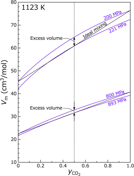
Figure 6 also shows the volume of the H₂O-CO₂ fluid at 800 MPa and 1123 K, a condition typical of the lower crust. If the fluid mixing associated with the carbonic fluid metamorphism occurs at this condition, the nonideal effect is still significant: if identical amounts of pure CO₂ fluid and pure H₂O mixes to produce the fluid of $y_{\text{CO}_{2}}$ = 0.5 at 800 MPa, an excess volume of ∼ 3.3% is expected (31.6 cm³/mol for the ideal mixing versus 32.9 cm³/mol for the nonideal mixing). If the volume is instead fixed, the excess pressure is ∼ 11% (the pressure after mixing is 892 MPa). These effects may promote metamorphism because the porosity increase enlarges the fluid pathways, while the pressure increase drives further fluid infiltration.

SUMMARY

The present study reviewed the equation of state for H₂O-CO₂ binary mixture fluid developed by Duan and Zhang (2006). The calculation procesure for the equation was presented. Also, a correct equation for the partial fugacity coefficient of the mixture fluid [Eq. (12)], which has been erroneously presented in previous studies, was provided. For most geologically realistic pressure-temperature conditions, molar volume, fugacity, and activity are well calculated with the equation. However, when the pressure is high and the temperature is low, caution should be used because the activity (the partial fugacity coefficient) seems to be unrealistic. Application to geological situations suggested that the excess volume generation or the pressure increase, which occur when a H₂O-rich fluid and a CO₂-rich fluid mix nonideally, may play an important role in volcanic eruption and metamorphism.

ACKNOWLEDGMENTS

I thank two anonymous reviewers and Editor Tetsu Kogiso for constructive comments. This study was supported by JSPS KAKENHI Grant Number JP20H01989.

SUPPLEMENTARY MATERIALS

Supplementary code and executable file are available online from https://doi.org/10.2465/jmps.221224a.

REFERENCES

• Albarède, F. (1995) Introduction to geochemical modeling. pp. 543, Cambridge University Press, Cambridge.
•  Anderko,  A. and  Pitzer,  K.S. (1991) Equation of state for pure fluids and mixtures based on a truncated virial expansion. AIChE Journal, 37, 1379-1391.
• Anderson, G. (2005) Thermodyanamics of natural systems. pp. 648, Cambridge University Press, Cambridge.
• Atkins, P. and de Paula, J. (2006) Physical chemistry, 8th edition, pp. 1067, Oxford University Press, Oxford.
•  Benedict,  M.,  Webb,  G.B. and  Rubin,  L.C. (1940) An empirical equation for thermodynamic properties of light hydrocarbons and their mixtures. I. Methane, ethane, propane and n-butane. The Journal of Chemical Physics, 8, 334-345.
•  Caricchi,  L.,  Shldrake,  T.E. and  Blundy,  J. (2018) Modulation of magmatic processes by CO₂ flushing. Earth and Planetary Sicnece Letters, 497, 160-171.
•  Duan,  X. (2014) A general model for predicting the solubility behavior of H₂O-CO₂ fluids in silicate melts over a wide range of pressure, temperature and compositions. Geochimica et Cosmochimica Acta, 125, 528-609.
•  Duan,  Z.,  Møller,  N. and  Weare,  J.H. (1992a) An equation of state for the CH₄-CO₂-H₂O system: I. Pure systems from 0 to 1000 °C and 0 to 8000 bar. Geochimica et Cosmochimica Acta, 56, 2605-2617.
•  Duan,  Z.,  Møller,  N. and  Weare,  J.H. (1992b) An equation of state for the CH₄-CO₂-H₂O system: II. Mixtures from 50 to 1000 °C and 0 to 1000 bar. Geochimica et Cosmochimica Acta, 56, 2619-2631.
•  Duan,  Z.,  Møller,  N. and  Weare,  J.H. (1992c) Molecular dynamics simulation of PVT properties of geological fluids and a general equation of state of nonpolar and weakly polar gases up to 2000 K and 20,000 bar. Geochimica et Cosmochimica Acta, 56, 3839-3845.
•  Duan,  Z.,  Møller,  N. and  Weare,  J.H. (1995) Molecular dynamics equation of state for nonpolar geochemical fluids. Geochimica et Cosmochimica Acta, 59, 1533-1538.
•  Duan,  Z.,  Møller,  N. and  Weare,  J.H. (1996) A general equation of state for supercritical fluid mixtures and molecular dynamics simulation of mixture PVTX properties. Geochimica et Cosmochimica Acta, 60, 1209-1216.
•  Duan,  Z. and  Zhang,  Z. (2006) Equation of state of the H₂O, CO₂, and H₂O-CO₂ systems up to 10 GPa and 2573.15 K: Molecular dynamics simulations with ab initio potential surface. Geochimica et Cosmochimica Acta, 70, 2311-2324.
•  Ferry,  J.M. and  Baumgartner,  L. (1987) Thermodynamic models of molecular fluids at the elevated pressures and temperatures of crustal metamorphism. Reviews in Mineralogy, 17, 323-365.
•  Flowers,  G.C. (1979) Correction of Holloway’s (1977) adaption of the modified Redlich-Kwong equation of state for calculation of the fugacities of molecular species in supercritical fluids of geologic interest. Contributions to Mineralogy and Petrology, 69, 315-318.
•  Frost,  B.R. and  Frost,  C.D. (1987) CO₂, melts and granulite metamorphism. Nature, 327, 503-506.
•  Ghiorso,  M.S. and  Gualda,  G.A.R. (2015) An H₂O-CO₂ mixed fluid saturation model compatible with rhyolite-MELTS. Contributions to Mineralogy and Petrology, 169, 53.
•  Gottschalk,  M. (2007) Equation of state for complex fluids. Reviews in Mineralogy and Geochemistry, 65, 49-97.
• Holloway, J.R. (1977) Fugacity and Activity of Molecular Species in Supercritical Fluids. In Thermodynamics in Geology (Fraser, D.G. Ed.). pp. 424, NATO Advanced Study Institutes Series, 30, Springer Netherlands, Dordrecht, 161-181.
•  Holloway,  J.R. (1987) Igneous fluids. Reviews in Mineralogy, 17, 211-233.
•  Huber,  C.,  Townsend,  M.,  Degruyter,  W. and  Bachmann,  O. (2019) Optimal depth of subvolcanic magma chamber growth controlled by volatiles ad crust rheology. Nature Geosciences, 12, 762-768.
•  Jacobs,  G.K. and  Kerrick,  D.M. (1981) APL and FORTRAN programs for a new equation of state for H₂O, CO₂, and their mixtures at supercritical conditions. Computer & Geosciences, 7, 131-143.
•  Kerrick,  D.M. and  Jacobs,  G.K. (1981) A modified Redlich-Kwong equation for H₂O, CO₂, and H₂O-CO₂ mixtures at elevated pressures and temperatures. American Journal of Science, 281, 735-767.
•  Lee,  B.I. and  Kesler,  M.G. (1975) A generalized thermodynamic correlation based on three-parameter corresponding states. AIChE Journal, 21, 510-527.
• Mitchell, M., Muftakhidinov, B. and Winchen, T. (2008) Engauge Digitizer Software. doi:10.5281/zenodo.3941227.
•  Newton,  R.C. (1989) Metamorphic fluids in the deep crust. Annual Review of Earth and Planetary Sciences, 17, 385-412.
•  Newton,  R.C. (1992) Charnockitic alteration: evidence for CO₂ infiltration in granulite facies metamorphism. Journal of Metamorphic Geology, 10, 383-400.
•  Nieva,  D. and  Barragán,  R.M. (2003) HCO-TERNARY: A FORTRAN code for calculating P-V-T-X properties and liquid vapor equilibria of fluids in the system H₂O-CO₂-CH₄. Computer & Geosciences, 29, 469-485.
• Nordstrom, D.K. and Munoz, J.L. (1994) Geochemical thermodynamics, second edition. pp. 493, The Blackburn Press, New Jersey.
•  Pitzer,  K. and  Curl,  R.F.Jr. (1957) The volumetric and thermodynamic properties of fluids III. Empirical equation for the second virial coefficient. Journal of the American Chemical Society, 79, 2369-2370.
• Poling, B.E., Prausnitz, J.M. and O’connell, J.P. (2001) The properties of gases and liquids, fifth edition, pp. 768, McGraw-Hill.
• Prausnitz, J.M., Lichtenthaler, R.N. and de Azevedo, E.G. (1999) Molecular thermodynamics of fluid-phase equilibria, third edition. pp. 860, Prentice Hall PTR, New Jersey.
•  Shibue,  Y. (1995) Redlich-Kwong equation of state: An equation of state for fluid. Shigen-Chishitsu, 45, 121-127.
•  Sparks,  S.R.J.,  Sigurdsson,  H. and  Wilson,  L. (1977) Magma mixing: a mechanism for triggering acid explosive eruptions. Nature, 267, 315-317.
•  Tait,  S.,  Jaupart,  C. and  Vergniolle,  S. (1989) Pressure, gas constant and eruptioin periodicity of a shallow crystallising magma chamber. Earth and Planetary Science Letters, 92, 107-123.
•  van Hinsberg,  V.J.,  Berlo,  K.,  Migdisov,  A.A. and  Williams-Jones,  A.E. (2016) CO₂-fluxing collapses metal mobility in magmatic vapour. Geochemical Perspectives Letters, 2, 169-177.
• Walas, S.M. (1985) Phase equilibria in chemical engineering. pp. 671, Butterworth Publishers, Massachusetts.
•  Yoshimura,  S. (2023) Carbon dioxide and water in the crust. Part 2: Solubility in silicate melts. Journal of Mineralogical and Petrological Sciences, 118, 023.
•  Yoshimura,  S. and  Nakamura,  M. (2011) Carbon dioxide transport in crustal magmatic systems. Earth and Planetary Science Letters, 307, 470-478.

APPENDIX A: THE ORIGINAL LEE-KESLER EQUATION

The original Lee-Kesler equation (Lee and Kesler, 1975) is briefly reviewed here. The Lee-Kesler equation was developed based on the formulation of the BWR equation (Benedict et al., 1940) and the concept of acentric factor by Pitzer and Curl (1957). The equation is the corresponding-state equation and applies to many fluids if their critical pressure, critical temperature, and acentric factor are identified. The acentric factor is the measure of deviation of the intermolecular potential from that of a ‘simple’ fluid, which is composed of a spherical, nonpolar molecule such as methane, argon, and krypton (Pitzer and Curl, 1957). In the Lee-Kesler formulation the compressibility factor of the fluid (Z) is given as:

  

\begin{equation} Z = Z^{(0)} + \frac{\omega}{\omega^{(r)}}(Z^{(r)} - Z^{(0)}) \end{equation} (A1),

where Z⁽⁰⁾ is the compressibility factor of a simple fluid and Z^(r) is the compressibility factor for a ‘reference’ fluid, the representative of which is n-octane, the heaviest hydrocarbon for which there are extensive data. ω is the acentric factor for the fluid of interest and ω^(r) is the acentric factor for the reference fluid (ω^(r) is fixed to 0.3978, the value for n-octane). Eq. (A1) therefore means that Z of the fluid is provided as the sum of Z of the simple fluid and the deviation from the simple fluid. Z⁽⁰⁾ and Z^(r) are calculated separately with the following equation (so-called Lee-Kesler equation):

  

\begin{align} Z &= \frac{PV_{\text{m}}}{RT} = 1 + \frac{BV_{\text{c}}}{V_{\text{m}}} + \frac{CV_{\text{c}}^{2}}{V_{\text{m}}^{2}} + \frac{EV_{\text{c}}^{5}}{V_{\text{m}}^{5}} + \frac{FV_{\text{c}}^{2}}{V_{\text{m}}^{2}}\left(\beta + \frac{\gamma V_{\text{c}}^{2}}{V_{\text{m}}^{2}}\right)\exp\left(-\frac{\gamma V_{\text{c}}^{2}}{V_{\text{m}}^{2}}\right) \end{align} (A2),

where parameters are provided as:

  

\begin{equation} B = b_{1} - b_{2}\left(\frac{T_{\text{c}}}{T}\right) - b_{3}\left(\frac{T_{\text{c}}}{T}\right)^{2} {}- b_{4}\left(\frac{T_{\text{c}}}{T}\right)^{3} \end{equation} (A3),

  

\begin{equation} C = c_{1} - c_{2}\left(\frac{T_{\text{c}}}{T}\right) + c_{3}\left(\frac{T_{\text{c}}}{T}\right)^{3} \end{equation} (A4),

  

\begin{equation} E = e_{1} + e_{2}\left(\frac{T_{\text{c}}}{T}\right) \end{equation} (A5),

and

  

\begin{equation} F = c_{4}\left(\frac{T_{\text{c}}}{T}\right)^{3} \end{equation} (A6).

Here, parameter values used in Eq. (A2)-(A6) are listed in Table A1. Equation (A2) is similar to Eq. (1) of the main text, but the fourth-order term is not used here.

The acentric factor in Eq. (A1) is defined as:

  

\begin{equation} \omega = -\log_{10}\left(\frac{P_{T_{\text{r}} = 0.7}^{\text{sat}}}{P_{\text{c}}}\right) - 1 \end{equation} (A7),

where $P_{T_{\text{r}} = 0.7}^{\text{sat}}$ represents the saturation vapour pressure of the volatile at the reduced temperature $(T_{\text{r}} = \frac{T}{T_{\text{c}}})$ of 0.7. The value of ω is dependent on the substance, and it is ∼ 0 when the molecule is spherical (simple fluid), while it is a greater value when the molecule is nonspherical and polarized. The ω values are listed in literature such as Appendix of Poling et al. (2001).

The calculation is performed as follows: First, calculate Z⁽⁰⁾ and Z^(r) separately according to Eq. (A2)-(A6), values in Table A1, and P_c and T_c values of the fluid of interest. Second, find ω of the fluid from the literature or calculate ω based on experimental data and Eq. (A7). Finally, input all these values in Eq. (A1) to obtain Z of the fluid.

Table A1. Values for parameters in the original Lee-Kesler equation of state

Parameters	Simple fluids	Reference fluids
b1	0.1181193	0.2026579
b2	0.265728	0.331511
b3	0.154790	0.027655
b4	0.030323	0.203488
c1	0.0236744	0.0313385
c2	0.0186984	0.0503618
c3	0.0	0.016901
c4	0.042724	0.041577
e1	1.55488 × 10−5	4.8736 × 10−5
e2	6.23689 × 10−5	7.40336 × 10−6
β	0.65392	1.226
γ	0.060167	0.03754

Reproduced from Lee and Kesler (1975).