Carbon dioxide and water in the crust. Part 2: Solubility in silicate melts

Abstract

The solubility of H₂O and CO₂ in silicate melts is crucial in understanding the geological phenomena occurring in a fluid-melt system. Although several recent solubility models are used in petrological studies, the model of Duan (2014) has rarely been used and has been evaluated less thoroughly, despite its potentially high applicability, mainly because calculation software is unavailable. This paper reviews the Duan (2014) solubility model and its calculation procedure for H₂O-CO₂ solubility. It was found that the Duan (2014) model uses a special protocol to calculate the fluid partial fugacity coefficient, for which no explanation is given in the original paper, thereby limiting the general use of the model. Therefore, I present an appropriate calculation procedure and provide a C-language code for convenience. The predictability of the model was evaluated by comparison with experimental solubility data. It was shown that the Duan (2014) model reproduces well the data for rhyolitic melts, whereas predictability is somewhat weak for other melts, including dacitic, andesitic, and basaltic melts. Caution is thus required when applying the Duan (2014) model to SiO₂-poor melts.

INTRODUCTION

Volatiles dissolved in silicate melt control phase relations and physicochemical properties of the melt. When the volatile content exceeds the solubility limit, fluid exsolution occurs, causing dramatic changes in bulk density, bulk viscosity, and the elemental partitioning. Volatile solubility is therefore crucial in understanding the fluid-involved geological phenomena. Because H₂O and CO₂ are the major volatiles, many experimental studies have investigated the solubility of pure H₂O and CO₂ and H₂O-CO₂ mixture (see Holloway and Blank, 1994; Moore, 2008; Baker and Alletti, 2012, for a comprehensive review). Solubility models were constructed based on experimental data and thermodynamic or empirical equations. Models with high predictability and wide applicability are required to promote our understanding of geological phenomena.

For the practical use of a solubility model in petrological studies, accessibility and usability are also important factors. In this regard, the solubility model developed by Newman and Lowenstern (2002) has received great attention because the authors developed a user-friendly MS Excel program (VolatileCalc), through which the solubility of H₂O and CO₂ for both rhyolitic and basaltic melts could easily be computed. Papale (1997, 1999) and Papale et al. (2006) pioneered general thermodynamic models that predict H₂O-CO₂ solubility in silicate melts with arbitrary compositions, providing a new tool to study fluid-melt equilibrium in varieties of natural magmas. Ghiorso and Gualda (2015) then developed a solubility model applicable to various silicate compositions and a wide pressure-temperature range (MagmaSat). This model is compatible with Rhyolite-MELTS (Gualda et al., 2012) and is becoming increasingly popular because the calculation can be performed relatively easily through a web application or software package. More recently, Iacovino et al. (2021) and Wieser et al. (2022) developed a new type of solubility calculation package (VESIcal), through which H₂O-CO₂ fluid saturation conditions can be computed based on seven solubility models, namely Ghiorso and Gualda (2015) (MagmaSat), Dixon (1997), Moore et al. (1998), Liu et al. (2005), Iacono-Marziano et al. (2012), Shishkina et al. (2014), and Allison et al. (2019). VESIcal enables not only solubility calculation but also a comparison of the models, allowing a less biased interpretation of the fluid-melt equilibrium state.

One solubility model that has both wide applicability and clear equation sets, but has not been thoroughly examined, is the model of Duan (2014). This solubility model is constructed on a thermodynamic basis and is applicable to wide pressure-temperature conditions (up to 3 GPa and 933-2003 K) and varieties of melt compositions from ultramafic to rhyolitic (granitic) melts. However, despite its potentially high applicability, the Duan (2014) model has rarely been used, and it was also excluded from recent reviews because the software for the solubility calculation is not available (Iacovino et al., 2021; Wieser et al., 2022). Previously, a Windows executable file and a web application were provided on Duan’s personal website, but these are no longer available. In addition, calculation protocols for the partial fugacity coefficient, which is required for solubility calculation and is computed through the equation of state by Duan and Zhang (2006), seem to have been modified from those of the original paper without providing any clear explanation, limiting the general use of the model in the petrological community. This paper reviews the Duan (2014) solubility model and show the modified calculation protocol for the partial fugacity coefficient. A C-language code and an executable program for solubility calculation are also provided so that readers will be able to freely use or implement the model in their work. The suitability of the Duan (2014) model is evaluated by comparison with experimental data. The model is also compared with MagmaSat (Ghiorso and Gualda, 2015) to illustrate their differences in predictability.

H₂O AND CO₂ DISSOLUTION SPECIES IN SILICATE MELTS

Before focusing on the Duan (2014) solubility model, dissolution species of H₂O and CO₂ in silicate melts are briefly overviewed (see, e.g., Blank and Brooker, 1994; McMillan, 1994; Zhang, 1999; Zhang et al., 2007, for a comprehensive review). Infrared spectroscopy revealed that H₂O dissolves in silicate melts as both hydroxyl groups (OH) and H₂O molecules (H₂O_mol) through the fluid-melt reaction (1a) and the homogeneous dissociation reaction (1b):

  

\begin{equation} \text{H$_{2}$O (fluid)} \leftrightarrow \text{H$_{2}$O$_{\text{mol}}$ (melt)} \end{equation} (1a)

and

  

\begin{equation} \text{H$_{2}$O$_{\text{mol}}$ (melt)} + \text{O (melt)} \leftrightarrow \text{2OH (melt)} \end{equation} (1b),

where O (melt) is the bridging oxygen (and a small amount of free oxygen) (Zhang et al., 2007). For a given melt, the ratio of OH and H₂O_mol changes as a function of the total H₂O (OH + H₂O_mol) content: as the total H₂O content increases, the ratio of OH/H₂O_mol decreases (e.g., Zhang, 1999). Therefore, a water-poorer melt has a higher OH/H₂O_mol ratio. The OH/H₂O_mol ratio also increases with increasing temperature (e.g., Ihinger et al., 1999). In the present study, the term H₂O content is used in a generic sense for the total H₂O because the Duan (2014) solubility model only considers the total H₂O content and does not take into account the speciation reaction.

CO₂ dissolves in silicate melt as CO₂ molecules (CO_2mol) and/or carbonate ions (CO₃²⁻) through the following reaction:

  

\begin{equation} \text{CO$_{2}$ (fluid)} \leftrightarrow \text{CO$_{2\,\text{mol}}$ (melt)} \end{equation} (2a)

and

  

\begin{equation} \text{CO$_{2\,\text{mol}}$ (melt)} + \text{O$^{2-}$ (melt)} \leftrightarrow \text{CO$_{3}^{2-}$ (melt)} \end{equation} (2b),

where O²⁻ denotes the non-bridging oxygen (Ni and Keppler, 2013). Therefore, which of the species (CO_2mol or CO₃²⁻) is dominant or exclusive is a function of the degree of polymerization of the melt, which is strongly dependent on melt composition and water content (e.g., Konschak and Keppler, 2014). In general, rhyolitic melts contain CO_2mol as the single species, basaltic melt only contains CO₃²⁻, and intermediate melts contain both species. Note however that the presence of CO₃²⁻ in hydrous high-SiO₂ rhyolitic melts was reported by recent studies (Moore et al., 2008; Yoshimura et al., 2017). Hereafter, the term CO₂ content is used for the content of all CO₂ species dissolved in the melt irrespective of the CO₃²⁻/CO_2mol ratio. The Duan (2014) model only predicts the total CO₂ content for silicate melt and does not deal with the speciation reaction.

THERMODYNAMICS OF VOLATILE SOLUBILITY IN SILICATE MELTS

The Duan (2014) solubility model is constructed on a thermodynamic basis. Consider a situation where a H₂O-CO₂ binary mixture fluid with a H₂O molar fraction of y₁ and a CO₂ molar fraction of y₂ (thus, y₁ + y₂ = 1) coexists with a silicate melt at constant pressure and temperature. At the fluid-melt equilibrium state, the chemical potential of the volatile component i (H₂O or CO₂) in the fluid, $\mu_{i}^{\text{fluid}}$, is identical to that of the melt, $\mu_{i}^{\text{melt}}$:

  

\begin{equation} \mu_{i}^{\text{fluid}} = \mu_{i}^{\text{melt}} \end{equation} (3).

$\mu_{i}^{\text{fluid}}$ is expressed as:

  

\begin{equation} \mu_{i}^{\text{fluid}} = \mu_{i}^{\text{fluid,ref}} + RT\ln \frac{f_{i}}{f_{i}^{\text{ref}}} \end{equation} (4),

where $\mu_{i}^{\text{fluid},\text{ref}}$ is the chemical potential of volatile component i at a reference state, R is the gas constant (0.083 kbar cm³ mol⁻¹ K⁻¹), T is the temperature (K), f_i is the fugacity of volatile component i in the fluid (kbar), and $f_{i}^{\text{ref}}$ is the fugacity of volatile component i at the reference state. f_i is written as:

  

\begin{equation} f_{i} = \phi_{i}P_{i} = \phi_{i}y_{i}P \end{equation} (5),

where ϕ_i is the partial fugacity coefficient of volatile component i, P_i is the partial pressure of volatile component (kbar), and P denotes the total pressure (kbar). If the pressure of the reference state is set to unity, Eq. (4) is simplified to:

  

\begin{equation} \mu_{i}^{\text{fluid}} = \mu_{i}^{\text{fluid,ref}} + RT\ln(\phi_{i}y_{i}P) \end{equation} (6).

For the melt, the chemical potential of volatile component i dissolved in the melt is expressed as:

  

\begin{equation} \mu_{i}^{\text{melt}} = \mu_{i}^{\text{melt,ref}} + RT\ln a_{i}^{\text{melt}} \end{equation} (7),

where $\mu_{i}^{\text{melt},\text{ref}}$ is the chemical potential of volatile component i in the melt at the reference state. $a_{i}^{\text{melt}}$ represents the activity of volatile component i in the melt and is expressed as:

  

\begin{equation} a_{i}^{\text{melt}} = \gamma_{i}^{\text{melt}}\,x_{i} \end{equation} (8),

where $\gamma_{i}^{\text{melt}}$ is the activity coefficient and x_i is the molar fraction of volatile component i. In the Duan (2014) model, x_i is defined as the molar fraction on a single oxygen basis, that is, the molar fraction of volatile i calculated on the assumption that the molar mass of volatile-free melt is the mass of melt per mole of oxygen [see Eqs. (17a), (17b), and (18)].

Based on the presented equations, Eq. (3) becomes:

  

\begin{equation} \mu_{i}^{\text{fluid,ref}} + RT\ln(\phi_{i}y_{i}P) = \mu_{i}^{\text{melt,ref}} + RT\ln (\gamma_{i}^{\text{melt}}x_{i}) \end{equation} (9).

Rearranging Eq. (9), the following equation is obtained:

  

\begin{equation} RT\ln \left(\frac{\phi_{i}y_{i}P}{\gamma_{i}^{\text{melt}}\,x_{i}}\right) = \mu_{i}^{\text{melt,ref}} - \mu_{i}^{\text{fluid,ref}} \end{equation} (10).

Eq. (10) is the basic solubility equation for the Duan (2014) model. On the left-hand side, ϕ_i can be calculated from the equation of state. Here, the equation of state by Duan and Zhang (2006) is exclusively used in the Duan (2014) model (see the next section). $\gamma_{i}^{\text{melt}}$ is calculated from the modified version of the Margules-type regular solution model as shown later [see Eqs. (15) and (16)]. For the right-hand side, Duan (2014) assumed $\mu_{i}^{\text{fluid},\text{ref}}$ to be 0 and described $\mu_{i}^{\text{melt},\text{ref}}$ as an empirical function:

  

\begin{align} \mu_{i}^{\text{melt,ref}} &= c_{1} + c_{2}T + c_{3}P^{2} \\&\quad+ \frac{c_{4}}{T} + c_{5}\ln T + \frac{c_{6}P^{2}}{T} + c_{7}P \end{align} (11),

where c₁-c₇ are constant values for H₂O and CO₂ (Table 1). Therefore, the solubility of volatile i (i.e., x_i) is obtained by solving Eq. (10) under a given pressure, temperature and composition of coexisting fluid (y_i). Note that $\mu_{i}^{\text{melt},\text{ref}}$ was denoted as ‘$\mathit{Par}\,(T, P)$’ in the original paper [Eq. (21) in Duan (2014)].

Table 1. Parameters for Eq. (11)

Parameters	H2O	CO2
c1	162.95	111414.92
c2	0.34	6.06
c3	0.61	−0.53
c4	0	−10873021.59
c5	0	−15390.5
c6	0	986.72
c7	0	25.03

Reproduced from Table 4 of Duan (2014).

It should be noted that throughout the calculation of the Duan (2014) model, several different values are used for the gas constant R because the units of pressure and fluid volume differ according to the calculation section. In Eqs. (4)-(10), the value of R is 0.083 kbar cm³ K⁻¹ mol⁻¹, whereas it is 83.14467 bar cm³ K⁻¹ mol⁻¹ when calculating the partial fugacity coefficient through the equation of state by Duan and Zhang (2006). When calculating the activity coefficient of melt in Eqs. (15) and (16) (see later section), R is 8.3 J K⁻¹ mol⁻¹. The values of constants used in the present study are summarized in Supplementary Document (available online from https://doi.org/10.2465/jmps.221224b).

CALCULATION OF THE PARTIAL FUGACITY COEFFICIENT OF COEXISTING FLUID

The Duan (2014) solubility model exclusively uses the equation of state developed by Duan and Zhang (2006) to calculate the partial fugacity coefficient (ϕ_i) of the coexisting fluid. Because the details of the equation of state were reviewed in Part 1 (Yoshimura, 2023), only brief descriptions are provided here.

The Duan and Zhang (2006) equation of state is given as:

  

\begin{align} Z = \frac{PV_{\text{m}}}{RT} &= 1 + \frac{BV_{c}}{V_{\text{m}}} + \frac{CV_{\text{c}}^{2}}{V_{\text{m}}^{2}} + \frac{DV_{\text{c}}^{4}}{V_{\text{m}}^{4}} + \frac{EV_{\text{c}}^{5}}{V_{\text{m}}^{5}} \\&\quad+ \frac{FV_{\text{c}}^{2}}{V_{\text{m}}^{2}}\left(\beta + \frac{\gamma V_{\text{c}}^{2}}{V_{\text{m}}^{2}}\right)\exp\left(-\frac{\gamma V_{\text{c}}^{2}}{V_{\text{m}}^{2}}\right) \end{align} (12),

where Z is the compressibility factor (a dimensionless number), P is the pressure (bar), V_m is the molar volume of the fluid (cm³ mol⁻¹), R is the gas constant (83.14467 bar cm³ K⁻¹ mol⁻¹), and T is the temperature (K). The parameters B, C, D, E, F, β, and γ are temperature-dependent values for H₂O and CO₂, and two sets of values are prepared: when the pressure is ≤0.2 GPa, the low-pressure values are used, whereas when the pressure is 0.2-10 GPa, the high-pressure values are used (see Supplementary Document). V_c is the molar volume of the fluid at the critical temperature and pressure for pure H₂O or CO₂ fluid. When the fluid is a mixture of H₂O and CO₂, the terms BV_c, $CV_{\text{c}}^{2}$, … are calculated based on mixing rules (see Supplementary Document).

The partial fugacity coefficient of component i in the fluid, ϕ_i, is given as:

  

\begin{align} &\ln \phi_{i} \\ & \quad = -\ln Z + \frac{(BV_{\text{c}})_{i}{'}}{V_{\text{m}}} + \frac{(CV_{\text{c}}^{2})_{i}{'}}{2V_{\text{m}}^{2}} + \frac{(DV_{\text{c}}^{4})_{i}{'}}{4V_{\text{m}}^{4}} + \frac{(EV_{\text{c}}^{5})_{i}{'}}{5V_{\text{m}}^{5}} \\ & \qquad + \frac{(FV_{\text{c}}^{2})_{i}{'}\beta + \beta_{i}{'}FV_{\text{c}}^{2}}{2\gamma V_{\text{c}}^{2}}\left[1 - \exp\left(-\frac{\gamma V_{\text{c}}^{2}}{V_{\text{m}}^{2}}\right)\right] \\ & \qquad + {\frac{(FV_{\text{c}}^{2})_{i}{'}\gamma V_{\text{c}}^{2} + (\gamma V_{\text{c}}^{2})_{i}{'}FV_{\text{c}}^{2} - FV_{\text{c}}^{2}\beta[(\gamma V_{\text{c}}^{2})_{i}{'} - \gamma V_{\text{c}}^{2}]}{2(\gamma V_{\text{c}}^{2})^{2}}}\\ & \qquad \times\left[1 - \left(\frac{\gamma V_{\text{c}}^{2}}{V_{\text{m}}^{2}} + 1\right)\exp\left(-\frac{\gamma V_{\text{c}}^{2}}{V_{\text{m}}^{2}}\right)\right] \\ & \qquad -\frac{[(\gamma V_{\text{c}}^{2})_{i}{'} - \gamma V_{\text{c}}^{2} ]FV_{\text{c}}^{2}}{2(\gamma V_{\text{c}}^{2})^{2}}\\ & \qquad \times\left[2 - \left(\frac{(\gamma V_{\text{c}}^{2})^{2}}{V_{\text{m}}^{4}} + \frac{2\gamma V_{\text{c}}^{2}}{V_{\text{m}}^{2}} + 2\right)\exp\left(-\frac{\gamma V_{\text{c}}^{2}}{V_{\text{m}}^{2}}\right)\right] \end{align} (13)

where $(BV_{\text{c}})_{i}{'}$, $(CV_{\text{c}}^{2})_{i}{'}$, … are calculated according to the equations given in Supplementary Document. Note that Eq. (13) has long been erroneously presented in previous studies including Duan and Zhang (2006) (see Part 1 for the detail; Yoshimura, 2023).

It was found that the calculation of the partial fugacity coefficient is problematic in the Duan (2014) model. Duan and Zhang (2006) instructed that the partial fugacity coefficient should be calculated in the following manner: when the pressure is <0.2 GPa, ϕ_i is calculated directly from Eq. (13) with low-pressure values, whereas when the pressure is >0.2 GPa, ϕ_i is calculated as:

  

\begin{equation} \ln \phi_{i} = \ln \phi_{i}^{\text{high},P} - \ln \phi_{i}^{\text{high}, 0.2\,\text{GPa}} + \ln \phi_{i}^{\text{low}, 0.2\,\text{GPa}} \end{equation} (14),

where $\phi_{i}^{\text{high},P}$ is the partial fugacity coefficient calculated from Eq. (13) with the high-pressure variables and the given pressure, $\phi_{i}^{\text{high}, 0.2\,\text{GPa}}$ is the partial fugacity coefficient calculated from Eq. (13) with the high-pressure variables and a pressure of 0.2 GPa, and $\phi_{i}^{\text{low}, 0.2\,\text{GPa}}$ is the partial fugacity coefficient calculated from Eq. (13) with the low-pressure variables and a pressure of 0.2 GPa. Here, 0.2 GPa is the pressure at which parameter values switch. If this protocol is used, however, the calculated solubility is much higher than that calculated using the Windows executable file previously provided on Duan’s website (Fig. 1).

Figure 1. Comparison between H₂O-CO₂ solubility calculated from equations presented in this study and that calculated with the Windows executable file previously provided on Duan’s website (now unavailable). (a) Rhyolitic melt [EDF of Tamic et al. (2001)] at 1273.15 K and (b) basaltic melt [TT152-51-3 of Dixon et al. (1995)] at 1375.15 K. Melt compositions of EDF and TT152-51-3 are summarized in Supplementary Document. Solubility calculated in the present study without using Eq. (14) agrees well with Duan’s solubility within 2.5%, whereas that calculated using Eq. (14) is significantly higher than that using Duan’s solubility.

At pressures >0.2 GPa this discrepancy was always observed irrespective of temperature, pressure, and melt composition. In contrast, at pressures <0.2 GPa no significant discrepancy was observed. After trial and error, it was found that, if ϕ_i is calculated simply from Eq. (13) without using Eq. (14), even if P > 0.2 GPa, then the solubility results agree well with the values obtained by using the executable file of Duan (2014) (within a relative deviation of <2.5%) (Fig. 1). Therefore, it appears that Duan (2014) established the solubility model without following the official protocol of Duan and Zhang (2006). In the present study, Eq. (13) is only used irrespective of the pressure condition, and Eq. (14) is temporarily abandoned.

CALCULATION OF ACTIVITY COEFFICIENTS IN MELT

In the Duan (2014) solubility model, the activity coefficient for H₂O ($\gamma_{\text{H${_{2}}$O}}$) and CO₂ ($\gamma_{\text{CO}_{2}}$) of silicate melt is calculated based on a modified Margules-type regular solution model:

  

\begin{align} &RT\ln \gamma_{\text{H${_{2}}$O}} \\ & \quad = (1 - x_{\text{H${_{2}}$O}}) x_{\text{CO}_{2}}w_{\text{H${_{2}}$OCO${_{2}}$}} \\ & \qquad + (1 - x_{\text{H${_{2}}$O}})(1 - x_{\text{H${_{2}}$O}} - x_{\text{CO}_{2}})\sum_{j(\ne \text{CO}_{2}) = 1}^{n}(x_{j}w_{\text{H${_{2}}$O}j}) \\ & \qquad - x_{\text{CO}_{2}}(1 - x_{\text{CO}_{2}} - x_{\text{H${_{2}}$O}})\sum_{j(\ne \text{H${_{2}}$O}) = 1}^{n}(x_{j}w_{\text{CO}_{2}j}) \\ & \qquad - (1 - x_{\text{CO}_{2}} - x_{\text{H${_{2}}$O}})^{2}\\ & \qquad \times\sum_{j(\ne \text{CO}_{2}, \text{H${_{2}}$O}) = 1}^{n - 1} \left[\sum_{k(\ne \text{CO}_{2}, \text{H${_{2}}$O}) = j + 1}^{n}(x_{j}x_{k}w_{jk})\right] \end{align} (15),

and

  

\begin{align} &RT\ln \gamma_{\text{CO}_{2}} \\ & \quad= (1 - x_{\text{CO}_{2}}) x_{\text{H${_{2}}$O}}w_{\text{CO}_{2}\text{H${_{2}}$O}} \\ & \qquad+ (1 - x_{\text{CO}_{2}})(1 - x_{\text{CO}_{2}} - x_{\text{H${_{2}}$O}})\sum_{j(\ne \text{H${_{2}}$O}) = 1}^{n}(x_{j}w_{\text{CO}_{2}j}) \\ & \qquad - x_{\text{H${_{2}}$O}}(1 - x_{\text{H${_{2}}$O}} - x_{\text{CO}_{2}})\sum_{j(\ne \text{CO}_{2}) = 1}^{n}(x_{j}w_{\text{H${_{2}}$O}j}) \\ & \qquad - (1 - x_{\text{CO}_{2}} - x_{\text{H${_{2}}$O}})^{2}\\ & \qquad\times\sum_{j(\ne \text{CO}_{2}, \text{H${_{2}}$O}) = 1}^{n-1} \left[\sum_{k(\ne \text{CO}_{2}, \text{H${_{2}}$O}) = j + 1}^{n}(x_{j}x_{k}w_{jk}) \right] \end{align} (16).

Here, the value of the gas constant R is 8.3 (J K⁻¹ mol⁻¹). $x_{\text{H${_{2}}$O}}$ and $x_{\text{CO}_{2}}$ are the molar fractions of H₂O and CO₂ on a single oxygen basis, respectively (Zhang, 1999):

  

\begin{equation} x_{\text{H${_{2}}$O}} = \frac{\cfrac{C_{\text{H${_{2}}$O}}}{M_{\text{H${_{2}}$O}}}}{\cfrac{C_{\text{H${_{2}}$O}}}{M_{\text{H${_{2}}$O}}} + \cfrac{C_{\text{CO}_{2}}}{M_{\text{CO}_{2}}} + \cfrac{1 - C_{\text{H${_{2}}$O}} - C_{\text{CO}_{2}}}{W}} \end{equation} (17a),

and

  

\begin{equation} x_{\text{CO}_{2}} = \frac{\cfrac{C_{\text{CO}_{2}}}{M_{\text{CO}_{2}}}}{\cfrac{C_{\text{H${_{2}}$O}}}{M_{\text{H${_{2}}$O}}} + \cfrac{C_{\text{CO}_{2}}}{M_{\text{CO}_{2}}} + \cfrac{1 - C_{\text{H${_{2}}$O}} - C_{\text{CO}_{2}}}{W}} \end{equation} (17b),

where $C_{\text{H${_{2}}$O}}$ and $C_{\text{CO}_{2}}$ are the weight fractions of H₂O and CO₂ in the melt, respectively (0 ≤ C_i ≤ 1). $M_{\text{H${_{2}}$O}}$ and $M_{\text{CO}_{2}}$ are the molar masses of H₂O (18.02 g mol⁻¹) and CO₂ (44.01 g mol⁻¹), respectively. W is the mass of volatile-free melt per mole of oxygen (g per 1 mol oxygen):

  

\begin{equation} W = \frac{\displaystyle\sum_{j(\ne \text{CO}_{2},\text{H${_{2}}$O}) = 1}^{n}C_{j}}{\displaystyle\sum_{j(\ne \text{CO}_{2},\text{H${_{2}}$O}) = 1}^{n}\left(\frac{C_{j}}{M_{j}} \times n_{j}^{\text{oxygen}}\right)} \times 100 \end{equation} (18),

where $n_{j}^{\text{oxygen}}$ is the number of oxygen atoms in a one-formula oxide component j (e.g., $n_{\text{Al${_{2}}$O${_{3}}$}}^{\text{oxygen}}$ = 3, $n_{\text{MgO}}^{\text{oxygen}}$ = 1). C_j and M_j represent the weight fraction (0 ≤ C_j ≤ 1) and molar mass (g mol⁻¹) of non-volatile oxide j, respectively. Values of M_j used in the present study are summarized in Supplementary Document.

In Eqs. (15) and (16), $x_{j(\ne \text{CO}_{2}, \text{H${_{2}}$O})}$ is the molar fraction of non-volatile oxide component j in the volatile-free melt:

  

\begin{equation} x_{j (\ne \text{CO}_{2}, \text{H${_{2}}$O})} = \frac{\cfrac{C_{j}}{M_{j}}}{\displaystyle\sum_{j (\ne \text{H${_{2}}$O}, \text{CO}_{2}) = 1}^{n}\frac{C_{j}}{M_{j}}} \end{equation} (19).

$w_{\text{H${_{2}}$O}j}$ and $w_{\text{CO}_{2}j}$ in Eqs. (15) and (16) are the interaction parameters between H₂O and non-volatile oxide component j and those between CO₂ and non-volatile oxide component j. Values of $w_{\text{H${_{2}}$O}j}$ and $w_{\text{CO}_{2}j}$ are provided in Table 2. w_jk is the interaction parameter between two non-volatile oxide components j and k, the values of which are taken from Ghiorso et al. (1983) (Table 3). Note that the unit of $w_{\text{H${_{2}}$O}j}$ and $w_{\text{CO}_{2}j}$ is J, whereas the unit of w_jk in Ghiorso et al. (1983) is cal. Therefore, the values of w_jk need to be multiplied by 4.2 J cal⁻¹ when input in Eqs. (15) and (16) (e.g., $w_{\text{SiO${_{2}}$-Al${_{2}}$O${_{3}}$}}$ = −78563.2 cal in Ghiorso et al. (1983) → −329965.44 J).

Table 2. Interaction parameters

j	wH2Oj (J)	wCO2j (J)
CO2 or H2O	0	0
SiO2	−41274	33754
TiO2	0	0
Al2O3	−347360	−190544
Fe2O3	−11701	−36074
FeO	−65722	−17398
MnO	0	0
MgO	−131718	−86063
CaO	−202184	−203394
Na2O	−266067	−298072
K2O	−308212	−663279

Reproduced from Table 4 of Duan (2014).

Table 3. Interaction parameters, w_jk (cal)

	SiO2	TiO2	Al2O3	Fe2O3	FeO	MnO	MgO	CaO	Na2O
SiO2
TiO2	−29364.5
Al2O3	−78563.2	−67349.7
Fe2O3	2637.93	−6821.82	1240.32
FeO	−9630.14	−4594.59	−59528.6	4524.46
MnO	5525.36	−2043.20	−1917.75	212.196	−703.34
MgO	−30353.6	12673.6	−48674.8	−1277.03	−57925.8	−2810.1
CaO	−64068.1	−102442	−98428.3	1519.81	−59355.5	699.123	−78924.5
Na2O	−73758.3	−101074	−135615	−3717.38	−36966.2	780.15	−92611.4	−62779.9
K2O	−87596.4	−40700.7	−175326	283.726	−84579.5	−60.7241	−45162.9	−27908	−18129.7

Values reproduced from Table A4-3 of Ghiorso et al. (1983).

CALCULATION ALGORITHM

The solubility equation [Eq. (10)] can be solved in the following algorithm. For the coexisting fluid phase, the partial fugacity coefficient is calculated using Eq. (13) at a given pressure, temperature, and fluid composition. For the melt, the activity coefficients for H₂O and CO₂ ($\gamma_{\text{H${_{2}}$O}}$ and $\gamma_{\text{CO}_{2}}$) are calculated from Eqs. (15) and (16). Because $\gamma_{\text{H${_{2}}$O}}$ and $\gamma_{\text{CO}_{2}}$ are a function of H₂O and CO₂ content (i.e., $x_{\text{H${_{2}}$O}}$ and $x_{\text{CO}_{2}}$), these four variables ($\gamma_{\text{H${_{2}}$O}}$, $\gamma_{\text{CO}_{2}}$, $x_{\text{H${_{2}}$O}}$, and $x_{\text{CO}_{2}}$) are obtained simultaneously by solving Eqs. (15) and (16) through numerical techniques such as the multivariable Newton-Raphson method (e.g., Albarède, 1995). Then, the solubilities of H₂O and CO₂, in wt% or ppm, are obtained by converting $x_{\text{H${_{2}}$O}}$ and $x_{\text{CO}_{2}}$ through Eqs. (17a) and (17b). For convenience, an example calculation code written in C-language and a Windows executable program, which was generated by compiling the same code with MS Visual C++ .NET 2003, are provided online (https://doi.org/10.2465/jmps.221224b), and readers may freely use and modify it for their purposes.

DISCREPANCY WITH DUAN’S CALCULATION PROGRAM

Although the solubility calculated without using Eq. (14) agrees with the values obtained by using the executable file previously provided on Duan’s website, a small deviation (∼ 2.5% for rhyolite and ∼ 2.0% for basalt; Fig. 1) still exists. It was found, after some trial and error, that the calculation results are highly sensitive to a small change of constant values, in particular gas constant and cal-J conversion value (∼ 4.2 J cal⁻¹). For example, when the value of 4.184 J cal⁻¹ is used instead of 4.2, the consistency worsened (with deviation of ∼ 4.2% for rhyolite and ∼ 4.1% for basalt). When the gas constants of 0.08314 and 8.314 were used, respectively, in Eqs. (10) and (15)-(16), instead of 0.083 and 8.3, the consistency again worsened (with deviation of ∼ 3.9% for rhyolite and ∼ 3.7% for basalt). Therefore, the choice of constant values is considered the main cause for the small deviation. Different values of the molar mass of oxides may improve or worsen the results. However, because the model contains so many constant values and because there is no guide for adjusting these values, no further attempt was made to search for the best values. Values tentatively used in the present study are provided in Supplementary Document.

COMPARISON WITH EXPERIMENTAL DATA

To examine the predictability of the Duan (2014) model, isobars (solubilities at constant pressures) were calculated and compared with the experimental data (Fig. 2). The same colours for isobar and data point in Figure 2 represent the same melt composition and temperature. The melt compositions examined here are summarized in Supplementary Document.

Figure 2. Comparison between H₂O-CO₂ solubility calculated from the Duan (2014) model and the experimental data. (a) High-SiO₂ rhyolitic melts, (b) dacitic and low-SiO₂ rhyolitic melts, (c) andesitic melts, and (d) basaltic melts. Lines represent isobars calculated from equations presented in this study. The lower diagram is the magnified view of the low-CO₂ region. Values in data points represent experimental pressure (GPa). The same colours of isobars and plotted points represent the same melt composition and temperature. Melt compositions are provided in Supplementary Document. In (a), open square points represent the CO_2mol content, while open circles for Yoshimura et al. (2017) represent CO_2mol + CO₃²⁻. In (b) and (c), all open square points represent CO_2mol + CO₃²⁻ content. In (d), all open square points represent CO₃²⁻.

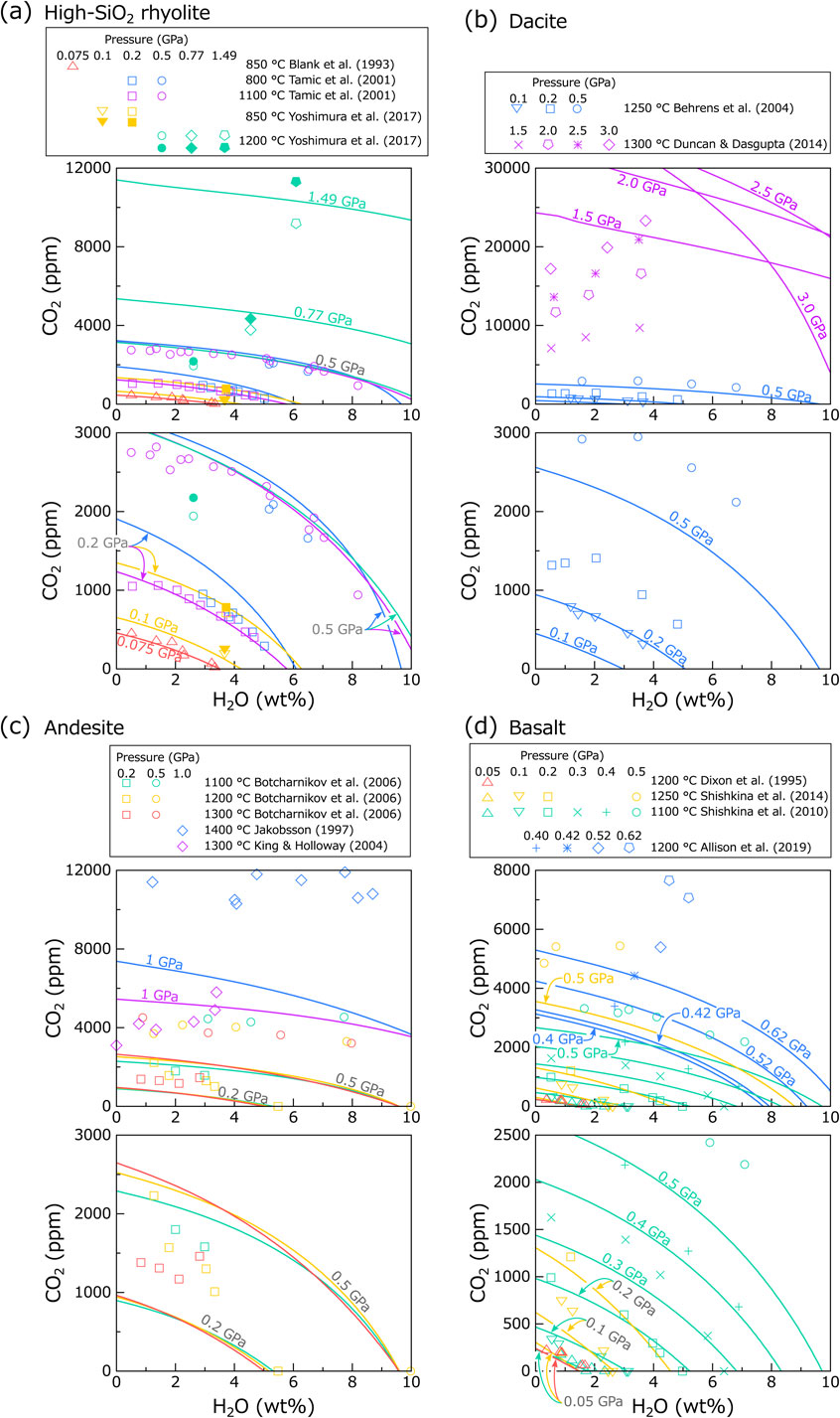
Figure 2a shows the experimental data and calculated isobars for high-SiO₂ rhyolitic melts. While Blank et al. (1993) and Tamic et al. (2001) reported that CO₂ dissolved solely as CO_2mol in their experimental samples, Yoshimura et al. (2017) observed presence of both CO_2mol and CO₃²⁻. Therefore, the data for CO_2mol + CO₃²⁻ are also shown for Yoshimura et al. (2017). The comparison shows that the data of Blank et al. (1993) and the 1100 °C data of Tamic et al. (2001) are reproduced well by the model with a deviation of ∼ 10%. The 800 °C data of Tamic et al. (2001), in particular those at 0.2 GPa, are less accurately reproduced (deviation is ∼ 25%), despite that all these data were used for calibrating the Duan (2014) model. The results of the 0.77 GPa experiment and 1.49 GPa experiment of Yoshimura et al. (2017), which were not used for the model calibration, are acceptably reproduced by the model with a deviation of ∼ 20%, whereas the 0.5 GPa experiment of Yoshimura et al. (2017) was less well reproduced by the model (with a deviation of ∼ 25%).

Figure 2b shows the comparison for dacitic melts (Behrens et al., 2004) and alkali-rich low-SiO₂ rhyolitic melts (Duncan and Dasgupta, 2014). In these melts, both CO_2mol and CO₃²⁻ exist as dissolved species. For dacitic melt (Behrens et al., 2004), the model significantly underestimates the CO₂ content (deviation is ∼ 40%), despite that these experimental data were used for the model calibration. For low-SiO₂ rhyolite (Duncan and Dasgupta, 2014), the model resulted in extremely high CO₂ content, which is clearly incompatible with the data. Moreover, the calculated isobars intersect each other despite the identical melt composition and temperature, which seems to be unrealistic for solubility behaviour.

Figure 2c shows the comparison for andesitic melts. These melts contain both CO_2mol and CO₃²⁻ as dissolved species. The CO₂ content of Botcharnikov et al. (2006) and Jakobsson (1997) is significantly higher than the calculated isobars, despite the data being used for the model calibration. The data of King and Holloway (2002) are to some extent consistent with the model.

Figure 2d shows the data for basaltic melts. All these melts contain solely CO₃²⁻ as dissolved species. It is known that CO₂ solubility in basaltic melt increases with increasing alkali and alkali earth content (e.g., Dixon, 1997; Moore, 2008), and the observation that the data of Shishkina et al. (2014) and Allison et al. (2019), both for alkali basalt, show much higher CO₂ content than the data of Shishkina et al. (2010), for tholeiitic basalt, is consistent with this relationship. The calculated isobars also show the same compositional dependency. However, the comparison shows that the model only reproduces well the experimental data for tholeiitic basalt (Shishkina et al., 2010) at <0.2 GPa with a deviation of ∼ 10%, and at higher pressures, the model failed to reproduce the data. For alkali basalt, the deviation is more severe at all pressure ranges.

In conclusion, the Duan (2014) model provides acceptable solubility prediction for rhyolitic melts (and tholeiitic melt at low pressures), whereas the model mostly underestimates the CO₂ content for other melts. Therefore, caution is required when applying the Duan (2014) model to dacite to alkali-rich basaltic melts. Nevertheless, the model can be used appropriately for natural andesitic to dacitic magmas because the interstitial melt of these magmas (or groundmass of the rocks) is typically high-SiO₂ rhyolitic in composition.

For reference, isobars calculated using Eq. (14) are compared with the experimental data (see Supplementary Document): it was found that the data fit did not improve significantly.

COMPARISON WITH THE SOLUBILITY MODEL MAGMASAT

Finally, the Duan (2014) model was compared with the MagmaSat model (Ghiorso and Gualda, 2015), which is similarly applicable to wide pressure and temperature conditions and various melt compositions (Fig. 3). The MagmaSat calculation was carried out using the VESIcal web application version 1.0.1 released by Iacovino et al. (2021).

Figure 3. Comparison between the Duan (2014) model and MagmaSat (Ghiorso and Gualda, 2015). (a) High-SiO₂ rhyolitic melts, (b) dacitic melts, (c) andesitic melts, and (d) basaltic melts. The solid line represents the isobars of Duan (2014), whereas the dashed lines represent the isobars of MagmaSat. Symbols are identical to those in Figure 2.

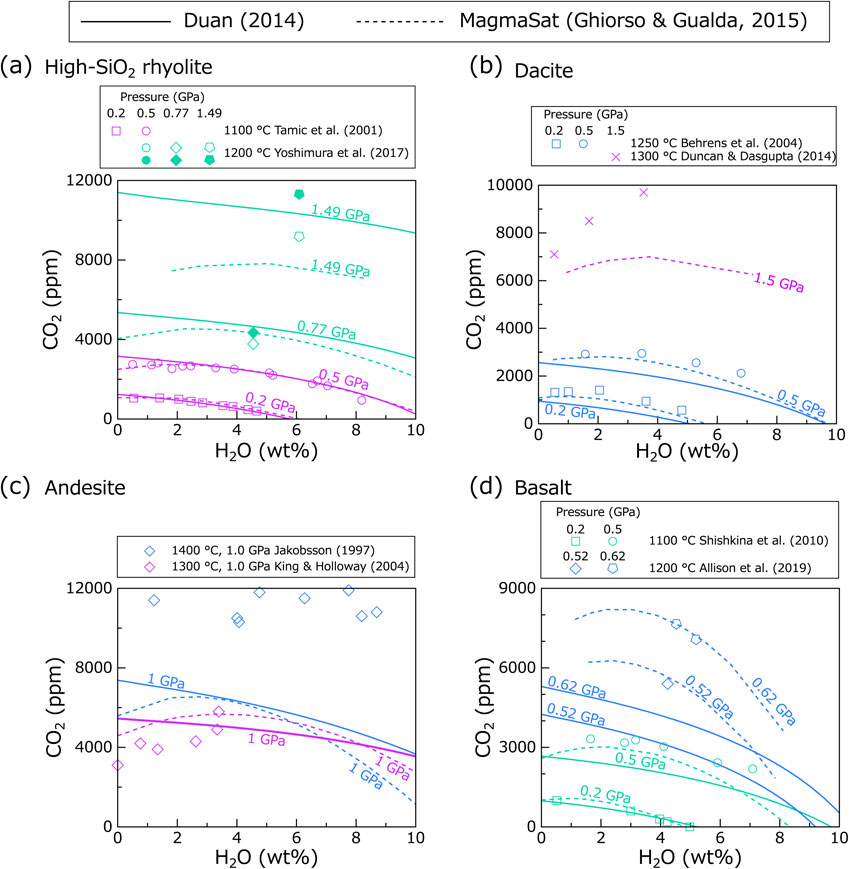
For rhyolite (Fig. 3a), both MagmaSat and Duan (2014) models generally accurately reproduce the experimental data. For the 1.49 GPa experiment (Yoshimura et al., 2017), MagmaSat underestimates the total CO₂ content (deviation is ∼ 25%), in contrast to the Duan (2014) model which acceptably reproduced the 1.49 GPa data (deviation is ∼ 10%).

For dacitic melt of Behrens et al. (2004) (Fig. 3b), MagmaSat results are more consistent with the data at 0.2 and 0.5 GPa than the Duan (2014) model. For low-SiO₂ rhyolitic melt of Duncan and Dasgupta (2014), MagmaSat well predicts the H₂O-poorest data (deviation is <10%). However, as the water content increases, the MagmaSat model significantly underestimates the CO₂ content.

For andesitic melts (Fig. 3c), data from King and Holloway (2002) are to some extent consistent with both models. Data from Jakobsson (1997) are reproduced by neither MagmaSat nor the Duan (2014) model.

For basaltic melts (Fig. 3d), data from the 0.2 GPa experiments are reproduced well by both models, whereas data from higher pressures (>0.5 GPa) are only reproduced well by MagmaSat. In particular, the data from Allison et al. (2019) for alkali basalt at high pressures (0.52 and 0.62 GPa) are excellently reproduced by MagmaSat, in contrast to the Duan (2014) model.

It can be concluded that MagmaSat appears to predict H₂O-CO₂ solubility better for most magmas. Therefore, MagmaSat can be seen as a safe choice to study, for example, pre-eruptive magmatic conditions based on melt inclusion data. Since the Duan (2014) model is simpler and provides reasonable solubility predictions at pressures of the shallow to middle crust for rhyolite and at pressures of the shallow crust for tholeiitic basalt, the model can be adequately used in simulation studies where the fundamental characteristics of degassing processes, rather than quantitative pressure estimation, are the main research target.

SUMMARY

This paper reviewed the solubility model developed by Duan (2014). The calculation procedure and some modifications of the calculation method for the partial fugacity coefficient at pressures >0.2 GPa were presented. The calculation results reproduced well those computed using the Windows executable file, which was previously provided on Duan’s website, within 2.5%. Comparing the model with experimental data showed that the Duan (2014) solubility model accurately predicted the solubility for high-SiO₂ rhyolitic melts, but it underestimated CO₂ content for other melts including dacitic, andesitic, and basaltic melts, especially when the pressure exceeded 0.5 GPa. Comparison with MagmaSat (Ghiorso and Gualda, 2015) revealed that MagmaSat provides values that are more consistent with experimental data than the Duan (2014) model. Therefore, MagmaSat may be preferred for quantitatively estimating magma chamber conditions based on melt inclusion data.

ACKNOWLEDGMENTS

I thank Junji Yamamoto and an anonymous reviewer for constructive comments. Editor Tetsu Kogiso carefully reviewed the manuscript and provided helpful suggestions. This study was supported by JSPS KAKENHI Grant Number JP20H01989.

SUPPLEMENTARY MATERIALS

Supplementary Document, code, and executable file are available online from https://doi.org/10.2465/jmps.221224b.

REFERENCES

• Albarède, F. (1995) Introduction to geochemical modeling. pp. 543, Cambridge University Press, Cambridge.
•  Allison,  C.M.,  Roggensack,  K. and  Clarke,  A.B. (2019) H₂O-CO₂ solubility in alkali-rich mafic magmas: new experiments at mid-crustal pressures. Contributions to Mineralogy and Petrology, 174, 58.
•  Baker,  D.R. and  Alletti,  M. (2012) Fluid saturation and volatile partitioning between melts and hydrous fluids in crustal magmatic systems: the contribution of experimental measurements and solubility models. Earth-Science Reviews, 114, 298-324.
•  Behrens,  H.,  Ohlhorst,  S.,  Holtz,  F. and  Champenois,  M. (2004) CO₂ solubility in dacitic melts equilibrated with H₂O-CO₂ fluids: Implications for modeling the solubility of CO₂ in silicic melts. Geochimica et Cosmochimica Acta, 68, 4687-4703.
•  Blank,  J.G.,  Stolper,  E.M. and  Carroll,  M.R. (1993) Solubilities of carbon dioxide and water in rhyolitic melt at 850°C and 750 bars. Earth and Planetary Science Letters, 119, 27-36.
•  Blank,  J.G. and  Brooker,  R.A. (1994) Experimental studies of carbon dioxide in silicate melts: Solubility, speciation, and stable carbon isotope behavior. Reviews in Mineralogy, 30, 158-186.
•  Botcharnikov,  R.E.,  Behrens,  H. and  Holtz,  F. (2006) Solubility and speciation of C-O-H fluids in andesitic melt at T=1100-1300 °C and P=200 and 500 MPa. Chemical Geology, 229, 125-143.
•  Dixon,  J.E. (1997) Degassing of alkalic basalts. American Mineralogy, 82, 368-378.
•  Dixon,  J.E.,  Stolper,  E.M. and  Holloway,  J.R. (1995) An experimental study of water and carbon dioxide solubilities in mid-ocean ridge basaltic liquids. Part I: calibration and solubility models. Journal of Petrology, 36, 1607-1631.
•  Duan,  X. (2014) A general model for predicting the solubility behavior of H₂O-CO₂ fluids in silicate melts over a wide range of pressure, temperature and compositions. Geochimica et Cosmochimica Acta, 125, 528-609.
•  Duan,  Z. and  Zhang,  Z. (2006) Equation of state of the H₂O, CO₂, and H₂O-CO₂ systems up to 10 GPa and 2573.15 K: Molecular dynamics simulations with ab initio potential surface. Geochimica et Cosmochimica Acta, 70, 2311-2324.
•  Duncan,  M.S. and  Dasgupta,  R. (2014) CO₂ solubility and speciation in rhyolitic sediment partial melts at 1.5-3.0 GPa - Implications for carbon flux in subduction zones. Geochimica et Cosmochimica Acta, 124, 328-347.
•  Ghiorso,  M.S.,  Carmichael,  I.S.E.,  Rivers,  M.L. and  Sack,  R.O. (1983) The Gibbs free energy of mixing of natural silicate liquids; and expanded regular solution approximation for the calculation of magmatic intensive variables. Contributions to Mineralogy and Petrology, 84, 107-145.
•  Ghiorso,  M.S. and  Gualda,  G.A.R. (2015) An H₂O-CO₂ mixed fluid saturation model compatible with rhyolite-MELTS. Contributions to Mineralogy and Petrology, 169, 53.
•  Gualda,  G.A.R.,  Ghiorso,  M.S.,  Lemons,  R.V. and  Carley,  T.L. (2012) Rhyolite-MELTS: a modified calibration of MELTS optimized for silica-rich fluid-bearing magmatic systems. Journal of Petrology, 53, 875-890.
•  Holloway,  J.R. and  Blank,  J.G. (1994) Application of experimental results to C-O-H species in natural melts. Review in Mineralogy, 30, 185-230.
•  Iacono-Marziano,  G.,  Morizet,  Y.,  Trong,  E. and  Gaillard,  F. (2012) New experimental data and semi-empirical parameterization of H₂O-CO₂ solubility in mafic melts. Geochimica et Cosmochimica Acta, 97, 1-23.
•  Iacovino,  K.,  Matthews,  S.,  Wieser,  P.E.,  Moore,  G.M. and  Bégué,  F. (2021) VESIcal Part I: An open-source thermodynamic model engine for mixed volatile (H₂O-CO₂) solubility in silicate melts. Earth and Space Science, 8, e2020EA001584.
•  Ihinger,  P.D.,  Zhang,  Y. and  Stolper,  E.M. (1999) The speciation of dissolved water in rhyolitic melt. Geochimica et Cosmochimica Acta, 63, 3567-3578.
•  Jakobsson,  S. (1997) Solubility of water and carbon dioxide in an icelandite at 1400 °C and 10 kilobars. Contributions to Mineralogy and Petrology, 142, 129-135.
•  King,  P.L. and  Holloway,  J.R. (2002) CO₂ solubility and speciation in intermediat (andesitic) melts: The role of H₂O and composition. Geochimica et Cosmochimica Acta, 66, 1627-1640.
•  Konschak,  A. and  Keppler,  H. (2014) The speciation of carbon dioxide in silicate melts. Contributions to Mineralogy and Petrology, 167, 998.
•  Liu,  Y.,  Zhang,  Y. and  Behrens,  H. (2005) Solubility of H₂O in rhyolitic melts at low pressures and a new emprical model for mixed H₂O-CO₂ solubility in rhyolitic melts. Journal of Volcanology and Geothermal Research, 143, 219-235.
•  McMillan,  P.F. (1994) Water solubility and speciation models. Reviews in Mineralogy, 30, 131-156.
•  Moore,  G. (2008) Interpreting H₂O and CO₂ contents in melt inclusions: constraints from solubility experiments and modeling. Reviews in Minralogy and Geochemistry, 69, 333-361.
•  Moore,  G.,  Vennemann,  T. and  Carmichael,  I. (1998) An empirical model for the solubility of H₂O in magmas to 3 kilobars. American Mineralogist, 83, 36-42.
•  Moore,  G.,  Roggensack,  K. and  Klonowski,  S. (2008) A low-pressure-high-temperature technique for the piston-cylinder. American Mineralogist, 93, 48-52.
•  Newman,  S. and  Lowenstern,  J.B. (2002) VolatileCalc: a silicate melt-H₂O-CO₂ solution model written in Visual Basic for excel. Computers & Geosciences, 28, 957-604.
•  Ni,  H. and  Keppler,  H. (2013) Carbon in silicate melts. Reviews in Mineralogy and Geochemistry, 75, 251-287.
•  Papale,  P. (1997) Modeling of the solubility of a one-component H₂O or CO₂ fluid in silicate liquids. Contributions to Mineralogy and Petrology, 162, 237-251.
•  Papale,  P. (1999) Modeling of the solubility of a two-component H₂O + CO₂ fluid in silicate liquids. American Mineralogist, 84, 477-492.
•  Papale,  P.,  Moretti,  R. and  Barbato,  D. (2006) The compositional dependence of the saturation surface of H₂O+CO₂ fluids in silicate melts. Chemical Geology, 229, 78-95.
•  Shishkina,  T.A.,  Botcharnikov,  R.E.,  Holtz,  F.,  Almeev,  R.R. and  Portnyagin,  M.V. (2010) Solubility of H₂O- and CO₂-bearing fluids in tholeiitic basalts at pressure up to 500 MPa. Chemical Geology, 277, 115-125.
•  Shishkina,  T.A.,  Botcharnikov,  R.E.,  Holtz,  F.,  Almeev,  R.R., et al (2014) Compositional and pressure effects on the solubility of H₂O and CO₂ in mafic melts. Chemical Geology, 388, 112-129.
•  Tamic,  N.,  Behrens,  H. and  Holtz,  F. (2001) The solubility of H₂O and CO₂ in rhyolitic melts in equilibrium with a mixed CO₂-H₂O fluid phase. Chemical Geology, 174, 333-347.
•  Wieser,  P.E.,  Iacovino,  K.,  Matthews,  S.,  Moore,  G. and  Allison,  C.M. (2022) VESIcal: 2. Acritical approach to volatile solubility modeling using an open-source python3 engine. Earth and Space Science, 9, e2021EA001932.
•  Yoshimura,  S. (2023) Carbon dioxide and water in the crust. Part 1: Equation of state for the fluid. Journal of Mineralogical and Petrological Sciences, 118, 022.
•  Yoshimura,  S.,  Nakamura,  M. and  Yurimoto,  H. (2017) Carbonate ions in high-SiO₂ rhyolite observed in fluid-melt equilibrium experiments. Geochemical Journal, 51, 251-262.
•  Zhang,  Y. (1999) H₂O in rhyolitic glass and melts: measurement, speciation, solubility, and diffusion. Reviews of Geophysics, 37, 493-516.
•  Zhang,  Y.,  Xu,  Z.,  Zhu,  M. and  Wang,  H. (2007) Silicate melt properties and volcanic eruptions. Reviews of Geophysics, 45, RG4004.