Journal of the Meteorological Society of Japan. Ser. II
Online ISSN : 2186-9057
Print ISSN : 0026-1165
ISSN-L : 0026-1165
Article: Special Edition on Typhoons in 2018-2019
Intensity and Structural Changes of Numerically Simulated Typhoon Faxai (1915) before Landfall
Yoshiaki MIYAMOTOHironori FUDEYASUAkiyoshi WADA
Author information
JOURNAL OPEN ACCESS FULL-TEXT HTML

2022 Volume 100 Issue 1 Pages 181-196

Details
Abstract

A numerical simulation of Typhoon Faxai (1915), which made landfall with a central pressure of 960 hPa in the Kanto region of Japan, was conducted using a nonhydrostatic numerical model with a 1-km grid spacing. Faxai sustained a symmetric structure until the landfall and caused severe damage due to strong winds. The simulation successfully simulated the realistic track and intensity of Faxai for 48 h around landfall. The simulated intensity was strong until the time of landfall, and the spatial size of the vortex was small. The structure of the simulated Faxai, identified as having an axisymmetric flow field and eyewall, was similar to that of a welldeveloped tropical cyclone (TC) in the tropics. Around the TC center, the surface latent heat flux was over 300 W m−2 until landfall, and the vertical wind shear was less than 9 m s−1 between the 1.5- and 12.0-km altitudes, which is relatively weak at midlatitudes. The maximum potential intensity (MPI) was calculated using environmental parameters around the simulated TC. The simulated and best track TC intensities exceeded the MPI for approximately 12 h before landfall, that is, the TC was in a superintense state. The superintensity was mainly caused by the presence of supergradient wind, which, in turn, resulted from the strong intensity and axisymmetric structure of the typhoon. The simulated TC satisfies the assumptions for the formulation of the MPI during the quasi-steady state, except for the gradient wind balance, implying that the structure of a TC is similar to that of a developed TC in the tropics. The present analyses suggest that the strong intensity of Faxai results from favorable environmental conditions and vortex structure.

1. Introduction

The energy source of tropical cyclones (TCs) is the underlying ocean, and thus TCs tend to intensify when they pass over regions with warm sea-surface temperature (SST). The latent energy provided by the ocean is converted into kinetic energy to drive the TC through condensation in the inner core. The spatial distribution of condensation heating and vortex structure are important to determine the rate of change in the TC intensity; diabatic heating located inside the radius of maximum wind (RMW), with more axisymmetric components and with a higher amplitude, favors TC intensification (Shapiro and Willoughby 1982; Schubert and Hack 1982; Nolan et al. 2007; Rogers et al. 2013; Shimada et al. 2017).

Emanuel (1986) and successive studies developed a theory for steady TCs by assuming an axisymmetric structure, thermal–wind balance, and neutrality for moist slantwise convection. The theory enables one to obtain an upper-bound intensity that a TC can potentially achieve in a given environment, which is referred to as the maximum potential intensity (MPI). It has been shown that the MPI can capture the upper-bound intensity of real TCs (DeMaria and Kaplan 1994; Emanuel 2000; Miyamoto et al. 2017). The theory has been further extended by Emanuel and Rotunno (2011) to represent the steady-state structure of TCs as well as the TC intensity by assuming an equilibrium of vertical mixing by Kelvin–Helmholtz (K–H) instability in the upper troposphere.

TCs seldom intensify or maintain their intensity when structural and environmental conditions are not favorable. The theories introduced above assume that the TC vortex has a vertically upright structure. Although the vertical wind shear of horizontal winds (VWS) is typically weak or moderate in the tropics1, most TCs are substantially influenced by strong VWS when they enter midlatitudes where the atmosphere is baroclinic because of the steep temperature gradient in the meridional direction. The VWS generally reduces TC intensity because it tilts the vortex structure and directly transports dry air into the TC core and boundary layer, which is the primary source of air for the eyewall (Jones 1995, 2000; DeMaria 1996; Frank and Ritchie 2001; Tang and Emanuel 2010; Riemer et al. 2010). Another major reason why TCs weaken at midlatitudes is the low SST. Because the amount of energy provided by the ocean decreases over the low SST region, TCs tend not to develop at midlatitudes compared with the tropics. Except for TCs that reintensify as an extratropical cyclone, most TCs weaken as they move to midlatitudes.

In 2019, Typhoon Faxai made landfall in the Kanto region, which includes Tokyo city, and caused severe damage to the Boso peninsula, located on the eastern side of central Tokyo. Faxai moved northward into Tokyo Bay and made landfall at Chiba Prefecture on September 9, 2019 (cf. Fig. 1), during which many buildings, including houses in the Boso peninsula, were damaged, resulting in a month-long shutdown of electricity in the peninsula. The intensity of Faxai at landfall, with a central pressure of 960 hPa, was the strongest out of the typhoons that have made landfall around the Kanto region since 1991. Furthermore, the structure of the clouds at the center of Faxai was relatively axisymmetric even when Faxai made landfall (cf. Fig. 1). It is scientifically crucial to explore the physical reason behind the sustenance of a strong intensity by the typhoon at midlatitudes.

This study aims to examine the crucial factors leading to Faxai maintaining its strong intensity up to landfall by focusing on the vortex structure. For this purpose, we conducted a numerical simulation of Faxai using a full-physics nonhydrostatic atmosphere model. The remainder of this paper is organized as follows. The experimental setting and methodology for the analyses are described in Section 2. The results of the simulation focusing on changes in intensity and structure before landfall are shown in Section 3 and discussed in Section 4. This study is summarized in Section 5.

2. Experimental settings and methodology of analysis

2.1 Experimental settings

We conducted a numerical simulation of Faxai using a nonhydrostatic model developed by the Japan Meteorological Agency (NHM, Saito et al. 2006). The simulation period was from 00 UTC, September 8 to 00 UTC, September 10, 2019, covering the period during which the typhoon approached the coast and made landfall. The computational domain covered 960 km × 1260 km, with a grid spacing of 1 km. The top of the numerical domain was at a height of approximately 27 km, and there were 55 vertical levels. The integration time was 48 h. The time step was 3 s for the NHM.

The Japan Meteorological Agency (JMA) mesoscale objective analysis with a horizontal resolution of 5 km was used for creating the atmospheric initial and lateral boundary conditions. We used the SST data from the Microwave Optimally Interpolated SST (OISST hereafter) daily product, obtained from the Remote Sensing Systems website (https://www.remss.com/). OISST is the daily merged satellite dataset that includes three satellite SST datasets measured by the WindSat, the Advanced Microwave Scanning Radiometers 2, and the Global Precipitation Measurement Microwave Imager. The nonhydrostatic atmosphere model includes microphysics expressed in an explicit three-ice bulk microphysics scheme (Ikawa and Saito 1991; Lin et al. 1983). Exchange coefficients for the air–sea momentum and enthalpy transfers over the sea were based on bulk formulas (Kondo 1975). The subgrid-scale turbulence and shortwave and longwave radiation were parameterized by a turbulent closure model (Klemp and Wilhelmson 1978; Deardorff 1980) and radiation scheme (Sugi et al. 1990), respectively. See Wada (2020) for details of the experimental setup.

2.2 Analysis

The track and intensity of the simulated TC were compared with the best track data to validate the simulation. The best track data for Faxai were obtained from the Regional Specialized Meteorological Center Tokyo. To compare the simulated TC structure, the observed data for radar reflectivity on 18 UTC, September 8 were used.

The center of the simulated TC was detected as a centroid using sea-level pressure (Braun 2002), which is a useful method to accurately detect the TC center, especially in datasets with high spatial resolution, by avoiding the detection of local pressure minima (caused by small-scale convection) instead of the vortex center (Nguyen et al. 2014). TC intensity was defined as the maximum tangential velocity averaged in the azimuthal direction at a 1.5-km altitude. Accordingly, the RMW was defined as the radius at which the maximum velocity was observed at a 1.5-km altitude. The VWS was calculated as follows:   

where Δv2,1 is the absolute value of the velocity difference at two levels, and u and v are the zonal and meridional velocities, respectively. Then, VWS was obtained by taking a spatial average between the 200-km and 500-km radius.

The structural change of the simulated TC was examined by introducing a parameter, axisymmetry, defined in Miyamoto and Takemi (2013),   

where r, λ, z, and t are the radius, azimuth, height, and time, respectively; φ is a quantity; the bar indicates the azimuthal average; and the prime indicates the deviation. As defined, γφ takes 0–1 values and γφ = 1 when φ is totally axisymmetric; φ′ = 0.

3. Results

3.1 Overview of the simulated TC

Figure 1 shows the best track of Faxai and that of the simulated TC. Faxai moved northwestward over the Kuroshio Current, approached the Kanto region, and made a landfall at Chiba Prefecture on September 9. Before the landfall, the track of the simulated TC was similar to the best track. The SST was higher than or equal to 301 K along the tracks of both best track and simulated TCs, except near the coast.

Fig. 1.

(Top) Best track of Faxai (gray line with circle), the track of the simulated TC (yellow line), and spatial distribution of SST (K), which was fixed during the simulation period (shaded). The numbers near the simulated track represent the time of simulation (day and hour) in UTC initiated from 00 UTC, September 8. The red circle indicates the time of landfall of the simulated TC. The panel covers most of the domain for the numerical simulation. (Bottom) Horizontal distribution of observed radar reflectivity (dBZ) for Faxai on 18 UTC, September 8.

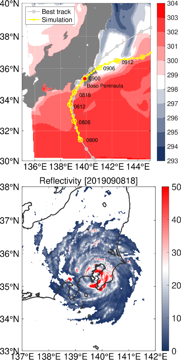
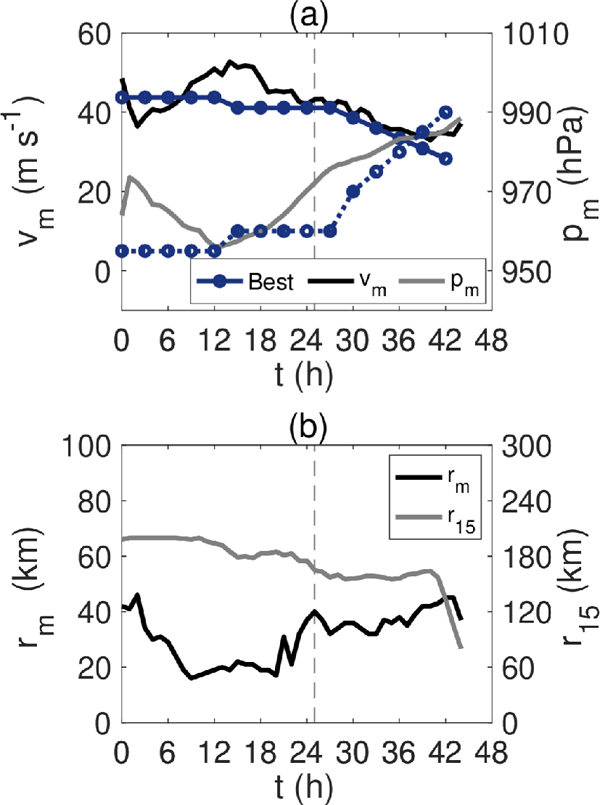
Figure 2a shows the time series of the TC intensity vm and sea-level pressure at the grid point of pressure centroid pm. The simulated TC intensified to t = 12 h and sustained a peak intensity of approximately 50 m s−1 for approximately 6 h before the intensity gradually decreased. The intensity of the simulated TC was weaker than the best track in the first several hours of simulation, which would be because the simulation was initiated from when the intensity of Faxai was strong and in the quasi-steady state, and the cloud structure was not represented at the initial time of simulation.

Fig. 2.

(a) Time series of best track intensity of Faxai (dark blue line with circle), maximum azimuthally averaged tangential velocity at z = 1.5 km vm of the simulated TC (black line), and minimum surface pressure (gray line). Note that the best track data are an estimate of the maximum surface wind speed. (b) Time series of the RMW (black line) and outer radius at which the azimuthally averaged tangential velocity is 15 m s−1, r15 (gray line) of the simulated TC. The radii were evaluated at the 1.5-km altitude. The vertical thin dashed lines in both panels indicate the time of landfall of the simulated TC.

Figure 2b shows the time series of the RMW and the radius at which the azimuthally averaged tangential velocity was 15 m s−1 outside the RMW, r15. The RMW decreased from 40 km to 20 km in the first 10 h of simulation and was approximately constant for 10 h, before increasing to 40 km after t = 20 h. r15 was approximately 200 km at the start and then gradually decreased with time.

Figure 3 depicts the horizontal cross section of total hydrometeor qt, vertically averaged between z = 1.5 km and 12 km and horizontal wind at z = 1.5 km, at six selected times (t = 6, 12, 18, 24, 30, and 36 h). At t = 6 h, there was a ring-shaped cloud surrounding the eye around a radius of 20 km. We can regard the ringshaped cloud as an eyewall. The eyewall was particularly prominent from t = 12 h to 30 h before becoming unclear, which is consistent with the radar image as shown in Fig. 1. Another notable feature was the spiral rainband extending from r ≈ 70 km from the north of the center to r ≈ 180 km southwest of the center at t = 6 h, which propagated cyclonically thereafter. There were a number of convective cells associated with the rainband from t = 12 h to 24 h. Because the time of landfall of the simulated TC was t = 25 h, the convection outside the core, especially in the northern side, appeared to be largely affected by orography during this period. The shape of the rainband seemed to be a ring rather than a spiral which had a peak of qt around = 60 km at t = 18 h. The eyewall appeared to be expanded to a large radius from t = 24 h to 30 h.

Fig. 3.

Horizontal cross section of the vertically averaged mixing ratio of total hydrometeor qt (g kg−1, shaded) and the horizontal wind at z = 1.5 km (vectors) at six selected times (t = 6, 12, 18, 24, 30, and 36 h). qt is averaged from z = 1.5 km to 12 km.

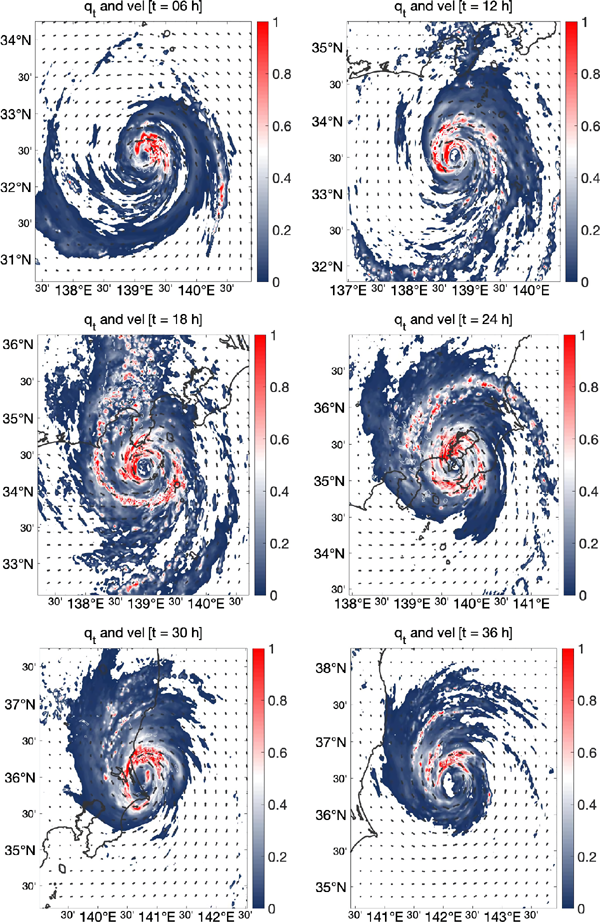
Figure 4 depicts the radius–height cross section of azimuthally averaged qt, tangential velocity v, and radial velocity u at the six selected times. A strong peak of qt was present around the RMW at all times, and the magnitude was large, especially at t = 12, 18, and 30 h. At t = 12 h and 18 h, there was another peak of qt outside the RMW; the peak was located around r = 40 km at t = 12 h and r = 60 km at t = 18 h, which was consistent with the ring-shaped cloud outside the RMW, as shown in Fig. 3. The secondary peak of qt appeared to merge with the eyewall located around the RMW at t = 24 h. The peak of qt decayed at t = 36 h when the simulated TC weakened (cf. Fig. 2b).

Fig. 4.

Radius–height cross section of qt (g kg−1, shaded), v (black contour), and u (gray contour) at six selected times (t = 6, 12, 18, 24, 30, and 36 h). The quantities were azimuthally averaged. The contour interval for v is 10 m s−1, whereas that for u is 5 m s−1. Negative values for velocities are indicated by dashed lines.

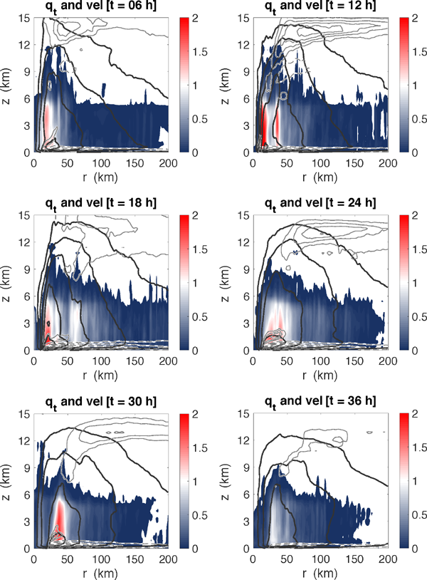
The peak of v was located around the 1-km altitude and decayed in the vertical and radial directions at all times shown in the figure. After the merging of the inner and outer peaks of qt at t = 24 h, the RMW increased. The inflow and outflow were strong immediately above the ocean surface and in the layer between z = 12 km and 14 km, respectively. The spatial distribution of tangential and radial velocity was consistent with that in previous studies focusing on TCs in the tropics (e.g., Chavas et al. 2015).

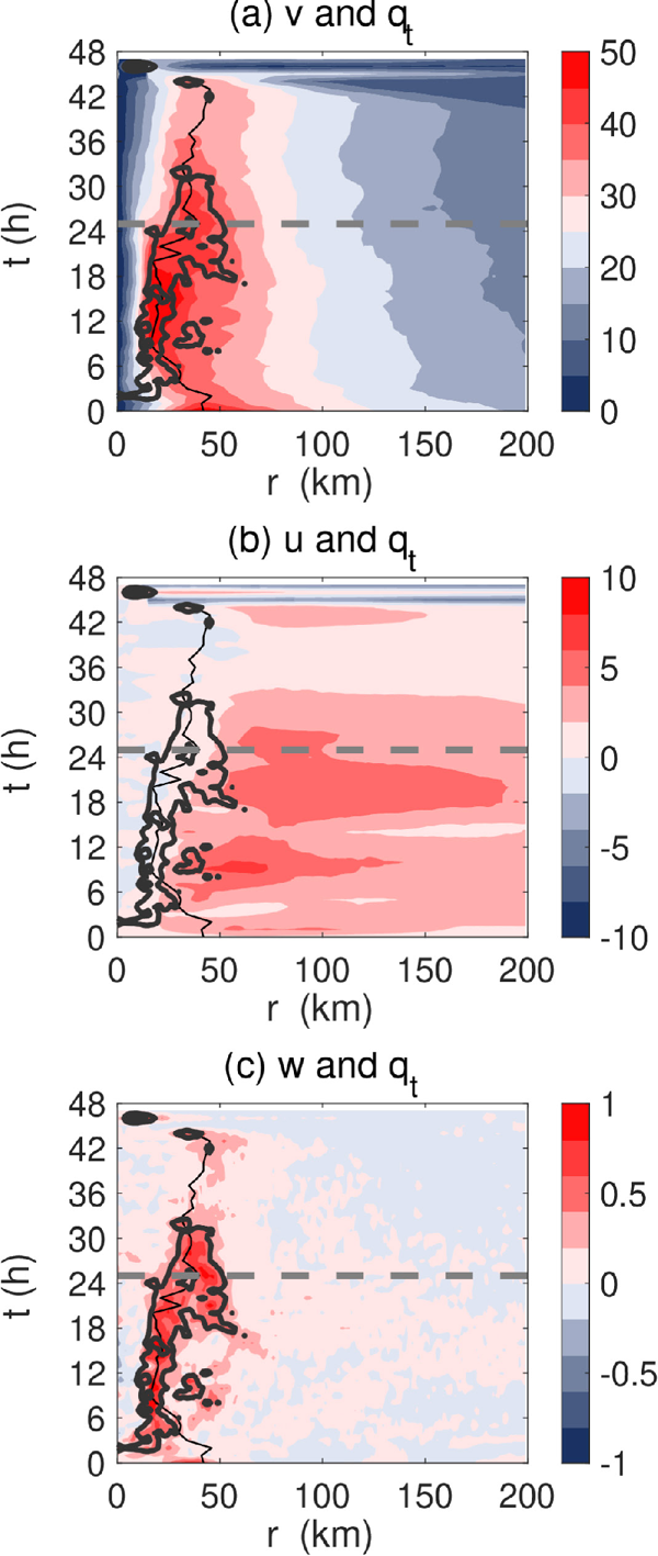
Figure 5a displays the radius–time cross section of v at z = 1.5 km and vertically averaged w and qt from z = 1.0 km to 10.0 km, all of which were averaged azimuthally. v at the outer radii did not significantly change in time before t = 24 h, whereas v decayed at all radii afterward. It should be noted that because the simulated TC moved out of the numerical domain at t = 45 h, the data for the last several hours are not meaningful.

Fig. 5.

Radius–time cross section of qt (g kg−1, contour) and velocity (shaded): (a) tangential velocity v (m s−1), (b) radial velocity u (m s−1), and (c) vertical velocity w (m s−1). The contour interval for qt is 0.5 g kg−1. The quantities were azimuthally averaged. v was evaluated at 1.5 km. w and qt were vertically averaged from z = 1.0 km to 10.0 km, and u was averaged from z = 10.0 km to 13.0 km. The thick black line indicates the RMW at z = 1.5 km.

Figure 5b displays the radius–time cross section of u averaged from z = 10.0 km to 13.0 km and qt averaged from 1.0 km to 10.0 km, both of which were averaged azimuthally. u in the upper layer was mostly positive and large until t = 30 h. Specifically, there were a few events in which u was large, with the peak of u located outside the large qt region. A large u region radially covered hundreds of kilometers.

w was large around the RMW (Fig. 5c). The radius of the maximum w was initially small but gradually increased. qt was large where w was large. Both w and qt decreased after t = 24 h, which was consistent with the TC intensity (cf. Fig. 2b). The temporal variation of u appeared to be associated with those of w and qt.

Figure 6a shows the time series of the VWS calculated by (1) using levels of 1.5 km and 12 km as typically done by previous studies (Chen and Zhang 2013; Miyamoto and Nolan 2018). The VWS was initially 9.0 m s−1, after which it reduced to 7.3 m s−1 at t = 4 h, increased to 10 m s−1 at t = 20 h, which is 5 h before the landfall, and then sustained this value afterward. Compared with the time series of the TC intensity (cf. Fig. 2a), the period in which the simulated TC obtained the strong intensity corresponds to that for VWS less than 9 m s−1. The VWS was less than 10 m s−1 until the landfall, which is not large when compared with the typical values at midlatitudes. We conducted an analysis to calculate the VWS between 200 hPa and 850 hPa around TCs approaching the midlatitudes in the north-western Pacific using the best track data and reanalysis data (JRA-55, Kobayashi et al. 2015; Harada et al. 2016). The mean VWS around the TCs in the north-western Pacific when they are located at latitudes higher than 30 deg was 16.6 m s−1.

Fig. 6.

(a) Time series of VWS defined as (1) and calculated between z = 1.5 km and 12 km. (b) Time series of fluxes for latent heat (black line) and sensible heat (gray line) averaged inside the 100-km radius from the TC center. (c) Time series of symmetry defined as (2) for the vertical vorticity ζ (black line) and qt (gray line) that were averaged from the center to the RMW and from z = 1.5 km to 10 km.

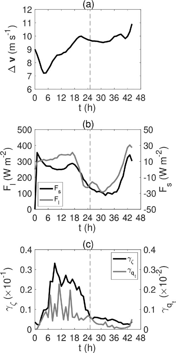
The time series of surface heat fluxes averaged around the TC center are shown in Fig. 6b. Because the TC intensity was sensitive to the energy flux at the ocean surface within a few to several times the RMW (Xu and Wang 2010; Miyamoto and Takemi 2010), the sensible and latent heat fluxes were averaged inside the 100-km radius. Both the latent heat and sensible heat fluxes were large until t = 18 h and then rapidly decreased, whereas they increased after t = 38 h. From t = 21 h to 39 h, when the simulated TC was close to or passed over the land, the sensible heat flux was negative, which indicates that the surface temperature was lower than the temperature at the level of the lowest atmosphere. The rapid decrease in the heat fluxes at t = 21 h appears to be because the simulated TC approached the land and partially because the SST decreased near the coast (cf. Fig. 1). Despite the decrease in the heat fluxes, the TC maintained its intensity for several hours, with the maximum wind speed only gradually decreasing (cf. Fig. 2a). Because the momentum flux is expected to increase due to the landfall, the enthalpy flux needs to be even larger than that over the ocean in order to sustain strong winds, from an energy–balance perspective (Emanuel 1986). The maintenance of the TC intensity after the landfall would result from physical processes that accelerate the tangential velocity in the TC core (Kitabatake and Tanaka 2009; Tsujino and Tsuboki 2020). On the other hand, the minimum sea-level pressure rapidly increased after t = 20 h, which appears to be due to the rapid decrease in the surface heat fluxes. The increase in the heat fluxes after t = 38 h was because the simulated TC moved back over the warm ocean.

Figure 6c shows the time series of the symmetry defined in (2) for the vertical component of relative vorticity ζ and qt, averaged radially from r = 0 to rm and vertically from z = 1.5 km to 10 km. The symmetry for ζ increased until t = 9 h and decreased from t = 18 h to 25 h. The decrease in the symmetry for ζ appears to be due to the effects of land. The symmetry for qt increased until t = 6 h, exhibited large fluctuations until t = 16 h, and decreased after the landfall. This indicates that the TC structure was relatively axisymmetric from t = 7 h to 20 h, as implied by the horizontal sections. The decrease in symmetry after t = 20 h might be due to the landfall, which changes the TC structure.

3.2 Maximum potential intensity

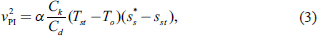
It is shown in the present analysis that the environmental conditions for the simulated TC are favorable. Hence, it is suggested that the MPI is large in the environment of Faxai, which would also be a reason for the strong intensity of Faxai. The formula for the MPI developed by Emanuel is given below (Bryan and Rotunno 2009; Miyamoto et al. 2017):   

where α = Ts/To, Ck, and Cd are the exchange coefficients for enthalpy and momentum at the ocean surface, T is the temperature, s is the moist entropy, and the asterisk represents the saturated value. The subscripts s, o, and st represent the ocean surface, outflow region, and surface layer, respectively. We calculated the MPI using environmental parameters at the initial state, i.e., before the environment was altered by the TC. Strictly speaking, the environment was affected by the TC at the initial time of simulation. However, if the time at which the MPI is evaluated is further before the initial time, the environment would be different from that when the TC approached the land. Hence, the MPI was calculated at the initial time of simulation based on the methodology by Bister and Emanuel (2002), whose the code is available online (http://texmex.mit.edu/pub/emanuel/TCMAX/). The ratio of surface exchange coefficients, Ck/Cd, which is one of the most important but unknown parameters, was fixed at 0.9 as that is the default value in the code and in the range of laboratory and field observations (Donelan et al. 2004; Bell et al. 2012; Takagaki et al. 2012). It should be noted that the values of the ratio are still under discussion, especially under high-wind conditions.

Figure 7 depicts the horizontal distribution of the MPI at the initial time of simulation (t = t0) at 00 UTC, September 8. Overall, the MPI correlated with the SST (cf. Fig. 1); the MPI was large in low latitudes and decreased with increasing latitude. The observed and simulated TCs passed over areas with high MPI (> 40 m s−1) and moved into low-MPI regions. After the landfall, the MPI was generally weak along the tracks.

Fig. 7.

Horizontal distribution of the MPI calculated by (3) at 00 UTC, September 8, when the simulation was initialized. The unit is m s−1. The yellow and gray lines represent the track of the simulated TC and best track.

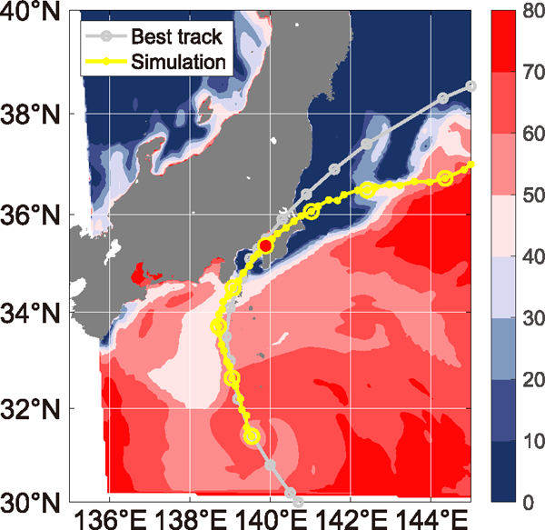
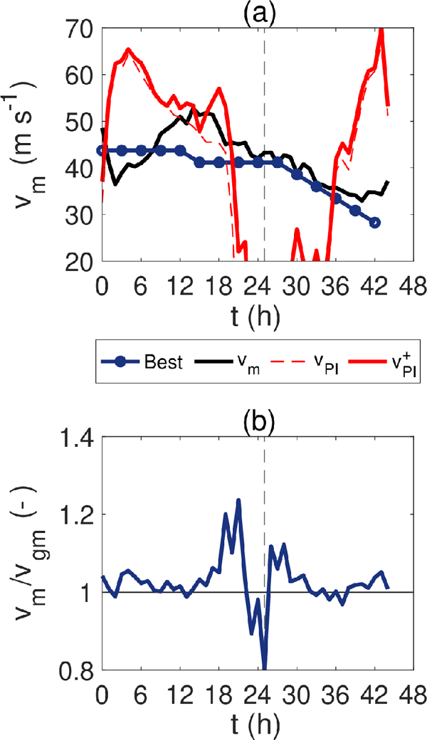
Figure 8 shows the MPI around the TC center at each time, as well as the time series of intensities of the simulated TC the best track. The MPI was evaluated at the initial time of simulation (t = t0) when the environment was not strongly affected by the TC, and the values of MPI at the grid point of the TC center every 1 h, which are denoted in Fig. 7, were plotted. When t = 4 h, the MPI was approximately 64.3 m s−1, which was approximately 25 m s−1 greater than the intensity of the simulated TC at this time. However, the MPI decreased with time afterward and after t = 10 h, the intensity of the simulated TC exceeded the MPI. This state lasted for more than 12 h until the simulated TC made landfall. The MPI was smaller than the simulated intensity until the simulated TC moved back over the warm ocean after t = 40 h. Thus, it is indicated that the simulated TC was in a superintense state, in which the TC intensity was greater than the MPI (Persing and Montgomery 2003) before landfall. Meanwhile, it should be noted that the MPI steadily decreased with time before the landfall, indicating that the environment changed along the track. Also note that the MPI was calculated from the quantities at the initial time of simulation, i.e., t = 0 h and interpolated spatially to get the value at the TC center. Because the initial field would possibly be affected by the presence of Faxai in the global analysis with typhoon bogusing, the MPI values for the first few hours would not represent the environmental potential. TCs respond to the changing environment on a certain time scale (not instantaneously), which might play a role in causing the difference between the simulated TC intensity and MPI.

Fig. 8.

(a) Time series of intensity of the simulated TC (black line) and best track (dark blue line). MPI vPI (3) is shown by the red dashed line. The modified MPI v+PI (4) is denoted by the solid red line. The MPIs were evaluated at the center of the simulated TC. (b) Time series of the ratio of vm to maximum velocity satisfying the gradient wind balance, vgm.

It has been reported that the MPI calculated by (3) may underestimate TC intensity under some circumstances (Persing and Montgomery 2003). Bryan and Rotunno (2009) analytically showed that the underestimation is mainly due to the assumption of gradient wind balance. By removing this assumption, they successfully derived the following formula for the maximum TC intensity, which captures the upperbound intensity of TC, whose intensity exceeds the MPI (3).   

where   
where η = ∂zu − ∂rw is the azimuthal vorticity, and the subscript m represents the value at the RMW and the height of the maximum tangential wind that is azimuthally averaged (HMW). Thus, by allowing agradient winds, the MPI equation (3) is modified. The modified equation includes the term β, which was determined by the TC internal structure. Particularly, when the tangential velocity was higher than the gradient wind speed (supergradient wind), β tended to be large and v+PI > vPI.

Figure 8a shows that v+PI was greater than vPI and close to the maximum intensity of estimated and simulated TCs. Thus, the upper-bound intensity was well captured by v+PI by considering supergradient winds in the core region. This indicates that the tangential velocity around the RMW and HMW of the simulated TC was faster than that satisfying the gradient wind balance, which enabled the TC to achieve an intensity greater than the MPI.

Figure 8b shows the times series of the ratio of vm to the maximum velocity satisfying the gradient wind balance vgm. The ratio exceeded 1.0 from t = 15 h to 20 h, indicating that the tangential velocity is greater than that satisfying the gradient wind balance, i.e., supergradient, in this period. It also implies that vm and v+PI exceeding vPI would be due to the presence of supergradient winds in the core region.

The MPIs calculated from the initial fields of the numerical simulation seem to be weaker than those obtained by previous studies. By comparing with the MPI calculated from Jordan (1958)'s tropical mean sounding, at the same SST, the MPIs calculated from the initial field are, in general, weaker than those from Jordan's sounding (figure not shown). Thus, the sounding at the initial time is not favorable for TCs to obtain a strong intensity compared with that in the tropics. The relatively weak MPI at a given SST would be because the quantities in the initial data are affected by the presence of the TC itself.

3.3 Structure during the quasi-steady period

The simulated TC had a strong intensity and an axisymmetric structure with a warm core, even though it was located at midlatitudes. Additionally, the TC intensity exceeded the MPI, the theory of which was developed for idealized atmospheric conditions in the tropics and did not include the effects of VWS or baroclinicity, which tend to weaken the TC intensity and are often strong at midlatitudes. As a result, it is expected that, in general, TCs may not reach the MPI at midlatitudes. Hence, we examined the reason why the simulated TC was strong, with an intensity greater than the MPI.

TCs appear to reach the MPI when the factors that play a negative role in determining the TC intensity are small and when assumptions to derive the MPI formula are satisfied. Hence, the result implies that the structure of the simulated TC when the intensity was comparable with or greater than the MPI (cf. Fig. 8) satisfied the assumptions. The basic assumptions of the theory are an axisymmetric structure, thermal wind balance in the free atmosphere, and neutrality of moist slantwise convection. Figure 9a displays the radius–height cross sections of azimuthally averaged u, v, and qt during the quasi-steady state, which was defined from t = 8 h to 18 h. As seen in the snapshots (Fig. 4), the maximum v was located around r = 20 km and z = 1 km. Strong inflow and outflow were present near the surface and tropopause, respectively. qt was large along the RMW, especially below z = 6 km. Furthermore, the RMW line was approximately collocated with the M surface that passed the RMW at z = 1.5 km, which is denoted as Mm.

Fig. 9.

Radius–height cross section of (a) v (black contour), u (gray contour), and qt (g kg−1, shaded), (b) M (gray contour) and s* (J K−1 kg−1, shaded) during the quasi-steady state. The thick gray line shows the RMW at each altitude, and the thick blue line represents a constant M line passing through the RMW at z = 1.5 km. The contour intervals for v, u, and M are 10 m s−1, 5 m s−1, and 1 × 10⁶ m2 s−1. Negative values for u are indicated by dashed lines.

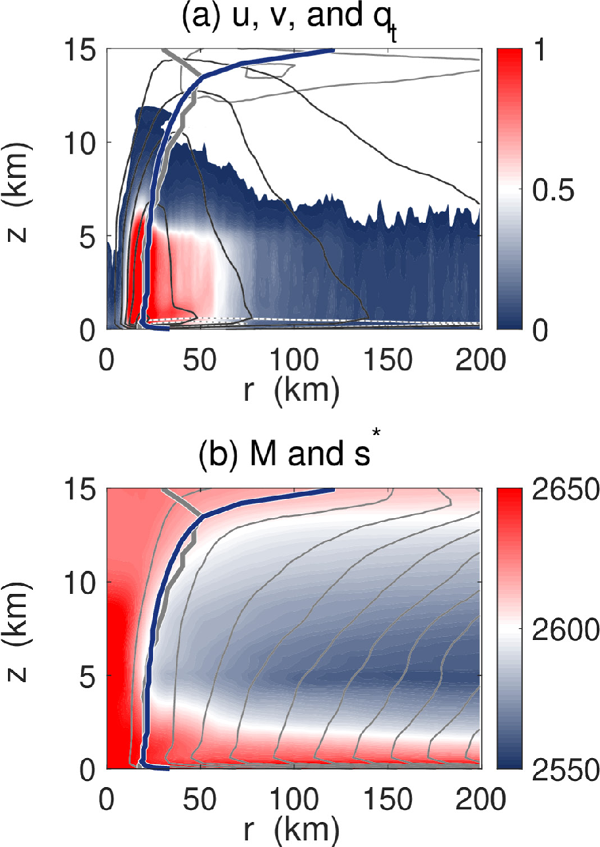
Figure 9b displays the radius–height cross sections of azimuthally averaged M and s* during the quasisteady state. s* was large near the surface, inside the RMW, and in the upper troposphere. M increased with the radius at all altitudes. The radii of the M surfaces did not vertically change greatly in the lower to middle free atmosphere, whereas the surfaces became horizontal in the upper layer. The M surfaces were almost congruent with the s* surfaces around the RMW.

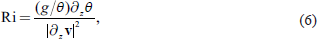
Emanuel and Rotunno (2011, hereafter ER11) developed a theory for the radial structure of angular momentum (tangential wind) by adding a closure for the vertical gradient of saturated moist entropy s* in the outflow to the original theory. They assumed that K–H instability always occurs along M surfaces in the outflow layer in the upper troposphere, which results in the vertical gradients of quantities keeping constant values through mixing. K–H instability occurs when the Richardson number, Ri, is less than the critical value. ER11 set the critical value to 1.0 in the outflow layer. Here, Ri is defined as the ratio of the squared Brunt–Väiälä frequency N2 = (g/θ) zθ to the squared VWS:   

where θ is the potential temperature and v is the vector of horizontal velocity. This results in a relationship between the vertical gradients of M and s* and radial distribution of 
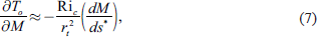
M, which is Eq. (31) of ER11.   
where rt is a radius at which the tangential velocity is 0 along an M surface. The assumption of self-stratification yields the approximate form of the radial distribution of 
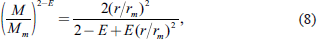
M at the top of the boundary layer as (Eq. 36 of ER11) follows:   
where Mm is the absolute angular momentum at the RMW and E = Ck/Cd. Because M ≡ rv + fr/2, the radial distribution of v is determined by Eq. (8).

Tao et al. (2019) verified the assumptions for the theory based on numerical simulations with different settings. Although it was shown that the assumptions work well in the simulated TCs, more verifications, especially based on real TCs, are desired. To examine the assumption for moist slantwise neutrality in the simulated TC, Fig. 10a depicts azimuthally averaged s*, T, and Ri on the Mm surface at each time. Before t = 21 h, s* was large, especially in the lower and upper layers, whereas it was small after t = 21 h. Nevertheless, the variation of s* was small along the Mm surface during the quasi-steady state from t = 8 h to 18 h. Figure 10b shows the relationship between M and s* at z = 1.5 km and from 30 km to 50 km, corresponding approximately to the range from 2 × RMW to 3 × RMW and to the lowest level of the free atmosphere. s* decreased with M, which is consistent with Tao et al. (2019).

Fig. 10.

(Top) Azimuthally averaged saturation entropy s* (J K−1 kg−1, shaded), T (black contour), and Ri = 1.0 (thick blue contour) on the surface of Mm. The contour intervals for T are 10 K. The horizontal axis represents the vertical grid number above z = 1.5 km. (Bottom) Scatter plot of M and s* in the region from 30 km to 50 km at z = 1.5 km, which are temporally averaged during the quasi-steady period.

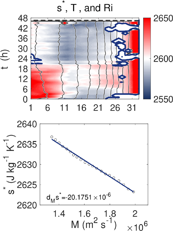
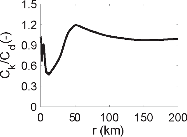
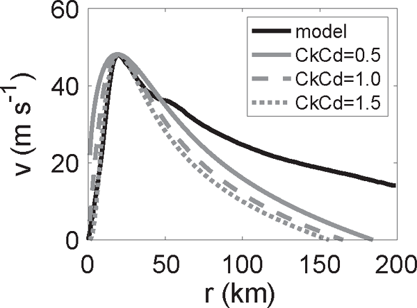
Figure 11 shows the radial profile of v at z = 1.5 km in the numerical simulation and analytical solutions (8) with three different parameters Ck/Cd, 0.5, 1.0, and 1.5. Overall, the analytical solution captured the spatial distribution of tangential velocity simulated in a numerical model inside the 50-km radius; the velocity increased with the radius inside the RMW and then gradually decreased with the radius outside. The maximum v did not depend on Ck/Cd as indicated by (8). However, the analytically obtained solutions for v by ER11 were significantly less than the velocity of the simulated TC, particularly outside the 50-km radius.

Fig. 11.

Radial profiles of tangential velocity at z = 1.5 km averaged azimuthally and temporally during the quasi-steady period (black line) and analytical solutions of ER11 theory (8) with three different values of Ck/Cd (gray lines). The gray solid, dashed, and dotted lines represent the solutions with Ck/Cd = 0.5, 1.0, and 1.5, respectively.

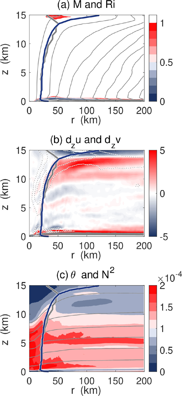
To explore the reason for the large deviation of the analytically obtained profile of tangential velocity from the simulated one, radius–height cross sections for Ri and M are depicted in Fig. 12a. Ri is smaller than 1.0 above z = 14 km inside the Mm surface. Along the Mm surface, Ri was less than 1.0 in the outflow region around the radius of 150 km for a few hours (cf. Fig. 10a), whereas the area was small. Ri along the Mm surface in the temporally averaged radius–height cross section is greater than 1.0. Figure 12b depicts the radius–height cross sections for vertical shear of radial wind dzu and vertical shear of tangential wind dzv. dzu was positive and large above the inflow layer (z > 1.0 km) and below the strong outflow region (z < 13.0 km). On the other hand, dzu was negative near the surface and in the upper layer (z > 13.0 km). dzv was negative except near the surface and was large, especially along and inside the RMW. Figure 12c displays the radius–height cross sections for N2 and θ. θ was large in the upper layer, and the vertical gradient of θ was large, especially inside the RMW. N2 was small in the upper layer. This indicates that the small Ri in Fig. 12a results from both the small N2 and large vertical shear of radial and tangential velocities. Nevertheless, the area where Ri is less than the critical value was small (Fig. 12a), implying that the parameterized turbulent mixing is small. Note that the parameterization for turbulence mixing does not utilize a critical Richardson number. Hence, the self-stratification assumption in the upper layer appears to be one of the causes of the large deviation of the simulated radial profile of tangential velocity from the theoretical profile of ER11.

Fig. 12.

(a) Radius–height cross section of Ri as defined by (6) (shaded) and M (contour), (b) vertical shear of radial velocity (× 10−3 s−1, shaded) and tangential velocity (contour), and (c) θ (K, contour) and N2 (s−2, shaded). The contour intervals for M, dzv, and θ are 1 × 10⁶ m2 s−1, 1 × 10⁻³ s−1, and 10 K. They are calculated by the quantities averaged azimuthally and temporally during the quasi-steady period.

4. Discussion

The analyses for the simulated Faxai indicate that the TC sustained a relatively strong intensity just before landfall. The strong intensity appears to be most likely due to the following favorable environmental conditions: relatively low VWS for midlatitudes and large surface flux for latent heat. Because the intensity of the simulated TC weakens immediately after the surface heat flux decreases around the TC center and the VWS increases, it is suggested that the simulated TC is intensified mainly by the large heat flux under an environment with low VWS. The reduction in surface heat flux is associated with the landfall of the simulated TC and also with the low SST near the coast (cf. Fig. 1). Hence, the favorable conditions for TC development appear to last until the TC center reaches the coastal region.

The favorable environmental conditions would result in the simulated TC having a structure of typical developed TCs in the tropics: well-defined eye and eyewall; axisymmetric vortex structure; strong secondary circulation, including strong surface inflow, vertical motion around the RMW, and outflow in the upper layer; and rainbands. The present analyses suggest that the strong intensity was due to favorable environmental conditions and a well-developed TC structure.

The maximum intensity of the simulated TC is greater than that determined by the environment for about 12 h before landfall. The modified MPI, which considers supergradient winds, better captures the maximum intensity. This implies that the strong intensity of the simulated TC is due to its inner core structure as well as the environmental conditions. By analyzing TCs simulated in a global nonhydrostatic model, Miyamoto et al. (2014) showed that tangential velocity tended to be supergradient when the TC intensity was strong, the RMW was large, and the flow structure was axisymmetric. Hence, the supergradient winds of the simulated TC would result from the strong TC intensity and axisymmetric structure.

It should be noted that, although Miyamoto et al. (2014) showed that TCs with large RMW tended to result in supergradient winds, the RMW of the simulated TC was relatively small2. In contrast, a small RMW is favorable for producing an intense TC for the following reasons: TCs with small RMW likely cause weak ocean mixing and less SST cooling (Lin et al. 2009; Price 2009; Miyamoto et al. 2017; Wada and Chan 2021), tend to be axisymmetric, have large inertial stability that results in high efficiency of kinetic energy production from condensation, and require less water vapor to produce condensation for all azimuths at a given radius. In fact, the simulated TC had a strong intensity and axisymmetric diabatic heating around the RMW, whereas the ocean cooling processes were not considered in the simulation. Thus, a small RMW would help produce a strong intensity in this case.

The simulated TC during the quasi-steady state satisfies key assumptions for Emanuel's MPI theory, which has been developed for tropical conditions, whereas the TC is located at midlatitudes. The analyses of the simulated TC suggest that the structure of Faxai was favorable for the development of TC until just before landfall. It should be noted that the analytically derived radial distribution of tangential velocity does not capture the simulated distribution. A possible cause of the difference is that Ri is less than 1.0 only in a small area (cf. Fig. 12a). According to ER11, the condition, Ri < 1.0, is satisfied along many M surfaces in the outflow layer. However, the region in which Ri < 1.0 in the simulated TC is small. The large Ri in the upper troposphere has also been observed in the simulated Hurricane Patricia (2015) as shown by Tao et al. (2019). They pointed out possible reasons for the cause of the difference from the analytical solution, which are associated with (1) radially constant Ck/Cd, (2) simplified boundary–layer processes, (3) threedimensional processes that are neglected by the theory, and (4) the neglected radial component of the vertical wind shear. In fact, Ck/Cd in the simulated TC varies in the radial direction during the quasi-steady state (Fig. 13), which has been assumed to be constant in the theoretical calculation. On the other hand, Tao et al. (2019) also showed in their idealized simulations that the Ri is small in the upper layer in accordance with the theory, whereas the deviation of the radial profile of tangential velocity in their idealized simulation from the theoretically obtained one is not negligible especially in the outer region. Further investigations are required to determine the cause of difference and to obtain analytical solutions that provide radial profiles of tangential velocity close to the observed or modeled TCs.

Fig. 13.

Radial profile of Ck/Cd for the simulated TC, which is averaged in the azimuthal direction and in time from t = 8 h to 18 h. Only values over the ocean were used to take an average.

5. Conclusions

We conducted a numerical simulation of Faxai using a nonhydrostatic model with a grid spacing of 1 km. The simulated TC intensified to a maximum intensity of ∼ 50 m s−1 over several hours, which is approximately the same as the observed maximum intensity of Faxai, although the level at which the intensity was evaluated was 1.5 km, which is different from that for the best track intensity. The maximum intensity was sustained until the simulated TC approached the coastal region and decreased thereafter. The reason that the TC developed a strong intensity was examined by analyzing both environmental factors and the internal vortex structure. The environmental conditions were favorable for TC development; the VWS was small compared with typical values at midlatitudes, and the area-averaged surface heat flux around the TC center was large. Furthermore, the simulated TC had a well-developed structure typical of that observed in the tropics, especially during the quasi-steady state.

Both the simulated and observed TC intensities exceeded the MPI calculated by the initial field of simulation, implying that Faxai was in a superintense state for several hours before landfall. The intensity was better captured by the analytically obtained intensity considering the supergradient wind. This indicates that the superintensity was attained by the strong intensity and axisymmetric structure.

By examining the assumptions for the MPI theory, it was revealed that the assumptions were valid during the quasi-steady state of the simulated TC. Hence, the intensity of the simulated TC would be close to or even stronger than that of the MPI. This suggests that the strong intensity of Faxai also resulted from its structure, which is similar to that of the developed TC in the tropics. In particular, the surface latent heat flux was large up to 6 h before the landfall, which was due to high SST. On the other hand, the radial profile of tangential velocity of the simulated TC deviated largely from the analytically obtained profiles. The present analysis suggests that it is due to the large Ri in the upper troposphere in the simulated TC, which implies that the theoretical assumption of self-stratification resulting from turbulent mixing is not satisfied in this simulation. Nevertheless, because there are several possible reasons causing the difference, more case studies are necessary to verify the theory for the radial distributions of angular momentum.

Acknowledgments

This study was supported by the Japan Society for the Promotion of Science (JSPS) KAKENHI Grants 18H05872, 19H05696, 19H01973, 19K04849, and 19K24677, Keio University Academic Development Funds for Individual Research, and Keio Research Institute at SFC start-up grant. The authors are grateful for the helpful comments provided by Dr. Sachie Kanada and two anonymous reviewers. The authors also thank Dr. Wataru Yanase for fruitful discussion.

Footnotes

1 It should be noted that even in the tropics, the environment is often unfavorable for TC development.

2The dynamics of how the simulated TC with the small RMW achieved the supergradient wind is beyond the scope of the paper.

References
 

© The Author(s) 2022. This is an open access article published by the Meteorological Society of Japan under a Creative Commons Attribution 4.0 International (CC BY 4.0) license.
https://creativecommons.org/licenses/by/4.0/
feedback
Top