3. Results
3.1 Behavior of Jongdari and the UTCLThe passage of Jongdari during its intensification phase induced sea surface cooling on the right side (outside) of the storm track along its counterclockwise track (Fig. 2). This cooling is known as the negative feedback effect on TCs and helped suppress the intensification of Jongdari (e.g., Bender et al. 1993; Wada et al. 2018). However, SST was relatively high at 28–29°C from 25 to 28 July over the ocean south of Kyushu, where Jongdari passed after 21 UTC on 29 July. The warm surface water south of Kyushu was a favorable condition for Jongdari's second intensification (Kuo et al. 2018; Wu et al. 2008).


The brightness temperature and atmospheric motion vectors clearly show the dry area around the UTCL and the clockwise flow circulation centered on the continental high at 12 UTC on 25 July (Fig. 3). Northeasterly winds were relatively strong southwest of the UTCL at that time (“C” in Fig. 3). While the UTCL moved southwestward, Jongdari, represented by a cluster of low brightness temperature areas, moved cyclonically along its circumference. As Jongdari approached the UTCL after making landfall in Japan, the dry area in the UTCL gradually became subdued, an indication that the UTCL was weakening. After Jongdari moved over the ocean south of Kyushu, the TC appeared to occupy the same position as the UTCL. Our simulations of the interactions between the UTCL and Jongdari sought to investigate the role of Jongdari, a marginal TC (Molinari et al. 1998), in the UTCL transition and vice versa.
3.2 Simulated track and central pressureNumerical simulations of TCs are strongly affected by the uncertainty of atmospheric and oceanic initial conditions (e.g., Wada and Kunii 2017; Wang and Wu 2004). Even if a simulation at a given initial condition fits the observations and the best track analysis of a TC, it does not mean that the numerical system used can be successfully repeated with another initial condition at another start time of numerical integration. We therefore, used ensemble simulation results from NHM and CPL to obtain more accurate simulated Jongdari's irregular track without affecting the uncertainty included in the atmospheric initial conditions.
Our two sets of 13 simulations successfully tracked the center position and central pressure of the simulated Jongdari from each initial time and in each model used. The simulated center position of Jongdari was determined as the grid point with the lowest pressure at sea level. The center of the simulated UTCL was the grid point with the lowest pressure at an altitude of 12,000 m, consistent with previous studies (e.g., Wei et al. 2016). Both positions were tracked from 12 UTC on 25 July to 00 UTC on 2 August.
Regarding the predictability of Jongdari's track, the error tendencies in predictions carried out by major numerical prediction centers such as the European Centre for Medium-Range Weather Forecasts (ECMWF), the Meteorological Service of Canada, and Deutsche Wetterdienst showed westward deflection in the first intensification phase and northward deflection in the mature, landfalling, and weakening phases when the initial time of the prediction was 12 UTC on 25 July (not shown). The ECMWF ensemble forecasts showed a westward shift in the track, whereas those of the National Centers for Environmental Prediction showed an eastward shift (Lei et al. 2020). One factor in this difference in track forecasts is the poor simulation of intensity due to the model's coarse horizontal resolution (Fierro et al. 2009; Kanada and Wada 2016).
Figures 4a, b show the tracks of Jongdari and the UTCL simulated by NHM (hereafter, the noncoupled-model simulation) (Fig. 4a) and by CPL (hereafter, the coupled-model simulation) (Fig. 4b). Both of these simulations reduced the northward deflection in the mature, landfalling, and weakening phases to some extent compared with the previously mentioned track forecasts, but they did not reduce the westward deflection in the intensification phase. In addition, all simulations failed to reproduce the looping feature south of Kyushu. The smaller loop in the simulations was different from the larger loop of the best track analysis. The simulated UTCL first appeared east of Japan around 35°N, 148°E, moved southwestward over the ocean, and then stayed around 30°N, 136°E, which is consistent with the observed behavior of the UTCL shown in Fig. 3. Figures 4c, d show the positions of simulated UTCL relative to the simulated TC positions in the noncoupled- (Fig. 4c) and coupled-model simulation (Fig. 4d). The simulated UTCL approached the TC center counterclockwise from 12 UTC on 25 July to 00 UTC on 29 July and then stayed on the east side of the TC center. The noncoupled- and coupled-model simulations had no notable difference in their TC tracks, which suggests that the sea surface cooling induced by Jongdari had little or no effect on the track simulations. This result is consistent with previous studies (Bender et al. 1993; Ito et al. 2015; Mogensen et al. 2017; Wada et al. 2018). In addition, the sea surface cooling induced by Jongdari had little or no effect on the relative position of the simulated UTCL to the simulated TC. In other words, the difference in the simulated TC track and movement of the UTCL was mainly caused by the difference in the initial conditions.

Figure 5a shows the time series of the best track central pressure, mean central pressure averaged from 13 simulations of the noncoupled- and coupled-model simulations, respectively, with the time series of central pressure at five different initial times (12 UTC on 25, 09 UTC on 27, 12 UTC on 27, 18 UTC on 27 and 00 UTC on 28 July). These show underdevelopment from 12 UTC on 25 July to 00 UTC on 29 July and then overdevelopment after 00 UTC on 29 July. At the time when the real Jongdari was over land at 16 UTC on 28 July, the simulated Jongdari was moving over the ocean to the south of the best track, which was favorable for the development of Jongdari. The ocean coupling effect tended to alleviate the overdevelopment of the simulated Jongdari due to sea surface cooling (Bender et al. 1993; Ito et al. 2015; Mogensen et al. 2017; Wada et al. 2018; Wada 2021). Figure 5b shows the time series of the mean radius of the maximum wind speed at 20-m altitude averaged from 13 simulations of the noncoupled- and coupled-model simulations, respectively. The range of the evolution of the radius of the maximum winds varied from 30 km to 80 km from 00 UTC on 26 July to 12 UTC on 31 July, an indication that the size of the simulated TC was relatively small compared with the distance between the TC and the UTCL (Figs. 4c, d). When the difference in the average radius of the maximum winds between the noncoupled- and coupled-model simulations was tested, no significant difference was found at the 95 % confidence level based on t-test. Therefore, the effect of ocean coupling on the simulated TC size is not significant in the present study.

Table 1 lists the simulation results (position, central pressure, and maximum wind speed at 20 m), the best track data for 144 h for each initial time and their averages. The average position from the coupled-model simulations (30.13°N, 133.00°E) was southeast of the average position from the noncoupled-model simulations (30.24°N, 132.97°E) and slightly closer to the average position obtained from the best track data (30.65°N, 135.37°E). The same was true for the average central pressures as follows: 978.52 hPa from the coupled-model simulations, 973.90 hPa from the noncoupled-model simulations, and 980.19 hPa from the best track data. The average maximum wind speed was 28.47 m s−1 in the coupled-model simulations, which was weaker than the noncoupled-model results (33.74 m s−1) and closer to the best track result (25.54 m s−1). These results suggest that the use of CPL slightly improved the track and intensity predictions for Jongdari. However, the prediction error due to the diff erence in initial times was much greater than the eff ect of ocean coupling (Table 1).
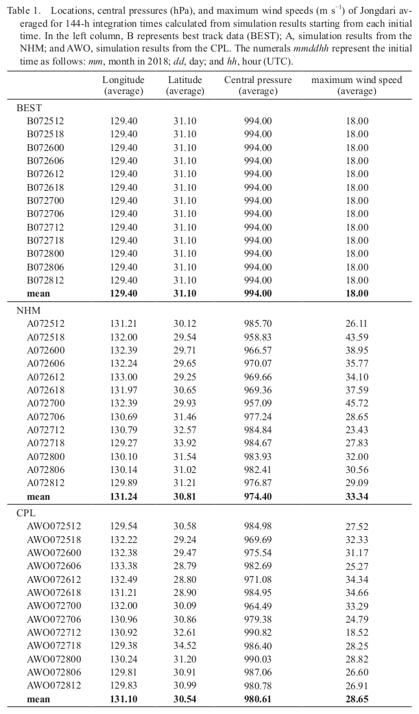
Figure 6 shows the time series of the average diff erences in the track and central pressure between the noncoupled- and coupled-model simulations. CPL reduced the error in the track simulations after 60 h compared with NHM. The simulated intensity was closer to the best track for the noncoupled-model simulations up to 60 h and for the coupled-model simulations after 84 h. The improvement in central pressure simulations in the latter part of the integration time is an expectable effect of ocean coupling (Bender et al. 1993; Ito et al. 2015; Mogensen et al. 2017; Wada et al. 2010, 2018; Wada 2021). The question is how ocean coupling affected the TC vortex itself and the UTCL surrounding the TC. The next section discusses how Jongdari and the UTCL behaved in the simulation results.
3.3 Interaction of the simulated Jongdari with the UTCLThis section presents Jongdari and the UTCL in the noncoupled-model simulations. Figure 7 maps pressure at an altitude of approximately 10 km along with sea-level pressure and Ertel's PV (Davis and Emanuel 1991) (1 PV unit = 10−6 m2 s−1 K kg−1) on the 355-K isotherm surface and shows vertical profiles of PV, potential temperature, and horizontal–vertical wind vectors parallel to the cross section along the line connecting the centers of Jongdari and the UTCL at the integration times of 0, 36, 72, and 108 h after the initial time of 12 UTC on 25 July. It should be noted that the height of 10 km is lower than that of the UTCL (12 km) used in Figs. 3 and 4, although this difference does not affect our conclusions. The horizontal distributions in all cases in this paper are averaged over the neighboring 16-grid cells (approximately 50 km), except the distribution of hourly precipitation.

In the intensification phase (0–36 h), the TC vortex was relatively small (Figs. 7a, b), resembling that of a marginal tropical storm (Molinari et al. 1998) or a midget TC (Lander 1994). However, a tower of positive PV (> 1 PV unit) associated with the TC (hereafter referred to as the PV tower) was clearly depicted extending from the lower to the middle troposphere (Fig. 7c). On the other hand, the UTCL was characterized by low pressure around 10 km and high PV in the upper troposphere (Fig. 7b). As Jongdari moved north–northeastward in the simulation and the UTCL moved southwestward (Figs. 7d, e), southerly winds around the eastern edge of the UTCL strengthened. The simulated TC moved along the northeastern edge of the cyclonic circulation, and the value of PV on the 355-K isotherm surface became small. Jongdari was intensifying in the simulation when the outflow from the PV tower became evident (Fig. 7f).
As the simulated Jongdari moved westward along the Japanese coast (Fig. 7g) and the high-PV area in the UTCL descended in altitude while the UTCL was moving southwestward (Fig. 7h), the PV tower approached the Japanese archipelago (Fig. 7i) and then weakened (Fig. 7l). The high-PV area on the 355-K isotherm surface was stretching and cyclonically folding (Fig. 7h), resembling the deformation of a fluid surface computed by a barotropic model in which the layers behave like a two-dimensional ideal fluid (Welander 1955). In the simulation, Jongdari continued to follow the geostrophic-balanced cyclonic circulation centered at the UTCL, which is one of the factors that affects the steering flow. When Jongdari moved over the Japanese archipelago, the central pressure in the UTCL increased. This indicates that the TC weakened at that time as a result of surface friction on land. Indeed, the PV tower weakened during the passage over land (not shown). When Jongdari moved over the ocean south of Kyushu in the simulation (Fig. 7j), the cyclonic circulation centered at the area within the UTCL shrank in size (Fig. 7k) and the PV tower intensified again. Even though the UTCL became weak, for convenience we continue to refer to it as the UTCL. At 00 UTC on 30 July in the simulation, the tilt of the upper-level high PV (> 1 PV unit) (Agusti-Panareda et al. 2004) or tropopause folding (Price and Vaughan 1993; Bosart 2003) had reversed from its direction at 36 h and 72 h (Fig. 7l), and the location of the TC appeared to be identical to that of the UTCL.
Geostrophic-balanced cyclonic circulation was induced below the UTCL at the initial time (Fig. 8a). As the UTCL moved southwestward at 36 h, the distance between the TC and the UTCL became closer than before, but the geostrophic circulation of Jongdari was still separated from the geostrophic-balanced cyclonic circulation centered within the UTCL (Fig. 8b). The geostrophic flows within the inner core of Jongdari were clearly found in the intensification phase, although, in general, the gradient wind balance is established rather than the geostrophic wind balance within the inner core of a TC (e.g., Miyamoto et al. 2014). At 72 h, geostrophic-balanced cyclonic circulation centered within the UTCL was located in the area centered around 29°N, 136°E (Fig. 8c). The TC moved westward along the northern edge of the UTCL-induced geostrophic-balanced cyclonic circulation. At 108 h, the geostrophic-balanced cyclonic circulation was not clear and became part of the inner-core structure of Jongdari (Fig. 8d). This suggests that the magnitude of the UTCL-induced geostrophic-balanced cyclonic circulation became weak. The gradient winds of the simulated TC may affect the steering flows. The modification of the steering flow due to the excessively simulated gradient winds of Jongdari possibly affect the difference in TC tracks between the simulations and the best track analysis.

Next, we present the thermodynamic conditions of Jongdari and the UTCL in the simulation. Figure 9 maps the horizontal moisture flux (specific humidity multiplied by momentum per unit mass) at an altitude of approximately 10 km, the relative humidity at the height of the 355-K isotherm surface, and the relative humidity along with the potential temperature and horizontal–vertical wind vectors parallel to the cross section along the line between the centers of Jongdari and the UTCL at the integration times of 0, 36, 72, and 108 h after the initial time of 12 UTC on 25 July. Each panel in Fig. 9 is a counterpart to one in Fig. 7. The altitude of the horizontal moisture flux and relative humidity is set to 10 km to clearly show the difference between the dry area at the lower end of the UTCL and the convection area of the TC.

At an altitude of approximately 10 km, the horizontal moisture fluxes were relatively high on the western side of the UTCL and higher than the moisture fluxes around Jongdari at the initial time, 12 UTC on 25 July (Fig. 9a). This high-moisture area corresponds to the area where the relative humidity was higher than 50 % on the 355-K isotherm surface, while the relative humidity at the center of the UTCL was close to zero (Fig. 9b). The area of > 50 % relative humidity was spread zonally around Jongdari. The cross section between Jongdari and the UTCL shows that the tropopause, where the vertical temperature gradient is steeper than that within the troposphere, dropped to an altitude of approximately 12 km around 36°N, 147°E, while the air with relatively high relative humidity (> 70 %) at an altitude of around 8–10 km near 32.5°N, 145°E was carried upward to the upper troposphere (Fig. 9c).
At 36 h integration time, the moisture flux was relatively high in the arc-shaped area from north to east of UTCL (Fig. 9d). High-moisture fluxes around Jongdari were on the southeastern side of the UTCL and joined the arc-shaped area. The area of low relative humidity (< 20 %) stretched horizontally to the southwest and then folded around 30°N, 140°E (Fig. 9e). The shape of the arc of the dry area was opposite to the arc-shaped area of the moisture fluxes. The relative humidity around Jongdari increased on the 355-K isotherm surface during the intensification phase of TC, and the distance between the UTCL and Jongdari decreased (Figs. 4, 9f). The folding of the tropopause around the UTCL was deflected toward Jongdari. Immediately below the area of folding, the relative humidity was locally higher than 70 % around 31°N, 139°E, and at an altitude of 8–10 km.
At 72 h, the moisture flux was highest around Jongdari just before landfall, and relatively high to the north and northwest of the UTCL. On the 355-K isotherm surface, an arc of relatively dry air south of Jongdari formed as the dry area of the UTCL combined with another body of dry air, a slot in the middle-to-upper troposphere that flowed cyclonically from the continent (Fig. 9h). The flow of this dry slot was captured by the atmospheric motion vectors above 350 hPa (Fig. 3). The UTCL gained moisture while it was moving southwestward and the distance between the UTCL and Jongdari further decreased (Figs. 4, 9i). Since the TCs simulated by NHM and CPL are affected by the lateral boundary conditions updated every 6 hours (e.g., Wada 2017), the influence of the dry slot on the interactions between the UTCL and Jongdari may be affected by the setting of the computational domain and the width of the lateral boundary, as explained in Section 2.3. The effect of setting the width of the lateral boundary on the simulation of the dry slot is beyond the scope of this study.
At 108 h, high-moisture flux was confined to an area around Jongdari (Fig. 9j). On the 355-K isotherm surface, an area of > 50 % relative humidity likewise surrounded Jongdari (Fig. 9k), and the area of > 70 % relative humidity around Jongdari had become reduced in altitude from its height at 72 h (Fig. 9l). The UTCL structure was no longer visible in the cross section. During these movements of the UTCL, the dry air within it was gradually humidified and the tropopause around it rose, and it became obscured as it approached and then coalesced with Jongdari.
This humidification process below the UTCL should degrade the capacity of the UTCL to sustain its low pressure and dry condition in the upper troposphere due to increases in specific humidity at an altitude of approximately 10 km from 0.1 g kg−1 at the initial time to 0.6 g kg−1 at 108 h at the center of the UTCL (Fig. 4a). This means that the low pressure of the UTCL was hardly sustained due to the humidification process and thereby increases in specific humidity in the UTCL. The increases in specific humidity (humidification) were considered to be caused by cumulus convection over the warm ocean and its associated diabatic heating since the interaction between the TC and the ocean plays a crucial role in supplying heat and moisture from the ocean to the atmosphere and in transporting the heat and moisture upward by cumulus convection around the TC and the edge of the UTCL. Given that the TC intensity produced by NHM was stronger than the best track TC intensity (Table 1), the following questions arise: how ocean coupling processes affect the interaction between Jongdari and the UTCL and how simulation results can better incorporate ocean coupling.
3.4 Effect of ocean coupling on simulated Jongdari and UTCLSea surface cooling such as that induced by Jongdari along its track, shown in Fig. 2, is mainly caused by vertical turbulent mixing and upwelling in the upper ocean (Price 1981). This fact suggests that CPL or at least the atmosphere–ocean coupled model is required to reflect the dynamic and thermodynamic processes in simulations of Jongdari. An accurate simulation of sea surface cooling requires an accurate atmospheric forcing to be applied to CPL as well as an accurate oceanic initial condition, particularly the stratification in the upper ocean. In addition, CPL needs to simulate surface wind speeds realistically. Here we investigate the results simulated by CPL in detail. The ocean waves simulated by CPL affect the roughness length over the ocean and thereby change the wind stress or frictional velocity between the atmosphere and the ocean as well as the vertical turbulent mixing caused by breaking waves (Wada et al. 2010).
Figure 10 maps the SST simulated by CPL. The SST initial condition at 12 UTC on 25 July successfully matches the observations shown in Fig. 2, an indication that the SST initial condition was well created by interpolations in the simulations. However, the simulated sea surface cooling induced by Jongdari was relatively weak because the simulated intensity of Jongdari was weaker than the best track intensity even when NHM was used (Table 1). The reason why the sea surface cooling was small as the TC moved rapidly westward is that the vertical turbulent mixing beneath the TC had weakened owing to the weakening of the atmospheric forcing.

Figure 11 maps hourly precipitation in simulations by NHM and CPL at the integration times of 36, 72, and 108 h. NHM simulated heavy rainfall around the TC center at 36 h (Fig. 11a), and another area of precipitation was centered around 29°N, 145°E, where the relative humidity on the 355-K isotherm surface was relatively high (see Fig. 9e). As Jongdari approached land at 72 h, its center was an area of heavy rainfall, and narrow spiral rainbands trailed it on its southeastern side (Fig. 11b). At 108 h, a concentric rainfall pattern surrounded Jongdari as the TC redeveloped south of Kyushu (Fig. 11c). The simulation by CPL showed a small effect of ocean coupling on the distribution of hourly precipitation at 36 h (Fig. 11d). At 72 and 108 h, however, the area of heavy precipitation became smaller than in the noncoupledmodel simulations (Figs. 11e, f). The presence of narrow spiral rainbands below the UTCL during the integration reveals that local convection and associated diabatic heating occurred below the UTCL.

Figure 12 maps latent heat fluxes from the ocean to the atmosphere simulated by NHM and CPL at the integration times of 36, 72, and 108 h. The latent heat flux was relatively high around the edge of the cyclonic circulation and exceeded 400 W m−2 around the simulated TC and along the south coast of Japan around 34.5°N, 139°E (Fig. 12a). At 72 h, when the simulated TC approached the Japanese archipelago, the latent heat flux exceeded 400 W m−2 along the south coast of Japan around 34.5°N, 137°E, while the latent heat flux around the edge of cyclonic circulation became smaller than before (Fig. 12b). At 108 h, the area of latent heat flux exceeding 400 W m−2 was clearly found only within the inner core of simulated TC (Fig. 12c). The difference in latent heat fluxes caused by ocean coupling was found within the inner core of the simulated TC at 36 h. The latent heat flux also decreased below the UTCL around 32°N, 139°E, although the amount of the decreases was relatively small compared to that around the TC. The decrease in latent heat fluxes was found not only around the TC but also below the UTCL around 30°N, 135°E (Figs. 12e, f). The area of the decreases in latent heat fluxes extended from the limited TC area to the entire area below the UTCL as the integration time proceeded. Hereinafter, it will be shown that the reduction in latent heat fluxes below the UTCL due to ocean coupling helped suppress the convection and associated diabatic heating there.

Figure 13 corresponds to Fig. 7, except the results simulated by CPL. At 36 h, there was no significant difference between the noncoupled- and coupled-model simulations of the distribution of pressure at an altitude of approximately 10 km or PV on the 355-K isotherm surface (compare between Figs. 13a, b and Figs. 7d, e); however, the effect of ocean coupling appeared in a decrease in the height of the PV tower of Jongdari and its magnitude (compare Fig. 13c and Fig. 7f). In addition, ocean coupling decreased the upper-tropospheric outflow by more than 10 m s−1 oriented from the top of the PV tower at 14–16 km and thus, modified the locations of low-PV areas formed in the upper troposphere.

At 72 h, the pressure at 10 km altitude at the center of the UTCL was lower in the coupled-model simulation (Fig. 13d) than in the noncoupled-model simulation (Fig. 7g). The PV surrounding the UTCL was higher in the coupled-model simulation (Fig. 13e) than in the noncoupled-model simulation (Fig. 7h). The height of the PV tower was shorter in the coupled-model simulation (Fig. 13f) than in the noncoupled-model simulation (Fig. 7i). These differences due to ocean coupling were more apparent at 108 h (compare between Figs. 13g, h and Figs. 7j, k). They caused a delay in the coalescence of the UTCL and Jongdari; in the noncoupled-model simulation, the PV tower extended from the surface to the tropopause (“V” in Fig. 7l) and the tropopause folding tilted away from the PV tower (“T” in Fig. 7l), whereas in the coupled-model simulation (Fig. 13i), the tropopause folding (“V” in Fig. 13i) still tilted toward the PV tower (“T” in Fig. 13i).
Figure 14 shows the difference in geostrophic flows at an altitude of approximately 10 km between the noncoupled- and coupled-model simulations with wind vectors indicating geostrophic flows in the coupled-model simulation. The map of the difference in geostrophic flows at 36 h (Fig. 14a) shows that the magnitude of the geostrophic flows was almost the same as that in the noncoupled-model simulation (Fig. 8b), although the magnitude around the TC was ∼ 25 m s−1 smaller in the coupled-model simulation (Fig. 14a) than that in the noncoupled-model simulation (Fig. 8b). These features were also found at 72 h (Fig. 14b). However, the geostrophic-balanced cyclonic circulation was ∼ 20 m s−1 stronger in the coupledsimulations (Fig. 14b). At 108 h, the difference in geostrophic flows exceeded 20 m s−1 only around the TC (Fig. 14c). Even though the locations of the TC and the UTCL significantly differed between the noncoupled- and coupled-model simulations, particularly at the latter integration time (72 h and 108 h), the UTCL-induced geostrophic-balanced cyclonic circulation was not clearly found east of the simulated TC at 108 h and thus, it is hard to determine the direct impact of ocean coupling on the geostrophic-balanced cyclonic circulation.

Figure 15 corresponds to Fig. 9, except the results simulated by CPL. At 36 h, ocean coupling had produced no significant difference in the maps (compare Figs. 15a–c and Figs. 9d–f) between the noncoupled- and coupled-model simulations, except regarding the area around the PV tower, where relative humidity was relatively high in the noncoupled-model simulation.

At 72 h, the area where moisture flux exceeded 2 g m−2 s−1 at an altitude of 10 km around the circumference of the UTCL (Fig. 15d) was larger than the area in the noncoupled-model simulation (Fig. 9g). The area with less than 10 % relative humidity on the 355-K isotherm surface around the UTCL was smaller (Fig. 15e) than in the noncoupled-model simulation (Figs. 9g, h), but the downward intrusion of dry air from the UTCL toward Jongdari was stronger above an altitude of 12 km in the coupled-model simulation (“X” in Fig. 15f) than that in the noncoupled-model simulation (“X” in Fig. 9i). At 108 h, the moisture flux at an altitude of 10 km near Jongdari was more widespread in the coupled-model simulation (compare Fig. 15g and Fig. 9j). Unlike the result at 72 h (Fig. 15e), an area with < 10 % relative humidity on the 355-K isotherm surface was apparent on the north side of Jongdari (Fig. 15h). In addition, the downward intrusion of dry air from the UTCL toward Jongdari was still apparent (Fig. 15i). Around the PV tower of Jongdari, the area with > 70 % relative humidity was higher than in the noncoupled-model simulation, exceeding an altitude of 10 km (compare Fig. 15i and Fig. 9l). This may partly result from the difference between the noncoupled- and coupled-model simulations in the structure of the PV tower and the nearby low-PV area in the area of upper-tropospheric outflow.
Our results demonstrate that adding ocean coupling to the atmosphere model helps reduce the PV around the PV tower of Jongdari. In addition, ocean coupling helps suppress warming of the air below the UTCL and thereby helps suppress the spread of decreased PV around the UTCL. The reduction due to ocean coupling in hourly precipitation below the UTCL also reduces upper-tropospheric warming around the UTCL through processes such as reduction in latent heat fluxes from the ocean to the atmosphere; weakening convection and associated diabatic heating, particularly around the eyewall of the TC that moved along the circumference of the UTCL; suppressing the production of areas of low PV in the upper troposphere there; and environmental effects that may help maintain high upper-level PV around the UTCL. The reduction in PV around the outflow area of Jongdari reduced upper-troposphere warming around the UTCL, and the strengthened intrusion of dry air from the UTCL to the vicinity of Jongdari due to relatively strong geostrophic-balanced cyclonic circulation were all factors in delaying the coalescence of the UTCL and Jongdari. The delay in the coalescence due to ocean coupling, interacting with the enlarged and strengthened geostrophic-balanced cyclone circulation induced by the relatively strong UTCL, resulted in a difference in the simulated track of Jongdari.
3.5 Initial conditions and predictabilityThe dry areas surrounding both the UTCL and Jongdari included the continental high, the dry slot from the continental high, and another UTCL over the ocean east of Japan (Fig. 3) that appeared at 108 h integration time (Fig. 9k) when the initial time was 12 UTC on 25 July. The atmospheric environments at the initial time and those provided as lateral boundary conditions differ depending on the initial time of integration, influencing the simulated track and intensity of Jongdari. In fact, the simulated location (Fig. 4), intensity (Fig. 5a) and size (Fig. 5b) of Jongdari differed greatly depending on the initial time of integration; the resulting difference in track simulations was much greater than that caused by ocean coupling. In this section we compare the noncoupled-model and coupledmodel simulations under initial conditions based on four different initial times.
Figure 16 shows the distribution of relative humidity and PV on the 355-K isotherm surface and the vertical cross section of PV on the line between the centers of Jongdari and the UTCL based on the JMA data at the four following times: 06, 12, and 18 UTC on 27 July and 00 UTC on 28 July. These were selected as initial times to provide an integration time of less than 72 h before 00 UTC on 30 July, the time at which Jongdari redeveloped south of Kyushu and coalesced with the UTCL (Fig. 7i). An integration time of less than 72 h was chosen to reduce, to some extent, the effect of ocean coupling on the simulations and to focus on the effect of the difference in the atmospheric initial conditions.

At 06 UTC on 27 July, the UTCL with low relative humidity (Fig. 16a) and high PV (Fig. 16b) lay south of Japan. At that time, Jongdari was located southeast of the UTCL. The PV tower of Jongdari and the tropopause folding (> 1 PV unit) from the UTCL lay along the vertical cross section, and they were approximately 500 km apart at an altitude of 8 km (Fig. 16c). At 12 UTC on 27 July, the UTCL had moved southward and Jongdari had moved cyclonically around the circumference of the UTCL compared to their positions 6 h earlier (Figs. 16d, e). The centers of Jongdari and UTCL were less than 500 km apart at an altitude of 10 km (Fig. 16f). At 18 UTC on 27 July, the dry area (Fig. 16g) with high PV was oriented northwest–southeast rather than north–south (Fig. 16h). Although the height of the PV tower was unchanged from the simulation starting 6 h earlier (Fig. 16i), the area with high relative humidity on the 355-K isotherm surface had become concentrated near the center of Jongdari. At 00 UTC on 28 July, Jongdari's motion had changed to west–northwestward while its maximum intensity matched the best track central pressure (Fig. 5). The center of the UTCL coincided with the dry area at the eastern edge of high-PV area, and Jongdari had moved along the circumference of the UTCL (Figs. 16j, k). The PV tower and the tropopause folding extending from the UTCL were approximately 200 km apart at an altitude of approximately 11 km (Fig. 16l). The upward motion was clear from the lower troposphere to the top of the PV tower, and the outflow from the PV tower went to the southeast. In contrast, the winds from the tropospheric folding to the PV tower were northwesterly. Overall, the behavior of the UTCL and Jongdari as analyzed from different atmospheric initial conditions was continuous. It appears unfeasible to detect a difference in the simulations that can be attributed to the atmospheric initial conditions.
Figure 17 shows maps of relative humidity (Fig. 17a) and potential vorticity (Fig. 17b) at the height of the 355-K isotherm surface and the vertical cross section of PV on the line AB shown in Figs. 17a, b (Fig. 17c) based on JMA 6-hourly global atmospheric analysis data at 00 UTC on 30 July. The relative humidity was high west of the TC within the inner core, whereas PV was high east of the TC. The height of the TC tower was approximately 8 km, and the PV in the UTCL was relatively high, from 12 km to 14 km, east of the TC.

Figure 18 corresponds to Fig. 16 except results of simulations by NHM starting at four different initial times (i.e., at integration times of 48, 54, 60, and 66 h). All four simulations featured a relatively dry area east–southeast of Jongdari (Fig. 18a) and high PV on the 355-K isotherm surface (Fig. 18b), although the locations of high-PV area relative to the TC center were different from the global analysis, particularly around the analyzed high-PV area at the height of the 355-K isotherm surface (Fig. 17b). The cross-section line in the noncoupled-model simulation that started at 18 UTC on 27 July (Figs. 18g, h) differed from the others in its orientation owing to the difference in the relative positions of Jongdari and the UTCL due to the track error. In fact, the simulated track that started at 18 UTC on 27 July corresponds to a track passing through Jeju Island in Fig. 4, which is approximately 227 km northwest of the ensemble mean position. The relative positions of the tropopause folding and the PV tower differed with the initial time of the integration (Figs. 18c, f, i, l). The shorter the integration time, the closer the relative position to the analysis distribution. Note that the heights of the PV tower in these four simulations were lower than that in the noncoupled-model simulation with the initial time of 12 UTC on 25 July (Fig. 7l), which implies that the intensity of Jongdari was overestimated in the noncoupled-model simulation with the earlier initial time. However, the heights of the PV tower in all four simulations (Figs. 18c, f, i, l) were still higher (∼ 10 km or higher) than that of the analyzed PV tower (∼ 8 km) (Fig. 17c). This suggests that the coalescence of Jongdari and the UTCL did not actually occur and thus, the coalescence in the noncoupled-model simulation starting at 12 UTC on 25 July was unrealistic.

The results of the coupled-model simulations at the four different initial times (Fig. 19) differed somewhat from those of the noncoupled-model simulations (Fig. 16). The direction of the cross-section line did not change due to ocean coupling, while the line clearly differs among the four atmospheric initial conditions (compare Figs. 18a, d, g, j and Figs. 19a, d, g, j). This indicates that the atmospheric initial conditions determined the arrangement of simulated Jongdari and UTCL and their evolutions. The high-PV area on the 355-K isotherm surface southeast of Jongdari was slightly larger (from 10,000 km2 to 46,000 km2) than that in the noncoupled-model simulations due to ocean coupling (Figs. 19b, e, h, k), except the simulated area that started at 18 UTC on 27 July (Fig. 19h). The location of the high-PV area relative to the TC center in the coupled-model simulations (Figs. 19b, e, h, k) was closer to the location of the analyzed high PV area (Fig. 17b) than those in the noncoupled-model simulations (Figs. 18b, e, h, k). The reduction in the amplitude of positive PV in the PV tower was approximately 1.2 PVU (Fig. 19c), 0.2 PVU (Figs. 19f, i), and 1.4 PVU (Fig. 19l) in the coupled-model simulations compared to those in the noncoupled-model simulations. The height of the simulated PV tower (Figs. 19c, f, I, l) became close to the analyzed PV tower (Fig. 17c) due to the reduction in the amplitude of positive PV in the PV tower caused by ocean coupling.

Although the geostrophic-balanced cyclonic circulation may dominate the TC movement according to the analysis in Fig. 17, the simulated TC intensity was still overdeveloped compared to the best track analysis even in the coupled-model simulations. The excessively strong gradient winds of the overdeveloped TC may be factors that a large loop south of Kyusyu analyzed in the best track data shrank in the noncoupled- and coupled-model simulations.


