Abstract
The present study uses an object-based evaluation metric to examine the precipitation bias over the Maritime Continent in the global cloud-resolving models. We specifically focus on the difference between the models that directly resolve convection and those using convection parameterization. The 40-day hindcast experiments of the DYnamics of the Atmospheric general circulation Modeled On Non-hydrostatic Domain (DYAMOND) intercomparison project are evaluated against the high-resolution satellite rainfall products. The hindcast of the Central Weather Bureau Global Forecast System (CWBGFS) under the DYAMOND protocol is also included. The results indicate that most models simulate insufficient numbers of large precipitation system [object-based precipitation system (OPS), > 370 km in scale], indicating weaker convection organization. The observation indicates that the maximum precipitation within the OPS intensifies with increasing object size. All of the models capture this positive relationship, but most of them overestimate the sensitivity. Most of the models overestimate both the frequency and intensity of small OPS (< 160 km), except for the models with convection parameterization [i.e., CWBGFS, European Centre for Medium-Range Weather Forecasts Integrated Forecasting System (IFS)-9 km]. Although most of the models can reproduce the observed peak time of diurnal precipitation over the land area in the Maritime Continent, the simulated fractional contribution of different sizes of OPS to the total precipitation varies from model to model, and their peak times do not follow the observed ones with delayed peak times as the size of OPS increases from small, mid-size, to large categories. Most of the models reasonably capture the mean diurnal cycle peak time, but only the models with convection parameterization and Model for Prediction Across Scales (MPAS) can represent the diurnal evolution of fractional contribution from different OPSs. The implications of the current results to the upscale processes of the tropical convection systems in the global models are also discussed.
1. Introduction
Moist convection critically influences the transport of heat, moisture, and momentum in the global climate system. In particular, organized convection significantly contributes to tropical rainfall (Houze 2004; Chen et al. 2021; Yuan and Houze 2010), and the occurrence of these organized convective systems is tightly coupled to large-scale circulation from synoptic, intraseasonal, to seasonal time scales (Jian et al. 2021; Hung et al. 2020; Hoskins et al. 2020; Chen et al. 2021). However, general circulation models (GCMs) have been struggling to represent the convective-scale processes (Randall et al. 2003; Arakawa 2004; Stephens et al. 2010). The associated biases make it difficult to clarify the physics involved in the multi-scale interactions between the development of organized convective systems and the evolution of large-scale circulations.
Previous studies have suggested that by increasing the spatial resolution toward convection-permitting scales, the representation of moist convection can potentially be improved (Tomita and Satoh 2004; Satoh et al. 2008). Several global cloud-resolving models (GCRMs) have been developed along with the significant increase in computational power in the recent decade. The DYnamics of the Atmospheric general circulation Modeled On Non-hydrostatic Domains (DYAMOND) is the first GCRM intercomparison project that aims to investigate the interaction between convective systems and the large-scale circulation when convective-scale circulations are explicitly simulated instead of being parameterized (Stevens et al. 2019). The first phase of the DYAMOND consists of 40-day hindcast simulations for a boreal summer (from August 1st to September 10th, 2016). Basic aspects of the general circulation are well captured by the cloud-resolving models, and the distribution of precipitation and cloud fields can be directly compared with the observations (Stevens et al. 2019).
However, biases have also been identified in the DYAMOND simulations. Arnold et al. (2020) have evaluated the simulated diurnal cycle rainfall in one of the DYAMOND models. They concluded that in the high-resolution simulations without parameterized convection, precipitation tends to peak too early, and diurnal amplitudes develop unrealistic small-scale variability over regions dominated by local thermodynamic forcing. Roh et al. (2021) demonstrated large differences in net shortwave radiation at the top of the atmosphere, vertical cloud distribution, and cloud water content among the DYAMOND models. Model-specific biases also exist in the simulated size and structure of tropical cyclones (Judt et al. 2021).
With the advances of the techniques in satellite remote sensing and numerical modeling, we can compare satellite retrievals and model rainfall at a comparable spatial resolution on the order around 10 km, which can resolve the structures of organized convective system. Su et al. (2019) developed an evaluation metric emphasizing the horizontal scale of convective storms. With the snapshots from either observed or modeled rainfall intensity, the contiguous surface grid cells with rainfall above a certain threshold were connected to obtain an object-based precipitation system (OPS). Observed and simulated fractional contribution to total rainfall from small to large convective storms can be compared based on the same statistical metric. The DYAMOND models differ in the choice of representing moist convection. Some of the models use parameterization for either shallow convection or both shallow and deep convection (described in more detail in Section 2.2). Therefore, it is interesting to apply the OPS-based metric to evaluate the simulated tropical storms among the cloud-resolving models and the models with parameterized convection.
In addition, we include the hindcast simulated by the Central Weather Bureau Global Forecast System (CWBGFS, Liou et al. 1997; Su et al. 2019) in this study. The development of the CWBGFS aims to extend from short-term weather forecasts to subseasonal to seasonal (S2S) forecasts (Vitart et al. 2012) in which the interaction between organized convective systems and the large-scale circulation plays a crucial role. Su et al. (2021) demonstrated that the CWBGFS could represent the observed object-based statistics at a horizontal resolution of 15 km with the unified parameterization (UP). The UP is a framework for conventional convection parameterization, which aims to generalize the representation of deep moist convection between the parameterized and the explicitly resolved processes according to the process-dependent convective updraft fraction (Arakawa et al. 2011; Arakawa and Wu 2013; Wu and Arakawa 2014). In their simulations with the UP, the effects of parameterized convection are reduced depending on the fractional area covered by convective updrafts within the grid cell. Distinct convective updrafts and downdrafts were observed along with the development of convective core regions. Within organized convective systems, the local circulation and the variability of precipitation are enhanced compared with the simulations without the UP. Su et al. (2022) further demonstrated that the UP improves the diurnal cycle over the land area in the Maritime Continent. The diurnal cycle over the Maritime Continent plays a crucial role in the variability of convective activity on the intraseasonal time scale in the tropics (i.e., MJO; Hagos et al. 2016; Peatman et al. 2014), but representing the realistic diurnal cycle has been challenging for numerical models (Sato et al. 2009; Neale and Slingo 2003). With the UP, both the diurnal amplitude and peak time become more realistic compared with the simulations with the conventional parameterized convection.
This study aimed to assess the performance of simulating tropical convective systems among GCRMs and the models with parameterized convection. The performance of the simulated precipitation diurnal cycle will also be examined. We apply the OPS-based metric to evaluate the DYAMOND and the CWBGFS hindcast simulations for rainfall over the Maritime Continent [90–155°E, 12°S–10°N] against the satellite observation from the integrated multi-satellite retrievals for global precipitation measurement (GPM-IMERG, Huffman et al. 2019) and the Climate Prediction Center morphing method (CMORPH, Joyce et al. 2004).
The remainder of this paper is organized as follows. Section 2 describes the methodology and datasets for the present study. Section 3 presents the OPS-based statistics over the Maritime Continent. Section 4 provides the discussion and summary.
2. Methodology
2.1 Observation datasets
The GPM-IMERG provides half-hourly precipitation estimates at the spatial resolution of 0.1° from 60°S to 60°N. This data is a combined retrieval based on GPM microwave imager, dual-frequency precipitation radar (DPR), several types of passive microwave (PMW) radiometers, and infrared (IR) data recorded by geosynchronous weather satellites, with calibration by ground-based rain gauges. The CMORPH provides half-hourly precipitation estimates covering the same area at an 8-km spatial resolution. The CMORPH data is based on PMW sensors. Bias in the satellite precipitation estimates is then removed through comparison against Climate Prediction Center daily gauge analysis over land and adjustment against the Global Precipitation Climatology Project merged analysis of pentad precipitation over ocean. Both datasets can be used to examine the life cycle of tropical convective systems and the evolution of strong precipitation events due to their high temporal-spatial resolution. The differences in the OPS-based statistics between the two datasets can roughly represent the observation uncertainty.
2.2 Model outputs
This study evaluates eight members in the data repository of DYAMOND (https://easy.gems.dkrz.de/DYAMOND) and a hindcast simulation of CWBGFS according to the DYAMOND protocol (Stevens et al. 2019). All the models were integrated for 40 days starting from August 1st, 2016. After a 2-day spin-up, only the last 38 days of outputs are evaluated. In the DYAMOND models, the atmospheric state is initialized by the global 9-km meteorological analysis data from the European Centre for Medium-Range Weather Forecasts. The CWBGFS hindcast is initialized by the ERA5 reanalysis data (Hersbach et al. 2020). The DYAMOND members selected in this study are ARPEGE-NH (hereafter ARPNH), ICON, NICAM, UM, FV3, MPAS, and two IFS members with a different spatial resolution (4 km and 9 km, respectively). The CWBGFS is an atmospheric GCM at a spatial resolution of around 15 km. The model uses the spectral method in the horizontal directions and assumes hydrostatic balance in the vertical as far as its dynamic core is concerned. The representation of moist convection in the CWBGFS has been introduced in Section 1. A detailed description of the physics suite in the CWBGFS can be found in the study by Su et al. (2022).
Among the DYAMOND members, ARPNH, ICON, and NICAM explicitly resolve moist convection. UM, FV3, and IFS-4km parameterize the effects of shallow convection. IFS-9km parameterizes both the effects of shallow and deep convection. MPAS uses a scale-aware cumulus parameterization. At 3.8-km horizontal resolution, the cumulus parameterization is barely active, and most of the convection in MPAS is resolved (Judt and Rios-Berrios 2021). In the CWBGFS, the effects of shallow and deep convection are parameterized at a 15-km horizontal resolution, whereas deep convection can be resolved when the convective updraft fraction approaches unity (Su et al. 2021). For more information about the DYAMOND members, please refer to Stevens et al. (2019) and references therein.
The observation datasets and the model outputs are regridded to the same spatial resolution as the CWBGFS. The interpolation was conducted using the area average method with latitude weighting. After the spatial interpolation, hourly averages of precipitation are calculated for the following analysis to have consistent temporal output among the models.
2.3 Object-based precipitation system (OPS)
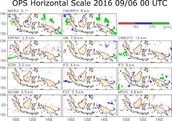
Following Su et al. (2019), contiguous surface grid points where the precipitation rate is stronger than 1 mm h−1 are identified as an OPS representing an organized convective system. The horizontal scale of the OPS is determined by its square root of the area, and we interpret the horizontal scale as a measure of convective organization. We note that a small variation in the precipitation threshold value does not change the major conclusion of the following analyses. The OPSs are classified according to their horizontal scale. The OPSs are classified into three categories based on the IMERG data to evaluate the models: small (< 160 km), mid-size (160–370 km), large (> 370 km). The size dividers of the OPS categories are chosen so that each category of OPSs contributes roughly equal amounts of rainfall in the IMERG data. We note that the object detection for each dataset was carried out after the data interpolation (15 km, hourly). Figure 1 presents an example of the spatial distribution of OPS in a snapshot of each dataset. The native resolution of each dataset is also shown in the figure.
3. Results
3.1 Spatial distribution of OPS occurrence
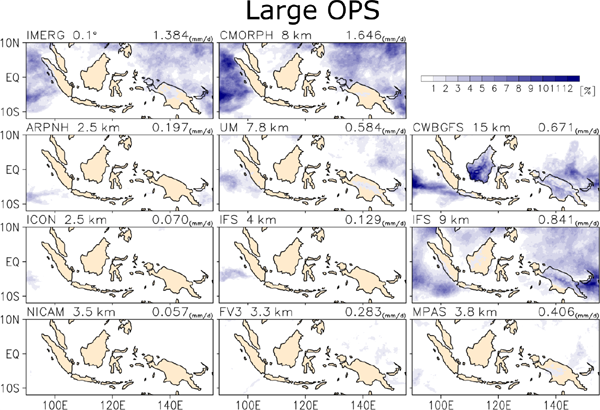
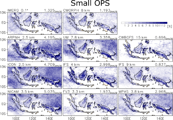
First, we examine the spatial distribution of OPS occurrence over the Maritime Continent region. All the grid points that are part of an OPS are counted in the OPS occurrence frequency. To show the model behavior of the most and the least organized cases, Figs. 2 and 3 present the probability of small and large OPS occurrence over the analysis period, respectively. The top row shows the results from the observational datasets (i.e., IMERG and CMORPH). The rest of the panels demonstrate the results from the DYAMOND models and CWBGFS. The number at the upper-right corner in each panel shows the precipitation intensity contributed by the OPSs averaged over the analysis region [90–155°E, 12°S–10°N]. In Fig. 2, the observations indicate that there are more small OPSs over the islands compared with the surrounding coastal ocean. However, almost all the models overestimate the presence of small OPS over the islands, and several models overestimate the presence of small OPS over the surrounding coastal ocean (i.e., ARPNH, ICON, NICAM, UM, and MPAS). The modeled precipitation contributed by small OPS ranges from 0.70 mm d−1 to 5.04 mm d−1, whereas the observations range from 1.19 mm d−1 to 1.33 mm d−1. Almost all of the models overestimate the small OPS precipitation, except for CWBGFS and IFS-9km, which show an underestimation. We found that the strongest small OPS precipitation was produced by models without any convective parameterization (i.e., ARPNH, ICON, and NICAM). In Fig. 3, the observations indicate that large OPSs occur primarily over the ocean. Most of the models do not simulate sufficient large OPSs, except CWBGFS and IFS-9km. However, CWBGFS overestimates the presence of large OPS over Borneo and New Guinea, and IFS-9km overestimates the presence of large OPS over New Guinea. All of the models underestimate the large OPS precipitation. For example, the large OPS precipitation in ICON and NICAM is less than one-tenth of that in the observations. The result indicates that the models show a large variation in representing convection organization between each other.
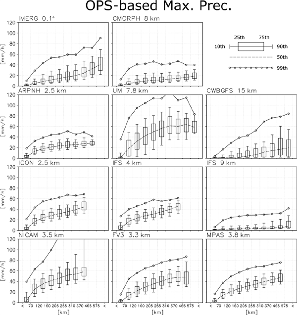
We further examine how the precipitation extreme varies with the OPS horizontal scale over the Maritime Continent in the analysis period. Figure 4 presents the range of the maximum precipitation intensity from the 10th percentile to the 99th percentile for the different horizontal scales of OPS. The x-axis represents the horizontal scales of the OPSs. The bins of the x-axis are determined to assure nearly equal fractional contribution to total rainfall based on the IMERG data. The y-axis shows the precipitation intensity. The observations show increasing 50th and 99th percentiles, and both the interquartile and interdecile range of the maximum precipitation intensities along with the increasing OPS scale. The two observational datasets do show some differences. The CMORPH exhibits weaker precipitation extremes in large convective systems compared with the IMERG. As the IMERG includes the DPR observation, it can detect stronger precipitation intensity than the CMORPH, which is mainly based on PMW. So here, we use the IMERG as the reference when evaluating rainfall extremes. Some of the models overestimate the sensitivity with the OPS scale for the variability of precipitation extremes (i.e., NICAM and UM). A few models underestimate the sensitivity (i.e., ARPNH and IFS-9km). In ARPNH, the interdecile range of the maximum precipitation intensities of large OPSs (> 370 km) is smaller than 20 mm h−1, which is less than half of that in the IMERG. The rest of the models generally fall within the observational difference for this sensitivity. We also examine the sensitivity that the bins of the x-axis are determined according to individual model data (Fig. S1). The results highlight the overestimation of small OPS precipitation in the GCRMs, which is consistent with the results presented in Section 3.1 and the subsequent analysis.
Here, we synthesize the statistics on the phase diagram in Fig. 5. Each dataset is placed according to the number of counts for different scale categories (small, mid-size, and large) along the x-axis in log scale and also according to the fractional contribution to total rainfall for different scale categories along the y-axis. The fractional contribution of all OPS rainfall to the total rainfall of each dataset is also presented in the figure. In the observations, the small (circle) and large (triangle) OPS fractional contributions are comparable with each other, and they are slightly smaller than the mid-size (square) OPS fractional contribution. However, only CWBGFS and IFS-9km capture this relationship (the red symbols in the figure). The other models (the blue symbols) overestimate the contribution from the small OPSs, whereas the number and contribution from the large OPSs are underestimated. Meanwhile, the variability of the fractional contribution of each scale category between these models is large. Although CWBGFS and IFS-9km capture the distribution of fractional contribution for different scale categories of OPS, they and FV3 underestimate the fractional contribution of all OPS rainfall, indicating that the fractional contribution from drizzle (< 1 mm h−1) is larger in these models. For the rest of the models, drizzle occurrence is rarer compared with the observations.

Finally, we examine the diurnal cycle of precipitation over the Maritime Continent. In the 40-day simulations, the large-scale circulation can be diverse between the models, and the convective processes over the land and ocean areas of the Maritime Continent can respond differently to the variation in the large-scale circulation (Rauniyar and Walsh 2011; Peatman et al. 2014). Figure 6 presents the time series of precipitation intensity averaged over the land and oceans area of the Maritime Continent, respectively. The black line shows the mean of the two observational datasets, and the gray lines show the results from the models. Over the land area, the diurnal cycle is the dominant variability in the precipitation time series of both the observations and all the models. The 38-day outputs provide sufficient samples for the diurnal cycle analysis. On the other hand, the observed precipitation time series over the ocean area is dominated by the low-frequency variability, which has a comparable magnitude to the diurnal variability. Outputs from ensemble hindcasts are needed to obtain robust statistics of the variation in the diurnal cycle of precipitation over ocean among the models. Therefore, we will focus on the diurnal cycle over the land area in this study.
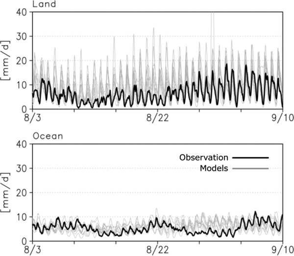
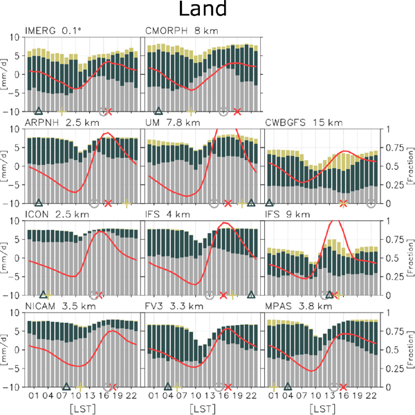
Figure 7 presents the diurnal cycle of precipitation over the land area of the Maritime Continent. The red line indicates the diurnal cycle of average precipitation intensity. The gray, dark gray, and yellow bar demonstrate the fractional contribution to total rainfall from small, mid-size, and large OPS, respectively, at each local hour. The symbols along with the x-axis show the diurnal peak time of each component. We find that the diurnal peak time over the land area in the Maritime Continent is a couple of hours late in the CMORPH compared with the IMERG. Most of the models can accurately simulate the diurnal peak time, but only CWBGFS, MPAS, FV3, and NICAM simulate similar diurnal amplitude as in the observations. The rest of the models overestimate the diurnal amplitude. The observations show that the small OPS contribution increases way before noontime, whereas the mid-size and the large OPSs contribute in the late afternoon to early morning. However, most of the models underestimate the contribution from large OPSs throughout the diurnal cycle, and also, the small OPS contribution is overestimated in these models. Only the models with convection parameterization (i.e., CWBGFS and IFS-9km) and MPAS can represent the diurnal evolution of fractional contribution from different OPSs. In particular, the large OPS contribution in IFS-9km and CWBGFS peaks at the time (yellow plus sign) similar to the diurnal peak time of average precipitation intensity (red cross).
4. Discussion and summary
DYAMOND provides the first opportunity to examine the GCRM performance under the hindcast framework. These models can reasonably capture the overall distribution of precipitation and diurnal cycle evolution over the land area in the Maritime Continent. However, with the object-based statistics, we have found that these models have a very diverse relationship between the spectrum of precipitation extremes and object size and the contribution from the different sizes of the objects to the diurnal precipitation. It is interesting that the models with convection parameterization perform better in some of the metrics, and the models with a finer native resolution are not superior to the others.
Here, we provide an example to demonstrate the variability of convection between a GCRM (NICAM) and a model with parameterized convection (CWBGFS). We first conditionally sample the vertical velocity into a 2° mesh so that the convective behavior can be evaluated over the ascending/descending regions of the large-scale circulation. In NICAM at its original horizontal resolution (Fig. 8a), it is interesting to see that the probability distribution over the descending region (−0.05 m s−1) exhibits large variability with strong convective updrafts/downdrafts. The extreme updrafts and downdrafts (probability of 10−3) become stronger as the large-scale motion increases from −0.03 m s−1. The result indicates that the high-frequency convection in NICAM vigorously develops even over the descending regions of the large-scale circulation. To compare NICAM and CWBGFS, the vertical velocity is regridded into 0.25° mesh and then conditionally sampled by the 2° large-scale motions (Figs. 8b, c). In CWBGFS, the large convection variability mostly occurs over the ascending regions of the large-scale circulation. The extreme updrafts and downdrafts become stronger as the large-scale motion increases from 0.01 m s−1. However, the convection variability with 0.25° mesh is still significant over the descending regions in NICAM. It is found that both the extreme updrafts and downdrafts in NICAM over the ascending regions are twice stronger than those in CWBGFS. Furthermore, these ascending regions in NICAM are distributed more sporadic over the tropical ocean compared with CWBGFS, suggesting that the organization of the high-frequency convection can be the cause of the diverse performance in the relationship between precipitation spectrum and OPS horizontal scale, as presented in Section 3.2. The upscale process of the convection among the models requires further investigation.

Although most of the models perform reasonable diurnal peak time over the land area of the Maritime Continent (Fig. 7), GCRMs generally have too large contribution from small OPSs to total precipitation and overestimate the diurnal amplitude. We found that the bias is consistent with the results from the same diagnostic metric carried out under a coarser resolution (25 km) and a lower criterion of precipitation intensity (0.6 mm h−1) for OPS identification (Fig. S2). In the observation, the contribution to total precipitation from small OPSs peaks first in the early afternoon, followed by mid-size and then large OPSs in the late night. We can reasonably hypothesize that this evolution is associated with the development of organized convective systems. The overestimation of small OPS precipitation in GCRMs may imply that there is a shorter time scale of convective system development. The convective systems dissipate before developing into a more mature stage with a larger horizontal scale. In addition, the representation of topography could play a key role in convective system development. In the future, a convection tracking algorithm (Chang et al. 2021) that identifies the cloud object using 3D hydrometeor fields and links the object snapshots in time will be applied to the DYAMOND model outputs and CWBGFS to evaluate the convection's life cycle, which can be helpful in enhancing the understanding of the multi-scale processes over the Maritime Continent.
To summarize, we use the object-based evaluation on the DYAMOND models and CWBGFS by the size categories of object-based precipitation systems. These GCRMs exhibit significant variations in object-based statistics. The general biases include too many small OPSs, unrealistic dependence of precipitation extremes on OPS scale, insufficient contribution by the large systems, and overestimation of diurnal amplitude over the Maritime Continent land.
Data Availability Statement
The datasets generated and/or analyzed in this study are available from the corresponding author upon reasonable request.
Supplements
Figure S1 presents the spectrum of precipitation extremes (y-axis) for different horizontal scales (x-axis) of OPS as in Fig. 4, but the bins of the x-axis are determined to assure a nearly equal fractional contribution to total rainfall. Figure S2 presents the diurnal variation of average precipitation intensity and the fractional contribution to total rainfall of different scale categories of OPS as in Fig. 7, but the diagnostic metric is carried out under a coarser resolution (25 km) and a lower criterion of precipitation intensity (0.6 mm h−1) for OPS identification.
Acknowledgments
We thank Dr. Christopher Mosley for providing NICAM data. W. Chen is supported by the Ministry of Science and Technology of Taiwan (MOST109-2628-M-002-003-MY3). C. Su and C. Wu are supported by MOST107-2111-M-002-010-MY4 and Academia Sinica (AS-TP-109-M11). H. Ma was funded by the Regional and Global Model Analysis program area and Atmospheric System Research program of the U.S. Department of Energy and his work was performed under the auspices of the U.S. Department of Energy by LLNL under contract DE-AC52-07NA27344. We thank Dr. Jen-Her Chen in Central Weather Bureau for his support of this work.
References
- Arakawa, A., 2004: The cumulus parameterization problem: Past, present, and future. J. Climate, 17, 2493-2525.
- Arakawa, A., and C.-M. Wu, 2013: A unified representation of deep moist convection in numerical modeling of the atmosphere. Part I. J. Atmos. Sci., 70, 1977-1992.
- Arakawa, A., J.-H. Jung, and C.-M. Wu, 2011: Toward unification of the multiscale modeling of the atmosphere. Atmos. Chem. Phys., 11, 3731-3742.
- Arnold, N. P., W. M. Putman, and S. R. Freitas, 2020: Impact of resolution and parameterized convection on the diurnal cycle of precipitation in a global non-hydrostatic model. J. Meteor. Soc. Japan, 98, 1279-1304.
- Chang, Y.-H., W.-T. Chen, C.-M. Wu, C. Moseley, and C.-C. Wu, 2021: Tracking the influence of cloud condensation nuclei on summer diurnal precipitating systems over complex topography in Taiwan. Atmos. Chem. Phys., 21, 16709-16725.
- Chen, P.-J., W.-T. Chen, C.-M. Wu, and T.-S. Yo, 2021: Convective cloud regimes from a classification of object-based CloudSat observations over Asian-Australian monsoon areas. Geophys. Res. Lett., 48, e2021GL092733, doi:10.1029/2021GL092733.
- Hagos, S. M., C. Zhang, Z. Feng, C. D. Burleyson, C. De Mott, B. Kerns, J. J. Benedict, and N. N. Martini, 2016: The impact of the diurnal cycle on the propagation of Madden-Julian Oscillation convection across the Maritime Continent. J. Adv. Model. Earth Syst., 8, 1552-1564.
- Hersbach, H., B. Bell, P. Berrisford, S. Hirahara, A. Horányi, J. Muñoz-Sabater, A. Simmons, C. Soci, S. Abdalla, X. Abellan, G. Balsamo, P. Bechtold, G. Biavati, J. Bidlot, M. Bonavita, G. D. Chiara, P. Dahlgren, D. Dee, M. Diamantakis, R. Dragani, J. Flemming, R. Forbes, M. Fuentes, A. Geer, L. Haimberger, S. Healy, R. J. Hogan, E. Hólm, M. Janisková, S. Keeley, P. Laloyaux, P. Lopez, C. Lupu, G. Radnoti, P. D. Rosnay, I. Rozum, F. Vamborg, S. Villaume, and J.-N. Thépaut, 2020: The ERA5 global reanalysis. Quart. J. Roy. Meteor. Soc., 146, 1999-2049.
- Hoskins, B. J., G.-Y. Yang, and R. M. Fonseca, 2020: The detailed dynamics of the June–August Hadley cell. Quart. J. Roy. Meteor. Soc., 146, 557-575.
- Houze, R. A., Jr., 2004: Mesoscale convective systems. Rev. Geophys., 42, RG4003, doi:10.1029/2004RG000150.
- Huffman, G. J., E. F. Stocker, D. T. Bolvin, E. J. Nelkin, and J. Tan, 2019: GPM IMERG Final Precipitation L3 Half Hourly 0.1 degree x 0.1 degree V06. Goddard Earth Sciences Data and Information Services Center (GES DISC), Greenbelt, MD, doi:10.5067/GPM/IMERG/3B-HH/06.
- Hung, M.-P., W.-T. Chen, C.-M. Wu, P.-J. Chen, and P.-N. Feng, 2020: Intraseasonal vertical cloud regimes based on CloudSat observations over the tropics. Remote Sens., 12, 2273, doi:10.3390/rs12142273.
- Jian, H.-W., W.-T. Chen, P.-J. Chen, C.-M. Wu, and K. L. Rasmussen, 2021: The synoptically-influenced extreme precipitation systems over Asian-Australian monsoon region observed by TRMM Precipitation Radar. J. Meteor. Soc. Japan, 99, 269-285.
- Joyce, R. J., J. E. Janowiak, P. A. Arkin, and P. Xie, 2004: CMORPH: A method that produces global precipitation estimates from passive microwave and infrared data at high spatial and temporal resolution. J. Hydrometeor., 5, 487-503.
- Judt, F., and R. Rios-Berrios, 2021: Resolved convection improves the representation of equatorial waves and tropical rainfall variability in a global nonhydrostatic model. Geophys. Res. Lett., 48, e2021GL093265, doi:10.1029/2021GL093265.
- Judt, F., D. Klocke, R. Rios-Berrios, B. Vanniere, F. Ziemen, F. L. Auger, J. Biercamp, C. Bretherton, X. Chen, P. Düben, C. Hohenegger, M. Khairoutdinov, C. Kodama, L. Kornblueh, S.-J. Lin, M. Nakano, P. Neumann, W. Putman, N. Röber, M. Roberts, M. Satoh, R. Shibuya, B. Stevens, P. L. Vidale, N. Wedi, and L. Zhou, 2021: Tropical cyclones in global storm-resolving models. J. Meteor. Soc. Japan, 99, 579-602.
- Liou, C. S., J. H. Chen, C. T. Terng, F. J. Wang, C. T. Fong, T. E. Rosmond, H. C. Kuo, C. H. Shiao, and M. D. Cheng, 1997: The second–generation global forecast system at the central weather bureau in Taiwan. Wea. Forecasting, 12, 653-663.
- Neale, R., and J. Slingo, 2003: The Maritime Continent and its role in the global climate: A GCM study. J. Climate, 16, 834-848.
- Peatman, S. C., A. J. Matthews, and D. P. Stevens, 2014: Propagation of the Madden–Julian Oscillation through the Maritime Continent and scale interaction with the diurnal cycle of precipitation. Quart. J. Roy. Meteor. Soc., 140, 814-825.
- Randall, D., M. Khairoutdinov, A. Arakawa, and W. Grabowski, 2003: Breaking the cloud parameterization deadlock. Bull. Amer. Meteor. Soc., 84, 1547-1564.
- Rauniyar, S. P., and K. J. E. Walsh, 2011: Scale interaction of the diurnal cycle of rainfall over the Maritime Continent and Australia: Influence of the MJO. J. Climate, 24, 325-348.
- Roh, W., M. Satoh, and C. Hohenegger, 2021: Intercomparison of cloud properties in DYAMOND simulations over the Atlantic Ocean. J. Meteor. Soc. Japan, 99, 1439-1451.
- Sato, T., H. Miura, M. Satoh, Y. N. Takayabu, and Y. Wang, 2009: Diurnal cycle of precipitation in the tropics simulated in a global cloud-resolving model. J. Climate, 22, 4809-4826.
- Satoh, M., T. Matsuno, H. Tomita, H. Miura, T. Nasuno, and S. Iga, 2008: Nonhydrostatic icosahedral atmospheric model (NICAM) for global cloud resolving simulations. J. Comput. Phys., 227, 3486-3514.
- Stephens, G. L., T. L'Ecuyer, R. Forbes, A. Gettelmen, J.-C. Golaz, A. Bodas-Salcedo, K. Suzuki, P. Gabriel, and J. Haynes, 2010: Dreary state of precipitation in global models. J. Geophys. Res., 115, D24211, doi:10.1029/2010JD014532.
- Stevens, B., M. Satoh, L. Auger, J. Biercamp, C. S. Bretherton, X. Chen, P. Düben, F. Judt, M. Khairoutdinov, D. Klocke, C. Kodama, L. Kornblueh, S.-J. Lin, P. Neumann, W. M. Putman, N. Röber, R. Shibuya, B. Vanniere, P. L. Vidale, N. Wedi, and L. Zhou, 2019: DYAMOND: The DYnamics of the Atmospheric general circulation Modeled On Non-hydrostatic Domains. Prog. Earth Planet. Sci., 6, 61, doi:10.1186/s40645-019-0304-z.
- Su, C.-Y., C.-M. Wu, W.-T. Chen, and J.-H. Chen, 2019: Object-based precipitation system bias in grey zone simulation: The 2016 South China Sea Summer Monsoon onset. Climate Dyn., 53, 617-630.
- Su, C.-Y., C.-M. Wu, W.-T. Chen, and J.-H. Chen, 2021: Implementation of the unified representation of deep moist convection in the CWBGFS. Mon. Wea. Rev., 149, 3525-3539.
- Su, C.-Y., C.-M. Wu, W.-T. Chen, and J.-H. Chen, 2022: The effects of the unified parameterization in the CWBGFS: The diurnal cycle of precipitation over land in the Maritime Continent. Climate Dyn., 58, 223-233.
- Tomita, H., and M. Satoh, 2004: A new dynamical framework of nonhydrostatic global model using the icosahedral grid. Fluid Dyn. Res., 34, 357, doi:10.1016/j.fluiddyn.2004.03.003.
- Vitart, F., A. W. Robertson, and D. L. T. Anderson, 2012: Subseasonal to seasonal prediction project: Bridging the gap between weather and climate. WMO Bull., 61, 23-28.
- Wu, C.-M., and A. Arakawa, 2014: A unified representation of deep moist convection in numerical modeling of the atmosphere. Part II. J. Atmos. Sci., 71, 2089-2103.
- Yuan, J., and R. A. Houze, Jr., 2010: Global variability of mesoscale convective system anvil structure from A-Train satellite data. J. Climate, 23, 5864-5888.