Flux Adjustment on Seasonal-Scale Sea Surface Temperature Drift in NICOCO

Abstract

High-resolution atmosphere–ocean coupled models are the primary tool for subseasonal to seasonal-scale (S2S) prediction. However, seasonal-scale sea surface temperature (SST) drift is inevitable due to the imbalance between the model components, which may deteriorate the prediction skill. Here, we investigate the performance of a simple flux adjustment method specifically designed to suppress seasonal-scale SST drift through case studies. The Nonhydrostatic Icosahedral Atmospheric Model (NICAM)–Center for Climate System Research Ocean Component Model (COCO) coupled weather/climate model, referred to as NICOCO, was used for wintertime 40-day integrations with a horizontal resolution of 14 km for the atmosphere and 0.25° for the ocean components. The coupled model with no flux adjustment suffers SST drift of typically −1.5–2°C in 40 days over the tropical, subtropical, and Antarctic regions. Simple flux adjustment was found to sufficiently suppress the SST drift. Nevertheless, the lead–lag correlation analysis revealed that air-sea interactions are likely to be appropriately represented under flux adjustment. Thus, high-resolution coupled models with flux adjustment can significantly improve S2S prediction.

1. Introduction

There is growing demand for the improvement of subseasonal to seasonal-scale (S2S) predictions (White et al. 2022). Successful prediction of extreme events, such as tropical cyclones and heat waves, over the S2S scale is important for disaster prevention and mitigation. Atmosphere and ocean coupled models are argued to be essential for better S2S prediction as ocean conditions can be a major source of predictability on the S2S scale (e.g., Mariotti et al. 2018; Vitart and Robertson 2018). A coupled model outperforms an atmosphere-only model in predicting the intensities of tropical cyclones (Ito et al. 2015). Furthermore, Nakano and Kikuchi (2019) and Fu and Wang (2004) argued that coupled models have better skills than uncoupled atmospheric ones in representing tropical intraseasonal oscillations, namely, the Madden-Julian Oscillation (MJO) (Madden and Julian 1971, 1972) and Boreal Summer Intraseasonal Oscillation (Kikuchi 2021), which are also sources of S2S predictability. Zhu et al. (2018) argued that the prediction skill in MJO is improved by using a sea surface temperature (SST) distribution predicted by a coupled model via a two-tiered approach. Miyakawa et al. (2017) demonstrated that for the MJO event in 1998, a global coupled model exhibited better prediction skill than the corresponding atmosphere-only model. In the S2S Prediction Project Database (Vitart et al. 2017), half of the participating models are operated as an atmosphere and ocean coupled system.

In numerical models, higher horizontal resolution generally leads to better representation of the atmosphere and ocean states by resolving smaller-scale features, including atmospheric convection cells and ocean eddies (e.g., Czaja et al. 2019; Caldwell et al. 2019; Delworth et al. 2012; Roberts et al. 2018; Small et al. 2014). Due to recent advancements in computational performance, the horizontal resolution of global numerical models has rapidly improved. To comprehensively investigate the benefit of improving horizontal resolution, high-resolution atmospheric and atmosphere–ocean coupled models were integrated over 50 years and longer under the protocol of the High-Resolution Model Intercomparison Project (HighResMIP) (Haarsma et al. 2016), where the participating atmospheric and ocean models typically have 50-km and 25-km resolution, respectively. Even higher-resolution model integrations were conducted for shorter integration periods under the initiative of the Dynamics of the Atmospheric General Circulation Modeled on Non-hydrostatic Domains (DYAMOND) Phase II (https://www.esiwace.eu/services/dyamondinitiative), which is the successor of the DYAMOND Phase I project (Stevens et al. 2019).

Thus, high-resolution coupled models are important tools for improving S2S prediction. However, model drift on the seasonal timescale is inevitable due to the imbalance between the components, even with state-of-the-art coupled models, which could deteriorate the prediction skill. As reviewed by Weaver and Hughes (1996), various flux adjustment methods have been proposed to suppress model drifts. Flux adjustment was employed to adjust the equilibrium state in a coupled model for decade-long integration with a horizontal resolution typically coarser than 2° grid spacing (e.g., Cubasch et al. 1992; Manabe et al. 1991). However, to the best of our knowledge, flux adjustment has not been fully tested on seasonal-scale drift in a coupled model with cloud-permitting and eddy-permitting resolutions or even finer.

In this study, we investigated the performance of a simple flux adjustment method to suppress SST drift on a seasonal timescale. Some previous studies warn that flux adjustment may result in an artificially new equilibrium state (e.g., Egger 1997; Rahmstorf, 1995). However, our intention is to achieve realistic seasonal SST evolutions with reasonable air-sea interaction processes maintained, rather than adjusting the equilibrium state for climate sensitivity investigation. With SST evolution that is free from drift, a high-resolution coupled model would yield improved prediction performance for atmospheric and ocean events on the S2S scale, such as MJO or tropical cyclones. To this end, we implemented a simple flux adjustment routine for a high-resolution coupled model as described below. This study investigates its performance through a case study.

2. Data and method

We conducted several sets of atmosphere and ocean coupled global integrations over 40 days with the Nonhydrostatic Icosahedral Atmospheric Model (NICAM)–Center for Climate System Research Ocean Component Model (COCO) coupled weather/climate model (hereafter NICOCO) (Miyakawa et al. 2017; Satoh et al. 2014). The atmospheric component NICAM version 19.1 (Satoh et al. 2014; Tomita et al. 2001), ocean component COCO version 4.9 (Hasumi 2006), and general-purpose coupler Jcup (Arakawa et al. 2011, 2020) were used for the coupled system. The version of NICAM was updated from NICAM.14.2 used in Miyakawa et al. (2017). In this study, the horizontal resolution of NICAM was equivalent to 14 km with 40 vertical levels, and COCO had a nominal 0.25° resolution with 63 vertical levels. The resolutions were higher than the standard resolution in the HighResMIP models.

The detailed model configurations are presented in Tables 1 and 2. COCO was configured to use bi-harmonic Smagorinsky-like viscosity (Griffies and Hallberg 2000), second-order moments conserving scheme for tracer advection (Prather 1986), and turbulent closure scheme formulated by Noh and Kim (1999). Following Kodama et al. (2021), NICAM was configured to use the bulk formula formulated by Louis (1979) for surface fluxes, Mellor–Yamada–Nakanishi–Niino Level 2 turbulent scheme (Nakanishi and Niino 2006; Noda et al. 2010), orographic gravity wave drag scheme (McFarlane 1987), Minimal Advanced Treatments of Surface Interaction and Runoff (MATSIRO) for the land surface parameterization (Takata et al. 2003), and MSTRNX for the radiation (Sekiguchi and Nakajima 2008). The net surface heat, water, and momentum fluxes were estimated in the atmospheric component and passed to the ocean component every 30 min. At the same time, the SST, sea ice concentration, sea ice thickness, snow depth over sea ice, and temperature of sea ice estimated in the ocean component were passed to the atmosphere component. To estimate the flux adjustment amount, we also used COCO as an uncoupled system with the same resolution.

In this study, we chose the boreal midwinter of 2009–2010 as a test case. A list of these experiments is presented in Table 3. The initial condition for the ocean component was obtained by spinning up COCO with the Japanese 55-year atmospheric reanalysis designed for driving ocean–sea ice models (JRA55-do) (Tsujino et al. 2018), starting in 1958 with no-motion, climatological-mean temperature, and salinity obtained from the World Ocean Atlas 2013 (Boyer et al. 2013). To obtain a set of 10 initial atmospheric conditions, the reanalysis products of ERA5 (Hersbach et al. 2020) at 00 UTC were used for each date from December 23, 2009, to January 1, 2010. To mitigate the initial imbalance between NICAM and COCO in the coupled integrations, the uncoupled NICAM was spun up from each of the initial atmospheric conditions until January 5. Throughout the spin-up of NICAM, a fixed SST distribution on January 5, 2010, obtained from the uncoupled COCO spin-up was prescribed. Then, 10 ensemble coupled integrations were conducted over 40 days from January 5 to February 13, 2010, with and without flux adjustment; the details of this method is explained below.

Various flux adjustment methods have been proposed to obtain realistic equilibrium states in a coupled model integration (Egger 1997; Manabe et al. 1991; Sausen et al. 1988), but there is no consensus on the best method. The original idea of flux adjustment is to obtain the equilibrium states of the individual uncoupled components by imposing appropriate amounts of surface fluxes, and anomalies around the equilibrium are predicted by the models (Cubasch et al. 1992; Voss et al. 1998). Because the integration period was relatively short in this study, our intention was to achieve a realistic seasonal SST evolution as the ensemble-mean by adjusting the surface fluxes, rather than adjusting the equilibrium state. In this framework, each ensemble member represents a possible realization that is wobbling around the ensemble-mean seasonal evolution. To minimize artificial intervention, flux adjustment was used only to surface heat fluxes given to the ocean surface; hence, no adjustments were applied to momentum, freshwater, and surface heat fluxes to the atmosphere.

In this study, the flux adjustment amount was designed to adjust the SST evolutions in NICOCO to those in the uncoupled COCO. We used SST from the uncoupled COCO as the reference rather than observation due to the large SST bias of COCO near the western boundary currents, as described in the following section. The large SST bias would lead to unnaturally large adjustment fluxes that could cause numerical instability.

One of the simplest methods for estimating the flux adjustment amount proposed by Weaver and Hughes (1996) and von Storch (2000) was employed. First, an uncoupled COCO was integrated with the JRA55-do forcing from January 5 to February 13, 2010, to obtain daily mean SST (hereafter COCO-SST) and total surface heat fluxes (COCO-THF). Second, a set of 10-member ensemble integrations of uncoupled NICAM was conducted with the daily COCO-SST prescribed for the same period starting with the 10 initial atmospheric conditions described above. Thus, the ensemble-mean of the daily mean total surface heat fluxes (NICAM-THF) was obtained. The flux adjustment amount (hereafter F (x, y, t), where x, y, and t indicate longitude, latitude, and time, respectively) was determined as the difference between COCO-THF and NICAM-THF. Note that the flux adjustment is distinct from the nudging of SST toward a reference state. In the nudging, F is evaluated during the coupled integrations and depends on the atmospheric and oceanic states realized in each integration. Meanwhile, in the flux adjustment, F can be a function of time (t), but F is independent of the atmosphere and ocean realizations in the coupled experiments, and thus, exactly the same among the ensemble members.

This simple method is advantageous as any arbitrary parameters, such as relaxation constants, are unnecessary. Weaver and Hughes (1996) argued that some typical flux adjustment methods, including the one used in the present study, converge to the same flux adjustment amount. Therefore, the results in the following sections are likely to be insensitive to the choice of the method, whereas there may be a better method that requires only a smaller amount of adjustment fluxes (Weaver and Hughes 1996).

To examine the importance of the temporal resolution in F (x, y, t), we conducted two sets of flux-adjusted NICOCO integrations. In one integration, F (x, y, t) is averaged over the analysis period beforehand and added as a temporary constant term while retaining its spatial variation. In the second experiment, F (x, y, t) was updated daily.

3. Results and discussion

3.1 Seasonal-scale SST drift

Figure 1a presents SST differences between the uncoupled COCO and ERA5 on the last day of the integration. The SST product of ERA5 is equivalent to the Operational Sea Surface Temperature and Sea Ice Analysis system (Donlon et al. 2012). Although the differences were negligible over the tropical–subtropical region, COCO had large biases over the midlatitude and Antarctic regions. The large biases over the western boundary of the midlatitude ocean are due to the poleward shift in the western boundary currents, a well-known feature of ocean models with a quarter-degree resolution or coarser (Choi et al. 2002; Nakano et al. 2008). We confirmed that these biases are improved in uncoupled COCO integrations with a resolution of 0.1°, which will be described in a separate paper. The large warm bias in the Antarctic region may be related to the poor representation of sea ice in COCO or biases in the JRA55-do forcing; however, detailed investigations are beyond the scope of this study.

Fig. 1.

SST bias in the uncoupled COCO experiment and SST drift in the NICOCO experiments. (a) A map of bias in daily mean SST based on the uncoupled COCO relative to ERA5 on February 13, 2010 (°C; shaded) and the corresponding SST biases relative to the uncoupled COCO based on (b) NICOCO free experiment, (c) NICOCO with constant flux adjustment, and (d) NICOCO with daily updated flux adjustment. The black boxes indicate target domains for examining the SST time series presented in Fig. 7.

Figures 1b–d present the SST drift in NICOCO on the 40th day. The SST drift is defined as the deviation of ensemble-mean SST in NICOCO from the uncoupled COCO. In the NICOCO experiment without flux adjustment (hereafter NICOCO free experiment), SST exhibits a marked warming drift over the tropical–subtropical region (Fig. 1b). The drift is particularly large along the western coast of South America and Africa as also observed in the other coupled models (Caldwell et al. 2019; Small et al. 2014). Furthermore, the warming drift is prominent along Antarctica and the western coast of Australia.

F (x, y, t) is obtained as the deviation of the total surface heat fluxes in the uncoupled COCO from the ensemble-mean of uncoupled NICAM integrations. Note that the sign convention is positive for downward heat fluxes throughout the study; hence, positive heat fluxes warm the ocean. The total surface heat fluxes are largely positive (negative) over the summer (winter) hemisphere (Fig. 2). The differences (Fig. 2c) indicate that NICAM has positive biases over the tropical–subtropical and Antarctic regions, which is consistent with the warming SST drift. The sign reversal in Fig. 2c corresponds to the F (x, y, t) applied to the NICOCO integration with constant flux adjustment.

Fig. 2.

Total surface heat fluxes averaged over the integration period (W m⁻²; shaded; positive for downward) based on (a) uncoupled COCO, (b) uncoupled NICAM, and (c) their difference (NICAM minus COCO). The contours indicate the SST drift (every 0.5 °C; zero contours are omitted) with the NICOCO free experiment. The gray boxes indicate the target domains for examining the SST time series presented in Fig. 7.

Furthermore, we predicted the distribution of the SST drift based on the total surface heat flux bias by using heat balance equations for the oceanic mixed layer (e.g., Ohishi et al. 2017; Qiu and Kelly 1993), namely,   

Here, T_mix denotes the mixed layer temperature; H, mixed layer depth; Q_net, downward surface net heat flux; and q_sw, downward shortwave radiation at the depth of H. For simplicity, q_sw is assumed to be zero, the density of the seawater ρ₀ is 1026 kg m⁻³, and the specific heat of the seawater C_p is 3900 J K⁻¹ kg⁻¹. The climatological-mean mixed layer depth (de Boyer Montégut 2004) is used for H. For Q_net, the total surface heat flux differences between the ensemble-mean NICAM experiments and the uncoupled COCO experiments, averaged over the integration period, are used. The predicted SST drift (Fig. 3) largely replenishes the SST drift in the NICOCO free experiments (Fig. 1b). Thus, the main factor of the drift is confirmed to be the heat flux bias.

Fig. 3.

The SST drift in the NICOCO free experiment (contoured for every 0.5 °C) and predicted SST drift estimated from the surface total heat flux bias and mean mixed layer depth using Eq. (1) (shaded). The gray boxes indicate the target regions where the time series in Fig. 7 are estimated.

By comparing the uncoupled NICAM outputs with the Japanese ocean flux dataset using remote-sensing observations (J-OFURO3; Tomita et al. 2019), it is observed that the overestimation of incoming solar radiation at the surface in NICAM is the main factor for the drift (Fig. 4). Furthermore, insufficient evaporation, which is manifested as an overestimation of the downward turbulent latent heat flux, is also responsible for the SST drift over the North Pacific subtropical region and along the western coast of Australia. The overestimation of the surface heat fluxes is consistent with the underestimation of cloud cover (Kodama et al. 2021) and surface wind speed (not shown).

Fig. 4.

Maps of deviations in downward (a) total, (b) latent, and (c) shortwave radiation heat fluxes of the ensemble-mean of the uncoupled NICAM experiments from J-OFURO3 averaged over the integration period. The contours indicate the SST drift in the NICOCO free experiment (every 0.5 °C). The gray boxes indicate the target regions where the time series in Fig. 7 are estimated.

Figure 1c presents the SST drift in the NICOCO experiment with constant flux adjustment. The drift is successfully suppressed over most of the global ocean regardless of the simplicity of the method. We confirmed that the drift is suppressed throughout the integration period (not shown) as well as on the 40th day. Although there was still a weak drift of approximately 1 °C over the central tropical Pacific, it was suppressed by updating the F (x, y, t) every day (Fig. 1d).

3.2 Lead–lag correlation

The above results indicated that flux adjustment successfully suppressed the seasonal-scale SST drift. Nevertheless, flux adjustment is desirable to undistort the air–sea interaction process on a shorter timescale. To confirm this, lead–lag correlations between SST and surface turbulent heat fluxes (sensible and latent heat fluxes combined) were investigated. It has been argued that lead–lag profiles illustrate a causal relationship between atmospheric and ocean variability (Bishop et al. 2017; Frankignoul and Hasselmann 1977; Hasselmann 1976; von Storch 2000; Wu et al. 2006). In a situation where atmospheric variations drive SST anomalies, the correlation becomes negative (positive) when SST leads (lags), and the simultaneous correlation is close to zero (note that the sign convention here is positive for downward surface heat fluxes). In the opposite case, where ocean variations drive atmospheric anomalies, the correlation is strongly negative around zero lag, where surface turbulent heat fluxes act as damping for SST perturbations and gradually reduce their amplitude toward larger leads and lags.

Figure 5 presents lead–lag correlations obtained for the three sets of the NICOCO experiments. To remove high-frequency weather noises, 3-day mean time series are composed, and then seasonality is removed. The 10 ensemble members in each set of experiments are pooled together to obtain a single map of correlation (more details in Appendix).

Fig. 5.

Lead–lag correlations between the SST and surface turbulent heat fluxes. Maps of (a) SST leading, (b) simultaneous, and (c) SST lagging correlation between 3-day mean SST and downward sensible and latent heat fluxes combined based on the NICOCO free experiments. The lead or lag is one time step with the 3-day mean time series. Areas with insignificant correlations at 99 % confidence interval are filled in white. (d)–(e) represent maps similar to (a)–(c), respectively, but based on the NICOCO experiments with constant flux adjustment. (g)–(i) represent maps similar to (a)–(c), respectively, but based on the NICOCO experiments with daily updated flux adjustment.

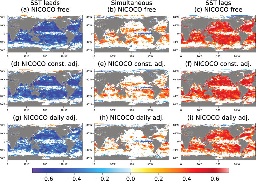
The NICOCO free experiments exhibited a statistically significant negative correlation over the subtropical and higher-latitude domains when SST led (Fig. 5a). The correlation was distinctly weaker at zero lag (Fig. 5b) and became positive when SST lagged (Fig. 5c). The lead–lag pattern implies that SST anomalies are driven by atmospheric processes through surface turbulent heat fluxes. Over the eastern tropical Pacific domain, only the simultaneous positive correlation was significant, indicating that SST variations predominantly modulate the surface turbulent heat fluxes. The lead–lag correlation features were largely consistent with the observations (Fig. 6), except for the northern part of the North Pacific and North Atlantic. Model biases (Wu et al. 2006) and observational errors may be responsible for these discrepancies. However, a detailed investigation was beyond the scope of this study.

Fig. 6.

The same as Fig. 5 but based on (a)–(c) J-OFURO3 and (d)–(f) the uncoupled NICAM experiment.

The correlation patterns in the NICOCO experiments with the constant and daily updated flux adjustment presented in Figs. 5d–f and 5g–i, respectively, are very similar to those in the NICOCO free experiments (Figs. 5a–c). Thus, it is likely that air–sea coupling processes are appropriately represented at timescales of several weeks and shorter under flux adjustment. It is worth pointing out that the correlation features are completely distorted in the uncoupled NICAM experiments (Fig. 6).

A close inspection suggests that NICOCO with daily updated flux adjustment (Figs. 5g–i) exhibits a weaker correlation. Hence, the constant adjustment flux method would be more desirable for better representation of air-sea interaction processes by minimizing artificial intervention, as long as the model drift is satisfactorily suppressed.

4. Seasonal SST evolution

To further elucidate how the flux adjustment specifically suppresses the SST drift, the time evolutions of SST and heat fluxes were examined. Figure 7a presents the time series of SST averaged over the subtropical North Pacific, as indicated by the northern black boxes in Fig. 1, where the constant flux adjustment successfully suppressed the drift. The SST evolution in the uncoupled COCO (black line in Fig. 7a) exhibits linear cooling, which is consistent with the negative total surface heat flux for almost the entire period (black line in Fig. 7b). The NICOCO free experiment (red line in Fig. 7a) also exhibited linear cooling, but the negative slope was insufficient, resulting in a warming drift. In the NICOCO experiments with constant flux adjustment (green line in Fig. 7a), the slope was modified to be more negative due to the negative F (x, y, t), which corresponds to the sign reversal in Fig. 2c. As expected, the SST time series with a daily updated flux adjustment (orange line in Fig. 7a) was almost similar to those of the uncoupled COCO.

Fig. 7.

The time evolutions of SST and heat fluxes over the tropical and subtropical domains. (a) Time series of SST based on the uncoupled COCO (black), NICOCO free (red), NICOCO with constant flux adjustment (green), and NICOCO with daily updated flux adjustment (orange) averaged over [150–180°E, 13–23°N] as indicated by the northern black boxes in Fig. 1. The abscissa indicates the integration time (days) corresponding to January 5 to February 13, 2010. For NICOCO, the thick lines indicate the ensemble means, and the envelopes indicate the maximum and minimum values among the ensemble members. (b) The corresponding downward total heat fluxes based on the uncoupled COCO integrations (black) and ensemble-mean of the uncoupled NICAM integrations (purple) and their difference (orange; COCO minus NICAM). (c) and (d) represent graphs with similar descriptions as (a) and (b), respectively, but averaged over [175°E–155°W, 15°S–5°N].

Within the tropical domain (southern black boxes in Fig. 1), the SST evolution in the uncoupled COCO was nonlinear; SST warmed up slightly until the 16th day and changed to steep linear cooling (black line in Fig. 7c). The time evolution of SST is consistent with the rapid decrease in total heat fluxes in the latter half of the integration (black line in Fig. 7d) and reflects the reduction in the downward shortwave radiation (not shown). The time evolution is consistent with MJO propagation, as defined by the bimodal tropical intraseasonal oscillation index defined by Kikuchi (2021). The time series and corresponding anomaly patterns of the outgoing longwave radiation are available online (http://iprc.soest.hawaii.edu/users/kazuyosh/Bimodal_ISO.html). In the first half of the integration, the target region was in an inactive phase of atmospheric convection due to the negative phase of the MJO and then changed to an active convection phase.

Although the NICOCO free experiment exhibited a steady warning throughout the integration (red line in Fig. 7c), the SST evolution was modified to be nearly constant by the constant flux adjustment (green line in Fig. 7c). The ensemble-mean SST of the NICOCO experiments with daily updated flux adjustment (orange line in Fig. 7c) was similar to that of the uncoupled COCO, as the heat flux adjustment exhibits a rapid decrease to be strongly negative (orange line in Fig. 7d).

Thus, simple flux adjustment has been demonstrated to successfully achieve complicated seasonal SST evolution by frequently updating F (x, y, t). It is worth noting that the two flux-adjusted NICOCO experiments (i.e., constant and daily updated flux adjustment integrations) yield different ensemble-mean SST on the 40th day, despite the fact that the total F (x, y, t) accumulated over the analysis period is exactly the same by definition. We speculated that seasonal variations in oceanic mixed layer depth alter the sensitivity of the mixed layer temperature to surface heat fluxes. This needs to be investigated further in a future study.

5. Summary and conclusion

In this study, we investigated the performance of a simple flux adjustment method for suppressing seasonal-scale SST drift in a global coupled model. We aimed to achieve realistic seasonal-scale evolution in SST to improve S2S prediction skills for extreme events, such as tropical cyclones and heat waves, with a high-resolution coupled system.

Seasonal-scale SST drift was found to be sufficiently suppressed over most of the global ocean by adjusting the heat fluxes applied to the ocean surface; for the other fluxes, no adjustment was required. When flux adjustment is applied to an operational seasonal-scale forecast, F (x, y, t) is estimated in advance from the climatological-mean surface heat fluxes based on an uncoupled ocean model and atmospheric model.

As indicated by the lead–lag correlation, air–sea coupling processes under flux adjustment are likely to be consistent with those in the no flux adjustment experiments. Nevertheless, it should be specifically examined how flux adjustment modifies the representation of atmospheric and oceanic events, such as MJO or tropical cyclones. Given that the lead–lag correlations are somewhat weaker when the flux adjustment amount is frequently updated, it is desirable that the updating intervals are set to be longer than the typical timescale of an event being investigated, as long as the SST drift is sufficiently suppressed.

This paper focuses on the boreal winter of 2009–2010. Nevertheless, we have repeated the same experiments for additional five winters (from 2010–2011 to 2014–2015) to confirm the validity of the method. The simple adjustment method was found to successfully mitigate the SST drift in the five winters; thus, the method is likely to be effective in the other cases. Nevertheless, more detailed evaluation would be required, such as seasonality and quantification of the performance, which would be addressed in future work. Furthermore, we are conducting higher-resolution coupled model simulations, where the atmospheric model has a 3.5-km horizontal resolution, and the ocean model has a 0.1° resolution. The higher-resolution coupled model with flux adjustment will exhibit improved predictions on the S2S timescale.

Data Availability Statement

J-OFURO3 data were downloaded from DIAS (https://doi.org/10.20783/DIAS.612). ERA5 data were downloaded from the Climate Data Store (https://doi.org/10.24381/cds.adbb2d47). The oceanic mixed layer depth was downloaded from the French Research Institute for Exploration of the Sea (https://cerweb.ifremer.fr/deboyer/mld/Surface_Mixed_Layer_Depth.php).

Acknowledgments

We would like to thank the editor and two anonymous reviewers for their constructive suggestions. We thank Drs. Chihiro Kodama and Masao Kurogi for their valuable suggestions. We also thank Drs. Yohei Yamada, Hidetaka Kobayashi, and Takashi Obase for their technical support. This work was supported by MEXT (JPMXP1020200305) as “Program for Promoting Researches on the Supercomputer ‘Fugaku’” (Large Ensemble Atmospheric and Environmental Prediction for Disaster Prevention and Mitigation) and used computational resources of Supercomputer Fugaku provided by the RIKEN Center for Computational Science (ID:hp200128, hp210166, hp220167). J-OFURO3 was obtained from the Data Integration and Analysis System (DIAS), which was developed and operated by a project supported by MEXT. We thank Editage for English language editing.

Appendix

This Appendix describes how the lead–lag correlation between SST and surface turbulent heat fluxes (surface sensible and latent heat fluxes combined) discussed in Section 3 was estimated. The outputs of the first 5 days of the NICOCO and NICAM experiments were discarded to minimize the influence of the initial imbalance. Furthermore, a 3-day mean time series without overlapping was composed to reduce daily weather noise. Thus, 11 time samples of the 3-day mean fields were recorded for each experiment conducted during the 33 days from January 10 to February 11, 2010. To remove seasonality, the least-squares fitting and first harmonic of the Fourier component were removed from the 3-day mean time series. We confirmed that the results were largely insensitive to the deseasonalization methods.

Then, all 10 ensemble members were pooled for each experiment to obtain a single horizontal map of the correlation coefficients. Thus, there were 110 time samples at individual locations for simultaneous correlation and 100 time samples for one lead or lag correlation. Statistical significance was evaluated via t-test at the 99 % confidence interval.

We obtained the corresponding correlation coefficients based on J-OFURO3, a data product of surface heat fluxes and SST obtained from satellite observations and partly atmospheric reanalysis data (Tomita et al. 2019). The daily mean SST and surface heat fluxes were available with some missing data. First, their 3-day mean time series were constructed from January 10 to February 11 with a 10-year period centered on 2010 (i.e., 2006–2015). A 3-day mean value at a particular location and date is considered valid when one of the observations in the corresponding 3-day window is valid; otherwise, it is filled with a horizontal interpolation from the surrounding 3-day mean values. Seasonality was removed, and correlation coefficients were estimated in the same manner as in the NICOCO experiments.

References

•  Arakawa,  T.,  H.  Yoshimura,  F.  Saito, and  K.  Ogochi, 2011: Data exchange algorithm and software design of KAKUSHIN coupler Jcup. Procedia Comput. Sci., 4, 1516–1525.
•  Arakawa,  T.,  T.  Inoue,  H.  Yashiro, and  M.  Satoh, 2020: Coupling library Jcup3: Its philosophy and application. Prog. Earth Planet. Sci., 7, 6, doi:10.1186/s40645-019-0320-z.
•  Bishop,  S. P.,  R. J.  Small,  F. O.  Bryan, and  R. A.  Tomas, 2017: Scale dependence of midlatitude air–sea interaction. J. Climate, 30, 8207–8221.
•  Boyer,  T. P.,  J. I.  Antonov,  O. K.  Baranova,  C.  Coleman,  H. E.  Garcia,  A.  Grodsky,  D. R.  Johnson,  R. A.  Locarnini,  A. V.  Mishonov,  T. D.  O'Brien,  C. R.  Paver,  J. R.  Reagan,  D.  Seidov,  I. V.  Smolyar, and  M. M.  Zweng, 2013: World Ocean Database 2013. NOAA Atlas NESDIS 72, U.S. Department of Commerce, National Oceanic and Atmospheric Administration, National Environmental Satellite, Data, and Information Service, National Oceanographic Data Center, Ocean Climate Laboratory, 208 pp. [Available at https://doi.org/10.7289/V5NZ85MT.]
•  Caldwell,  P. M.,  A.  Mametjanov,  Q.  Tang,  L. P.  Van Roekel,  J.-C.  Golaz,  W.  Lin,  D. C.  Bader,  N. D.  Keen,  Y.  Feng,  R.  Jacob,  M. E.  Maltrud,  A. F.  Roberts,  M. A.  Taylor,  M.  Veneziani,  H.  Wang,  J. D.  Wolfe,  K.  Balaguru,  P.  Cameron-Smith,  L.  Dong,  S. A.  Klein,  L. R.  Leung,  H.-Y.  Li,  Q.  Li,  X.  Liu,  R. B.  Neale,  M.  Pinheiro,  Y.  Qian,  P. A.  Ullrich,  S.  Xie,  Y.  Yang,  Y.  Zhang,  K.  Zhang, and  T.  Zhou, 2019: The DOE E3SM coupled model Version 1: Description and results at high resolution. J. Adv. Model. Earth Syst., 11, 4095–4146.
•  Choi,  B.-H.,  D.-H.  Kim, and  J.-W.  Kim, 2002: Regional responses of climate in the northwestern Pacific Ocean to gradual global warming for a CO₂ quadrupling. J. Meteor. Soc. Japan, 80, 1427–1442.
•  Cubasch,  U.,  K.  Hasselmann,  H.  Höck,  E.  Maier-Reimer,  U.  Mikolajewicz,  B. D.  Santer, and  R.  Sausen, 1992: Time-dependent greenhouse warming computations with a coupled ocean-atmosphere model. Climate Dyn., 8, 55–69.
•  Czaja,  A.,  C.  Frankignoul,  S.  Minobe, and  B.  Vannière, 2019: Simulating the midlatitude atmospheric circulation: What might we gain from high-resolution modeling of air-sea interactions?. Curr. Climate Change Rep., 5, 390–406.
•  de Boyer Montégut,  C.,  G.  Madec,  A. S.  Fischer,  A.  Lazar, and  D.  Iudicone, 2004: Mixed layer depth over the global ocean: An examination of profile data and a profile-based climatology. J. Geophys. Res., 109, C12003, doi:10.1029/2004jc002378.
•  Delworth,  T. L.,  A.  Rosati,  W.  Anderson,  A. J.  Adcroft,  V.  Balaji,  R.  Benson,  K.  Dixon,  S. M.  Griffies,  H.-C.  Lee,  R. C.  Pacanowski,  G. A.  Vecchi,  A. T.  Wittenberg,  F.  Zeng, and  R.  Zhang, 2012: Simulated climate and climate change in the GFDL CM2.5 high-resolution coupled climate model. J. Climate, 25, 2755–2781.
•  Donlon,  C. J.,  M.  Martin,  J.  Stark,  J.  Roberts-Jones,  E.  Fiedler, and  W.  Wimmer, 2012: The Operational Sea Surface Temperature and Sea Ice Analysis (OSTIA) system. Remote Sens. Environ., 116, 140–158.
•  Egger,  J., 1997: Flux correction: Tests with a simple ocean-atmosphere model. Climate Dyn., 13, 285–292.
•  Frankignoul,  C., and  K.  Hasselmann, 1977: Stochastic climate models, Part II Application to sea-surface temperature anomalies and thermocline variability. Tellus, 29, 289–305.
•  Fu,  X., and  B.  Wang, 2004: Differences of boreal summer intraseasonal oscillations simulated in an atmosphere–ocean coupled model and an atmosphere-only model. J. Climate, 17, 1263–1271.
•  Griffies,  S. M., and  R. W.  Hallberg, 2000: Biharmonic friction with a Smagorinsky-like viscosity for use in large-scale eddy-permitting ocean models. Mon. Wea. Rev., 128, 2935–2946.
•  Haarsma,  R. J.,  M. J.  Roberts,  P. L.  Vidale,  C. A.  Senior,  A.  Bellucci,  Q.  Bao,  P.  Chang,  S.  Corti,  N. S.  Fučkar,  V.  Guemas,  J.  von Hardenberg,  W.  Hazeleger,  C.  Kodama,  T.  Koenigk,  L. R.  Leung,  J.  Lu,  J.-J.  Luo,  J.  Mao,  M. S.  Mizielinski,  R.  Mizuta,  P.  Nobre,  M.  Satoh,  E.  Scoccimarro,  T.  Semmler,  J.  Small, and  J.-S.  von Storch, 2016: High resolution model intercomparison project (HighResMIP v1.0) for CMIP6. Geosci. Model Dev., 9, 4185–4208.
•  Hasselmann,  K., 1976: Stochastic climate models. Part I. Theory. Tellus, 28, 473–485.
•  Hasumi,  H., 2006: CCSR ocean component model (COCO) version 4.0. Atmosphere and Ocean Research Institute, The University of Tokyo, 111 pp. [Available at https://ccsr.aori.u-tokyo.ac.jp/~hasumi/COCO/coco4.pdf.]
•  Hersbach,  H.,  B.  Bell,  P.  Berrisford,  S.  Hirahara,  A.  Horányi,  J.  Muñoz-Sabater,  J.  Nicolas,  C.  Peubey,  R.  Radu,  D.  Schepers,  A.  Simmons,  C.  Soci,  S.  Abdalla,  X.  Abellan,  G.  Balsamo,  P.  Bechtold,  G.  Biavati,  J.  Bidlot,  M.  Bonavita,  G.  De Chiara,  P.  Dahlgren,  D.  Dee,  M.  Diamantakis,  R.  Dragani,  J.  Flemming,  R.  Forbes,  M.  Fuentes,  A.  Geer,  L.  Haimberger,  S.  Healy,  R. J.  Hogan,  E.  Hólm,  M.  Janisková,  S.  Keeley,  P.  Laloyaux,  P.  Lopez,  C.  Lupu,  G.  Radnoti,  P.  de Rosnay,  I.  Rozum,  F.  Vamborg,  S.  Villaume, and  J.-N.  Thépaut, 2020: The ERA5 global reanalysis. Quart. J. Roy. Meteor. Soc., 146, 1999–2049.
•  Ito,  K.,  T.  Kuroda,  K.  Saito, and  A.  Wada, 2015: Forecasting a large number of tropical cyclone intensities around Japan using a high-resolution atmosphere–ocean coupled model. Wea. Forecasting, 30, 793–808.
•  Kikuchi,  K., 2021: The boreal summer intraseasonal oscillation (BSISO): A review. J. Meteor. Soc. Japan, 99, 933–972.
•  Kodama,  C.,  T.  Ohno,  T.  Seiki,  H.  Yashiro,  A. T.  Noda,  M.  Nakano,  Y.  Yamada,  W.  Roh,  M.  Satoh,  T.  Nitta,  D.  Goto,  H.  Miura,  T.  Nasuno,  T.  Miyakawa,  Y.-W.  Chen, and  M.  Sugi, 2021: The Nonhydrostatic ICosahedral Atmospheric Model for CMIP6 HighResMIP simulations (NICAM16-S): Experimental design, model description, and impacts of model updates. Geosci. Model Dev., 14, 795–820.
•  Louis,  J.-F., 1979: A parametric model of vertical eddy fluxes in the atmosphere. Bound.-Layer Meteor., 17, 187–202.
•  Madden,  R. A., and  P. R.  Julian, 1971: Detection of a 40–50 day oscillation in the zonal wind in the tropical Pacific. J. Atmos. Sci., 28, 702–708.
•  Madden,  R. A., and  P. R.  Julian, 1972: Description of global-scale circulation cells in the tropics with a 40–50 day period. J. Atmos. Sci., 29, 1109–1123.
•  Manabe,  S.,  R. J.  Stouffer,  M. J.  Spelman, and  K.  Bryan, 1991: Transient responses of a coupled ocean-atmosphere model to gradual changes of atmospheric CO₂. Part I. Annual mean response. J. Climate, 4, 785–818.
•  Mariotti,  A.,  P. M.  Ruti, and  M.  Rixen, 2018: Progress in subseasonal to seasonal prediction through a joint weather and climate community effort. npj Climate Atmos. Sci., 1, 4, doi:10.1038/s41612-018-0014-z.
•  McFarlane,  N. A., 1987: The effect of orographically excited gravity wave drag on the general circulation of the lower stratosphere and troposphere. J. Atmos. Sci., 44, 1775–1800.
•  Miyakawa,  T.,  H.  Yashiro,  T.  Suzuki,  H.  Tatebe, and  M.  Satoh, 2017: A Madden-Julian Oscillation event remotely accelerates ocean upwelling to abruptly terminate the 1997/1998 super El Niño. Geophys. Res. Lett., 44, 9489–9495.
•  Nakanishi,  M., and  H.  Niino, 2006: An improved Mellor–Yamada level-3 model: Its numerical stability and application to a regional prediction of advection fog. Bound.-Layer Meteor., 119, 397–407.
•  Nakano,  H.,  H.  Tsujino, and  R.  Furue, 2008: The Kuroshio Current System as a jet and twin “relative”recirculation gyres embedded in the Sverdrup circulation. Dyn. Atmos. Oceans, 45, 135–164.
•  Nakano,  M., and  K.  Kikuchi, 2019: Seasonality of intraseasonal variability in global climate models. Geophys. Res. Lett., 46, 4441–4449.
•  Noda,  A. T.,  K.  Oouchi,  M.  Satoh,  H.  Tomita,  S.  Iga, and  Y.  Tsushima, 2010: Importance of the subgrid-scale turbulent moist process: Cloud distribution in global cloud-resolving simulations. Atmos. Res., 96, 208–217.
•  Noh,  Y., and  H. J.  Kim, 1999: Simulations of temperature and turbulence structure of the oceanic boundary layer with the improved near-surface process. J. Geophys Res., 104, 15621–15634.
•  Ohishi,  S.,  T.  Tozuka, and  M. F.  Cronin, 2017: Frontogenesis in the Agulhas Return Current region simulated by a high-resolution CGCM. J. Phys. Oceanogr., 47, 2691–2710.
•  Prather,  M. J., 1986: Numerical advection by conservation of second-order moments. J. Geophys. Res., 91, 6671–6681.
•  Qiu,  B., and  K. A.  Kelly, 1993: Upper-ocean heat balance in the Kuroshio Extension region. J. Phys. Oceanogr., 23, 2027–2041.
•  Rahmstorf,  S., 1995: Climate drift in an ocean model coupled to a simple, perfectly matched atmosphere. Climate Dyn., 11, 447–458.
•  Roberts,  M. J.,  P. L.  Vidale,  C.  Senior,  H. T.  Hewitt,  C.  Bates,  S.  Berthou,  P.  Chang,  H. M.  Christensen,  S.  Danilov,  M.-E.  Demory,  S. M.  Griffies,  R.  Haarsma,  T.  Jung,  G.  Martin,  S.  Minobe,  T.  Ringler,  M.  Satoh,  R.  Schiemann,  E.  Scoccimarro,  G.  Stephens, and  M. F.  Wehner, 2018: The benefits of global high resolution for climate simulation: Process understanding and the enabling of stakeholder decisions at the regional scale. Bull. Amer. Meteor. Soc., 99, 2341–2359.
•  Satoh,  M.,  H.  Tomita,  H.  Yashiro,  H.  Miura,  C.  Kodama,  T.  Seiki,  A. T.  Noda,  Y.  Yamada,  D.  Goto,  M.  Sawada,  T.  Miyoshi,  Y.  Niwa,  M.  Hara,  T.  Ohno,  S.  Iga,  T.  Arakawa,  T.  Inoue, and  H.  Kubokawa, 2014: The non-hydrostatic icosahedral atmospheric model: Description and development. Prog. Earth Planet. Sci., 1, 18, doi:10.1186/s40645-014-0018-1.
•  Sausen,  R.,  K.  Barthel, and  K.  Hasselmann, 1988: Coupled ocean-atmosphere models with flux correction. Climate Dyn., 2, 145–163.
•  Sekiguchi,  M., and  T.  Nakajima, 2008: A k-distribution-based radiation code and its computational optimization for an atmospheric general circulation model. J. Quant. Spectrosc. Radiat. Transfer, 109, 2779–2793.
•  Small,  R. J.,  J.  Bacmeister,  D.  Bailey,  A.  Baker,  S.  Bishop,  F.  Bryan,  J.  Caron,  J.  Dennis,  P.  Gent,  H-m.  Hsu,  M.  Jochum,  D.  Lawrence,  E.  Muñoz,  P.  diNezio,  T.  Scheitlin,  R.  Tomas,  J.  Tribbia,  Y.-h.  Tseng, and  M.  Vertenstein, 2014: A new synoptic scale resolving global climate simulation using the Community Earth System Model. J. Adv. Model. Earth Syst., 6, 1065–1094.
•  Stevens,  B.,  M.  Satoh,  L.  Auger,  J.  Biercamp,  C. S.  Bretherton,  X.  Chen,  P.  Düben,  F.  Judt,  M.  Khairoutdinov,  D.  Klocke,  C.  Kodama,  L.  Kornblueh,  S.-J.  Lin,  P.  Neumann,  W. M.  Putman,  N.  Röber,  R.  Shibuya,  B.  Vanniere,  P. L.  Vidale,  N.  Wedi, and  L.  Zhou, 2019: DYAMOND: The DYnamics of the Atmospheric general circulation Modeled On Non-hydrostatic Domains. Prog. Earth Planet. Sci., 6, 61, doi:10.1186/s40645-019-0304-z.
•  Takata,  K.,  S.  Emori, and  T.  Watanabe, 2003: Development of the minimal advanced treatments of surface interaction and runoff. Global Planet. Change, 38, 209–222.
•  Tomita,  H., 2008: New microphysical schemes with five and six categories by diagnostic generation of cloud ice. J. Meteor. Soc. Japan, 86A, 121–142.
•  Tomita,  H.,  M.  Tsugawa,  M.  Satoh, and  K.  Goto, 2001: Shallow water model on a modified icosahedral geodesic grid by using spring dynamics. J. Comput. Phys., 174, 579–613.
•  Tomita,  H.,  T.  Hihara,  S.  Kako,  M.  Kubota, and  K.  Kutsuwada, 2019: An introduction to J-OFURO3, a third-generation Japanese ocean flux data set using remote-sensing observations. J. Oceanogr., 75, 171–194.
•  Tsujino,  H.,  S.  Urakawa,  H.  Nakano,  R. J.  Small,  W. M.  Kim,  S. G.  Yeager,  G.  Danabasoglu,  T.  Suzuki,  J. L.  Bamber,  M.  Bentsen,  C. W.  Böning,  A.  Bozec,  E. P.  Chassignet,  E.  Curchitser,  F. B.  Dias,  P. J.  Durack,  S. M.  Griffies,  Y.  Harada,  M.  Ilicak,  S. A.  Josey,  C.  Kobayashi,  S.  Kobayashi,  Y.  Komuro,  W. G.  Large,  J. L.  Sommer,  S. J.  Marsland,  S.  Masina,  M.  Scheinert,  H.  Tomita,  M.  Valdivieso, and  D.  Yamazaki, 2018: JRA-55 based surface dataset for driving ocean–sea-ice models (JRA55-do). Ocean Modell., 130, 79–139.
•  Vitart,  F., and  A. W.  Robertson, 2018: The sub-seasonal to seasonal prediction project (S2S) and the prediction of extreme events. npj Climate Atmos. Sci., 1, 3, doi:10.1038/s41612-018-0013-0.
•  Vitart,  F.,  C.  Ardilouze,  A.  Bonet,  A.  Brookshaw,  M.  Chen,  C.  Codorean,  M.  Déqué,  L.  Ferranti,  E.  Fucile,  M.  Fuentes,  H.  Hendon,  J.  Hodgson,  H.-S.  Kang,  A.  Kumar,  H.  Lin,  G.  Liu,  X.  Liu,  P.  Malguzzi,  I.  Mallas,  M.  Manoussakis,  D.  Mastrangelo,  C.  MacLachlan,  P.  McLean,  A.  Minami,  R.  Mladek,  T.  Nakazawa,  S.  Najm,  Y.  Nie,  M.  Rixen,  A. W.  Robertson,  P.  Ruti,  C.  Sun,  Y.  Takaya,  M.  Tolstykh,  F.  Venuti,  D.  Waliser,  S.  Woolnough,  T.  Wu,  D.-J.  Won,  H.  Xiao,  R.  Zaripov, and  L.  Zhang, 2017: The Subseasonal to Seasonal (S2S) Prediction project database. Bull. Amer. Meteor. Soc., 98, 163–173.
•  von Storch,  J.-S, 2000: Signatures of air–sea interactions in a coupled atmosphere–ocean GCM. J. Climate, 13, 3361–3379.
•  Voss,  R.,  R.  Sausen, and  U.  Cubasch, 1998: Periodically synchronously coupled integrations with the atmosphere–ocean general circulation model ECHAM3/LSG. Climate Dyn., 14, 249–266.
•  Weaver,  A. J., and  T. M. C.  Hughes, 1996: On the incompatibility of ocean and atmosphere models and the need for flux adjustments. Climate Dyn., 12, 141–170.
•  White,  C. J.,  D. I. V.  Domeisen,  N.  Acharya,  E. A.  Adefisan,  M. L.  Anderson,  S.  Aura,  A. A.  Balogun,  D.  Bertram,  S.  Bluhm,  D. J.  Brayshaw,  J.  Browell,  D.  Büeler,  A.  Charlton-Perez,  X.  Chourio,  I.  Christel,  C. A. S.  Coelho,  M. J.  DeFlorio,  L. D.  Monache,  F. D.  Giuseppe,  A. M.  García-Solórzano,  P. B.  Gibson,  L.  Goddard,  C. G.  Romero,  R. J.  Graham,  R. M.  Graham,  C. M.  Grams,  A.  Halford,  W. T. K.  Huang,  K.  Jensen,  M.  Kilavi,  K. A.  Lawal,  R. W.  Lee,  D.  MacLeod,  A.  Manrique-Suñén,  E. S. P. R.  Martin,  C. J.  Maxwell,  W. J.  Merryfield,  Á. G.  Muñoz,  E.  Olaniyan,  G.  Otieno,  J. A.  Oyedepo,  L.  Palma,  I. G.  Pechlivanidis,  D.  Pons,  F. M.  Ralph,  D. S.  Reis, Jr.,  T. A.  Remenyi,  J. S.  Risbey,  D. J. C.  Robertson,  A. W.  Robertson,  S.  Smith,  A.  Soret,  T.  Sun,  M. C.  Todd,  C. R.  Tozer,  F. C.  Vasconcelos, Jr.,  I.  Vigo,  D. E.  Waliser,  F.  Wetterhall, and  R. G.  Wilson, 2022: Advances in the application and utility of subseasonal-to-seasonal predictions. Bull. Amer. Meteor. Soc., 103, E1448–E1472.
•  Wu,  R.,  B. P.  Kirtman, and  K.  Pegion, 2006: Local air–sea relationship in observations and model simulations. J. Climate, 19, 4914–4932.
•  Zhu,  Y.,  X.  Zhou,  W.  Li,  D.  Hou,  C.  Melhauser,  E.  Sinsky,  M.  Peña,  B.  Fu,  H.  Guan,  W.  Kolczynski,  R.  Wobus, and  V.  Tallapragada, 2018: Toward the improvement of subseasonal prediction in the national centers for environmental prediction global ensemble forecast system. J. Geophys. Res.: Atmos., 123, 6732–6745.