Abstract
A tornado hit Nobeoka city on the southeast coast of Kyushu Island, Japan on 22 September 2019 when Typhoon Tapah was located about 500 km to the southwest of Kyushu Island and moving northeastward. Triply-nested numerical simulations are performed to reproduce the typhoon, a parent storm, and associated tornadoes. The simulation with the coarsest resolution reasonably reproduces Typhoon Tapah and associated outer rainbands at several 500 km east of its center, where the environment around the rainband is found to be favorable for mini-supercells. The simulation with the finest resolution reproduces a train of mini-supercells and associated tornadoes. The mini-supercells have typical structures that cause tornadoes associated with tropical cyclones. The minimum central pressure of the strongest tornado is 945 hPa. The time evolution of the simulated tornadoes is very fast: significant transitions of vortex structure occur within 1 minute before the tornado attains its peak strength. Most of the circulation of the tornado is derived from rear-flank downdrafts. Three tornadoes occur sequentially in association with non-occluding mesocyclogenesis, where a new tornado develops in the northwest of the old one.
1. Introduction
A large fraction of tornadoes in the central United States are spawned by “classic” supercells associated with extratropical cyclones (e.g., Davies-Jones et al. 2001). On the contrary, only a small fraction of tornadoes are spawned by tropical cyclones (Edwards 2012). On the other hand, statistical studies show that a larger fraction of tornadoes (more than 20 %) occurred in association with tropical cyclones in Japan (Niino et al. 1997) and in China (Bai et al. 2020). Typical environments of outer rainbands of tropical cyclones have significant vertical shear at lower altitudes and weaker thermal buoyancy than those of classic supercells. These storms that spawn tornadoes associated with tropical cyclones have smaller sizes in both horizontal and vertical directions (e.g., McCaul 1991; Suzuki et al. 2000): they are referred to as “mini-supercells,” which are specific to the environment of tropical cyclones (e.g., Agee 2014). Tornadoes are likely to occur in the right-front quadrant of tropical cyclones, where the storm-relative helicity (SREH) and the entraining convective available potential energy (E-CAPE) are expected to be large (Sueki and Niino 2016; Bai et al. 2020).
During five years between 2017 and 2021, five strong tornadoes occurred in Japan: one was rated as the Japanese Enhanced Fujita Scale 3 (JEF-3) by the Japan Meteorological Agency (JMA) and the rest as JEF-2. Four out of the five strong tornadoes were associated with tropical cyclones. Thus, tornadoes associated with tropical cyclones are arguably one of the main causes of extreme winds in Japan. Here, we focus on Nobeoka city tornado on 22 September 2019, one of the four strong tornadoes associated with tropical cyclones between 2017 and 2021. Typhoon Tapah in 2019 (Typhoon 1917: the 17th Typhoon in 2019) moved northeastward over the East China Sea in the west of Kyushu Island, Japan (Fig. 1), while it caused serious damage in the east coastal area of the island. A tornado spawned in one of the outer rainbands hit Nobeoka city at 0800 JST (Japan Standard Time; +0900 UTC) on 22 September 2019 (Miyazaki Local Meteorological Observatory 2020), when Typhoon Tapah was already in the mature stage and started to weaken (Fig. 1a). According to the best track data of JMA, the central pressure of Typhoon Tapah was 970 hPa at that time.
The tornado classified as JEF-2 caused 18 injuries and damaged 509 houses (Miyazaki Local Meteorological Observatory 2020). Photographs of funnel clouds taken by several cameras to monitor the water level of rivers in the city showed that it passed over a flat area of Nobeoka city between 0830 JST and 0845 JST on 22 September 2019. A damage survey by the Miyazaki Local Meteorological Observatory showed that the footprints of the tornado started from the southern coast and disappeared in the mountainous area to the north (Fig. 1b). The reflectivity map of the JMA operational radar shows that the tornado was spawned by a storm in one of the outer rainbands of Typhoon Tapah (Fig. 2a), where the storm moved northward toward Nobeoka city (Fig. 2b). However, since the area shown in Fig. 2b is relatively far from the operational radars of JMA, it is difficult to examine detailed characteristics of the tornadic storm using only observational data.
In the absence of detailed observations, a numerical simulation can be a useful approach to understanding the dynamics and structure of the parent storm and associated tornado. A pioneering numerical study of the F2 tornado that hit Nobeoka city on 17 September, 2006 in association with Typhoon Shanshan (Typhoon 0613), whose central pressure at the time of the tornado occurrence was 950 hPa, was performed by Mashiko et al. (2009). The situation in their study was quite similar to that of the present study: tornadoes occurred in an outer rainband in the right-front quadrant of the northward-moving typhoon whose center was located over the East China Sea. However, the damage caused by the tornadoes that hit Nobeoka city in 2006 was more severe. Mashiko et al. (2009) have made a detailed analysis of the source of vorticity and circulation in a simulated tornado and suggested that horizontal vorticity in the strong low-level vertical shear was the source of the rotation of the tornado.
Tornadogenesis is caused by very subtle processes in parent storms (e.g., Coffer et al. 2017; Coffer and Parker 2017; Yokota et al. 2018) and is very complicated because different processes can take place even in a single tornado (Fischer and Dahl 2022). It is of interest to conduct detailed analyses of tornadogensis in the present mini-supercell case and to clarify the similarities and differences with the Typhoon Shanshan case.
The remainder of this paper is organized as follows. Section 2 describes the settings of the numerical simulations. Section 3 presents the mesoscale environment of the tornado examined by the results of the coarse resolution simulation. Section 4 presents the results of a finer resolution simulation which reproduces mini-supercells and associated mesocyclones and tornadoes. Section 5 discusses detailed structures and temporal evolution of tornadoes and mesocyclones in the mini-supercells, and Section 6 gives conclusions.
2. Numerical simulation
The present study uses JMA-NHM (Saito et al. 2006, 2007), a former operational regional weather prediction model of Japan Meteorological Agency based on a non-hydrostatic fully-compressible equation system. It has been used to study various mesoscale and microscale phenomena including real cases of tornadoes, with a very fine resolution (Mashiko et al. 2009; Mashiko 2016a; Yokota et al. 2018; Mashiko and Niino 2017; Tochimoto et al. 2019b; Tochimoto and Niino 2022).
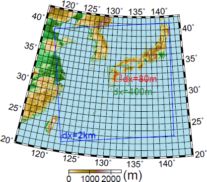
The settings of the numerical model are similar to the previous studies described above. The present study employs triply-nested one-way simulations. Note that Mashiko et al. (2009) used quadruply-nested one-way simulations to study the tornado associated with Typhoon Shanshan in 2006. The horizontal grid spacing dx for the outer, intermediate, and inner domains are set at 2 km, 400 m, and 80 m, respectively, where the corresponding experiments will be hereafter referred to as NHM2km, NHM400m, and NHM80m, respectively. The computational domains of the experiments are shown in Fig. 3. NHM2km uses the topography of GTOPO30 (Global 30 arc-second elevation), while NHM400m and NHM80m use detailed topography (Fig. 1b) and land surface by smoothing the 50 m mesh map provided by the Geospatial Information Authority of Japan. Table 1 shows the configuration of each experiment. The turbulence parameterization is based on Deardorff (1980). A three-ice single-moment bulk scheme (Lin et al. 1983; modified by Ikawa and Saito 1991) is used for microphysics parameterization. Surface fluxes are parameterized as Beljaars and Holtslag (1991).


The calculation domain for NHM2km is large enough to cover the entire Typhoon Tapah (Fig. 3). The initial and boundary conditions for NHM2km are provided by the JMA’s meso-scale analysis (MANL). MANL has spatial and temporal resolution of 5 km and 3 hours, respectively. Therefore, MANL at 0600 JST on 22 September 2019 is used as the initial values, and MANL at 0600 JST and 0900 JST are temporally interpolated to obtain the boundary values for NHM2km. Note that the resolution of MANL has been improved since the time when Mashiko et al. (2009) used it to simulate the tornado. NHM400m was started at 0700 JST and was calculated for 2 hours with initial and boundary values given by the output of NHM2km every 5 minutes. It aimed to reproduce the outer rainband in the east of Typhoon Tapah. Note that the calculation domain for NHM400m does not include the typhoon center. NHM80m was started at 0730 JST and computed for 80 minutes with initial and boundary values given by the output of NHM400m every 5 minutes. The calculation domain of NHM80m is small, but it is sufficient to cover the entire tracks of tornadic vortices.
3. Simulated typhoon and storm environment
NHM2km reasonably reproduced the track and intensity of Typhoon Tapah of the JMA’s best-track data (Fig. 1a). The minimum surface pressure of the simulated Typhoon Tapah is ∼ 970 hPa at the initial time and varies little during the time integration, which is consistent with the best track data. After a spin-up, several outer rainbands developed at about 130, 132, and 134°E at 30°N in the east of its center as shown in Fig. 4, which plots the mixing ratio of precipitating substances, Qp ≡ Qr + Qs + Qg, where Qr, Qs, and Qg are the mixing ratio of rain, snow, and graupel, respectively. The positions of the outer rainbands at 130°E and 132°E agree well with the observations (Fig. 2).

A vertical cross-section across the center of Typhoon Tapah and the rainbands along 31°N is shown in Fig. 5. The precipitation associated with outer rainbands at 130°E and 132°E are separated from the eyewall at 127°E and have a horizontal scale of ∼ 10 km. Its structure is significantly asymmetric, since Typhoon Tapah was in the early phase of an extratropical transition. The wall clouds with slantwise updraft penetrating to the troposphere are evident only on the east side of Typhoon Tapah. Sueki and Niino (2016) showed that tornadic tropical cyclones tend to occur in the early phase of extratropical transitions.

The environmental factors related to tornadogenesis (e.g., Sueki and Niino 2016) are examined (Fig. 6). Sueki and Niino (2016) and Tochimoto et al. (2019a) suggested that convective available potential energy (CAPE) considering the effects of entrainment (entraining CAPE: E-CAPE) is a better indicator of tornado potential. Here, E-CAPE is estimated by assuming an entrainment rate of 20 % km−1. E-CAPE is large near the center of Typhoon Tapah and its outer rainbands, including the one located off the coast of Nobeoka city (Fig. 6a).

Storm-relative environmental helicity (SREH) integrated between the surface and 3 km height with the storm motion estimated from Bunkers et al. (2000) is large near the center of Typhoon Tapah and near the outer rainband off the coast of Nobeoka city (Fig. 6b). Entraining Energy Helicity Index (E-EHI) defined by a product of E-CAPE and SREH with a relevant normalization, which is useful for detecting a potential of a supercell (Tochimoto et al. 2019a), is greater than 10.0 off the east coast of Kyushu Island (Fig. 6c), suggesting that a relatively high potential for supercells.
The simulation with the intermediate resolution, NHM400m, resolves individual storm cells in the rainbands: regions of high mixing ratio of rain water corresponding to these storms moving northward as in the radar observation are reproduced. The hodograph of the environmental wind around the rainband simulated in NHM400m is shown in Fig. 7. SREH for this hodograph is 450 m2 s−1, where the storm motion is estimated to be about 19 m s−1 toward the north. The shape of the hodograph is similar to that in the environment of the Nobeoka tornado associated with Typhoon Shanshan on 17 September 2006 (Fig. 4a in Mashiko et al. 2009), although its SREH between 0 and 3 km was about 700 m2 s−1 and was much stronger than that for the present case.
4. Simulated tornadoes
4.1 Occurrences of three tornadoes and mesocyclones
In NHM80m, three tornadoes are produced, where a tornado is defined as a vortex having vertical vorticity greater than ∼ 0.3 s−1. Figure 8 shows the time series of the maximums of vertical vorticity and horizontal wind speeds, and minima of sea level pressure (SLP) at z = 10 m in the calculation domain. Vertical vorticity maxima of 0.9, 1.5, and 1.0 s−1 occur at about 0755, 0811, and 0830 JST, respectively (Fig. 8a), which will be referred to as tornadoes T1, T2, and T3, respectively. Each tornado has a lifetime of ∼ 10 minutes. The minimum SLP of tornado T2, 945 hPa, in its mature stage (0811:40 JST; Fig. 8b) is lower than that of the simulated tornado associated with Typhoon Shanshan using a similar horizontal resolution (∼ 970 hPa, Mashiko et al. 2009), although SREH is higher in the latter environments. However, since the horizontal grid interval of 80 m is not sufficient to resolve a detailed structure of an actual tornado vortex, it should be noted that the size and vorticity of the simulated vortex need to be taken with some reservation.

The locations of the maximum vertical vorticity in the numerical domain for every 10 seconds are shown in Fig. 9a. These locations almost correspond to the southern end of the rainband, which consists of several cells moving northward off the east coast of Nobeoka (Supplementary Movie S1). Tornado T3 approaches Nobeoka, but does not make landfall and passes through several kilometers offshore. Note, however, that the observed tornado was accompanied by the second southernmost cell in the rainband (Fig. 2). When the vertical vorticity of the tornadic vortices in the rainband becomes weak, the maximum vorticity in the calculation domain is often found near the cape in the southeast of Nobeoka city (Fig. 9a) and is not associated with the tornadoes; the maximum wind speed in the calculation domain is at most 30 m s−1 due to the horizontal roll structures that prevail in the boundary layer (see Appendix). To obtain the track of the tornadoes, another plot is made to show the maximum vertical vorticity in the area excluding the cape (Fig. 9b). Although the rainband moves continuously northward, there are two discontinuities in the tracks of the maximum vertical vorticity. In fact, three distinct tornadic vertical vortices occur in the same rainband.

At 0811:40 JST when tornado T2 is close to its maximum strength, the horizontal wind speed and vertical vorticity of tornado T2 become greater than 50 m s−1 and 0.3 s−1, respectively, within a radius of several 100 m (Figs. 10a, b, e). The flow structures around tornado T2 (Figs. 10b – d) are similar to those of typical classic supercells (e.g., Browning 1964; Lemon and Doswell 1979). The region with large rain water mixing ratio Qr shows a hook-shaped distribution (Fig. 10d).

The horizontal winds in the tornado are significantly asymmetric in both the x and y-directions: the surface winds are stronger on the southeast side of the tornado. The near-surface converging flows into the tornado also cause the asymmetry in the y-direction: they almost cancel the environmental horizontal winds and form a stagnant region along the forward-flank gust front (FFGF) in the north of the tornado (Fig. 10b). On the contrary, the wind speed is enhanced near the rear-flank gust front (RFGF). In this instance, FFGF and RFGF are characterized by isentropes of 299.5 K and 300 K near the surface, respectively (Fig. 10c). The higher potential temperature is found in the center of the tornado (Fig. 10f), suggesting adiabatic heating by a downdraft in the core.
Figure 11 shows the vertical structures along a zonal-vertical cross-section through the center of tornado T2 (x ∼ 62 km). The top of the region with larger mixing ratio of precipitating substances (Qp > 6 g kg−1) reaches only z ∼ 6 km. Strong updrafts exceeding 20 m s−1 occur below z = 6 km at x ∼ 62 km and 64 km (Fig. 11b). The strong updraft at x ∼ 62 km near the surface is associated with tornado T2. Another distinct cell is present between x ∼ 63 km and 66 km: this is reminiscent of an older cell that spawned tornado T1.

The vertical structure of the cell that spawns tornado T2 is similar to those observed for mini-supercells accompanied by tropical cyclones (e.g., Fig. 13 in Suzuki et al. 2000; Fig. 4 in Morotomi et al. 2020). Vault structures are found at the top of these strong updrafts as seen in the region of relatively smaller Qp at x ∼ 61.5 km and z ∼ 3 km (Fig. 11a). A strong downdraft is present in the core of tornado T2, indicating that it has a two-celled structure at this time. Below z = 2 km, the large Qp ∼ 6 g kg−1 is associated with rear-frank downdraft (RFD) at x ∼ 60 km to the west of tornado T2 (Fig. 11). The accumulated precipitation exceeds 40 mm after the passage of the mini-supercell below the hook-shaped region of high Qp (not shown). The near-surface westerly winds that reach tornado T2 originate in the area of RFD where the region of the high Qp reaches the surface at x ∼ 60 km (Figs. 10c, 11a).


Each tornado is accompanied by a mesocyclone with significant positive vertical vorticity. Figure 12 shows the vertical structure of the mesocyclone associated with tornado T2. The horizontal scales of the mesocyclones are ∼ 1 km (Figs. 12a, b), which is less than several km for those of mesocyclones associated with classic supercells (e.g., Lemon and Doswell 1979). At the mature stage of tornado T2, the vertical vorticity of the mesocyclones is an order of magnitude greater than its standard criterion, 0.01 s−1. The centers of the mesocyclones at z = 1 km and 2 km are not right above the tornado but about 500 m and 1 km to the west of the tornado, respectively (Figs. 12a, b). This is consistent with the fact that the updraft and downdraft of the tornado tilt westward with increasing height in the zonal cross-section (Fig. 11). Figure S2 suggests that tornadoes at other times also tend to tilt northwestward with increasing height, although they are upright between the surface and z = 500 m. This tilt of a vertical vortex has also been suggested by an observation of a tornado in a mini-supercell associated with Typhoon Hagibis in 2019 (Adachi and Mashiko 2020).
4.2 Temporal variations of tornado proximity
Figure 13 shows time-height cross-sections of the maximum and minimum vertical velocities and maximum vertical vorticity in the vicinity of the tornadic storm. Above z = 500 m, intensified positive vertical velocity is seen to propagate upward roughly at its own vertical velocity, suggesting the intermittent occurrence of strong updraft plumes in clouds (Fig. 13a). After the strongest tornado T2 occurs near the surface, the downdrafts are also significantly enhanced below the height of z = 4 km (Fig. 13b). The regions of significant vertical vorticity also spread upward with the updrafts (Fig. 13c). However, all significant updrafts are not necessarily accompanied by strong downdrafts (Fig. 13b) nor large vertical vorticity (Fig. 13c). Meanwhile, the heights of the significant updrafts gradually descend before tornadogenesis (Fig. 13a).
Now, the relationships between tornadic vortices near the surface and aloft (i.e., tornadoes and mesocyclones) are examined. Figure 14 shows the footprints of the top 3 strongest vertical vortices at z = 2 km, 1 km, and 20 m. Near the surface (at z = 20 m), only the tracks of the tornadic vortices, which are identical to those in Fig. 9b, are prominent (Fig. 14c). On the other hand, multiple vertical vortices, corresponding to mesocyclones, with comparable magnitudes coexist at the higher altitudes (Figs. 14a, b). They all move northward in the same mini-supercell.

Near the discontinuities in the tracks of tornadic vortices (Fig. 9b), the old tornado gradually weakens and the new tornado develops rapidly to the northwest. At z = 1 km, nearly parallel tracks of two strong vortices can be seen between the latitudes of 32.14°N and 32.22°N and 32.39°N and 32.48°N (Fig. 14b). These vortices move northward at similar speeds, while the west one is located more northward as indicated by the isochrones (purple dotted lines in Fig. 14b). The eastern vortex tends to weaken, whereas the western one tends to strengthen before the replacements of the tornadoes occur near the surface.
Tracks at higher latitudes (z = 2 km) are more variable (Fig. 14a). Strong vertical vortices at z ∼ 2 km are seen in the further south of the mesocyclone at z = 1 km between 32.04°N and 32.14°N and 32.30°N and 32.39°N.
The above results suggest the following scenario of tornadogenesis: mesocyclones at z = 2 km (in the case of a typical classic supercell, at z ∼ 5 km) are first formed; some of them are followed by intensification of mesocyclones at lower altitudes (e.g., z = 1 km), and they eventually produce a tornado near the surface. When the mesocyclone weakens or becomes vertically decoupled from the tornado due to environmental shear near the surface, the tornado weakens. Although a new tornado develops to the east of an old tornado in a typical cyclic tornadogenesis (e.g., Dowell and Bluestein 2002), it develops to the northwest of the old tornado in the present case. The detailed mechanism of this curious cyclic tornadogenesis is discussed in Section 5.4.
5. Discussion
5.1 Evolution of tornado T2 toward its peak strength
The structure of tornado T2 changes significantly within 1 minute before it reaches its peak strength at 0811:40 JST. Figures 15 and 16 show the time evolution of the axisymmetric structures of tornado T2 for every 20 s, where the axisymmetric structure was obtained by averaging the grid point values tangentially.

At 1 minute before the peak strength of T2 (0810:40 JST), the radial flows are directed toward the core below the cloud base (z < 600 m; Figs. 15c, 16c). The tangential wind speed, ut, has a maximum exceeding 25 m s−1 below z < 100 m at r ∼ 200 m (Fig. 15b). Another maximum of ut, exists at the higher altitude, z ∼ 700 m for r > 600 m. The latter maximum corresponds to the lower part of the mesocyclone. The pressure drop in the center at this time is ∼ 10 hPa (Fig. 16c). The updraft is accelerated from the surface to z ∼ 700 m, which is the height of the lower part of the mesocyclone (Fig. 15a).
At 40 s before the peak strength (0811:00 JST), ut near the center of tornado T2 starts to exceed 30 m s−1 (Fig. 15e). The maximum ut near the surface is located between r = 100 m and 200 m. Isolines of the angular momentum M ≡ rut for 20000 m2 s−1 shift about 50 m inward below z ∼ 800 m (Fig. 16d) due to the strong radial inflow (Fig. 15f). The surface pressure and temperature at the core of T2 decrease by 15 hPa and 1 K, respectively (Figs. 16c, f). The updraft becomes weaker (Fig. 15d), possibly due to the decrease in the upward non-hydrostatic vertical pressure gradient at the center.
At 20 s before the peak strength (0811:20 JST), ut is further intensified to be more than 45 m s−1 below z = 100 m (Fig. 15h). The isolines of M except for the innermost one (M = 10000 m2 s−1) in the inflow layer (z ≤ 400 m) shift further inward (Fig. 16g). The updraft at the center weakens but is still more than 5 m s−1 (Fig. 15g). A new maximum of w appears above the maximum of ut, and the outflow is intensified above the maximum of w (Fig. 15i). The surface pressure at the center drops rapidly to ∼ 960 hPa (Fig. 16i). The temperature at the center is 2 K lower than that of the environment due to adiabatic cooling associated with the radial inflow near the surface (Fig. 16h). This cooling leads to the touchdown of the funnel cloud (Fig. 16i).
At the peak strength (0811:40 JST), ut is further intensified to be greater than 50 m s−1 (Fig. 15k). The depth of the inflow layer becomes shallower than 200 m, and the radial flow ur exceeds 25 m s−1 near the center (Fig. 15l). Not only the tangential but also the radial flow contribute considerably to the maximum horizontal wind speed of tornado T2, which is ≥ 80 m s−1 (Fig. 8c). The downdraft exceeding −10 m s−1 occurs in the center (Fig. 15j), due to the downward non-hydrostatic pressure gradient near the surface (Fig. 16l). The water vapor transports by strong updrafts near the center of tornado T2 also affect the cloud formation associated with the tornado: the lower atmosphere is intrinsically humid over the sea; the water vapor mixing ratio increases locally along the updrafts (Figs. 16h, k). Thus, it contributes in part to the formation of the funnel cloud (Figs. 16i, l).
Previous laboratory experiments have shown that the swirl ratio is critical for the morphology of a tornado-like vortex (e.g., Church et al. 1979): the downdraft in the center reaches closer to the surface with increasing the swirl ratio. In the present case, the inflow (ur) rather than the rotation (ut ) increases more significantly as the tornado approaches the peak strength (Fig. 15). Thus, a swirl ratio, ut/ur, decreases during the period shown in Fig. 151. This result is inconsistent with the laboratory experiments. Two reasons for this difference may be speculated: first, the temporal evolution of the simulated tornado is so rapid that the evolution may not be analogous to the transition between stationary states observed in laboratory experiments; second, although the roughness length is fixed on the land or in the laboratory, it increases with the surface wind speed on the sea in the surface flux parameterization (Beljaars and Holtslag 1991). Leslie (1977) studied the surface roughness effects on the morphology of vortices using a vortex simulator, and found that the value of the swirl ratio for transition from a one-cell to a two-cell vortex increases as the roughness increases, which is in the opposite sense of the present result. Since the vortex morphology also depends on Reynolds number (Church et al. 1979), however, a further study for a vortex over water is desired.
5.2 Precursor of tornadogenesis
The presence of mesocyclones at heights of 1 km and 2 km could be a precursor of tornadogenesis as discussed in Section 4.2. However, the fluctuations in their intensities and tracks are quite large (Fig. 14), so that it does not seem to be regarded as a reliable precursor.
Figure 17 shows the time-height cross-sections of Qp in the four quadrants around tornadic vortices. It seems that the descent of Qp to the surface, especially in the northwest quadrant (front left relative to tornadic vortices) may be a better precursor of tornadogenesis (Fig. 17b). This quadrant corresponds to the root of the hook-shaped region of large Qp (Fig. 10d). Qp near the surface becomes significantly large at several minutes before the onsets of tornadoes T1 and T2. For example, before the formation of tornado T2 (0807 JST), the high Qp at z ∼ 3 km appears at 0801 JST starts to descend and reaches the surface at 0807 JST. It has been discussed that the “descending precipitation core” in the RFD precedes the occurrence of tornadoes in classic supercells (Rasmussen et al. 2006). In the numerical study of a mini-supercell, Mashiko et al. (2009) showed through sensitivity experiments that RFD caused by precipitation loading played an important role in the tornadogenesis, but evaporative cooling had little effect because of the moist environment.

Adachi and Mashiko (2020) and Morotomi et al. (2020) have analyzed a case of a tornado associated with Typhoon Hagibis in 2019 in Japan, using a phased array radar that performs three-dimensional volume scans at every 30 s. This tornado was also spawned by a mini-supercell. A pair of counterclockwise (CCW) and clockwise (CW) vortices were seen before the onset of the tornado at z ∼ 2 km. Markowski et al. (2008) examined the three-dimensional structures of the vortices using vortex lines, which are lines tangent to the vorticity vector at each segment, and found an arch-shaped vortex line, which is considered to be formed by bringing up a baroclinically-generated horizontal vortex line by an updraft below a mesocyclone. The arch-shaped vortex line consists of a pair of positive and negative vertical vorticity (CCW and CW vortices, respectively). Figure 18 shows a vortex line starting from the center of the CCW vortex at z = 20 m at about 3 minutes before the peak strength of tornado T2. The vortex line does have an arch-shaped structure, which connects to the CW vortex about 3 km to the south of the CCW vortex near the surface.

The source of the strong rotation of the tornado has been investigated in a number of previous numerical studies (e.g., Mashiko et al. 2009; Schenkman et al. 2012, 2014; Mashiko 2016b; Yokota et al. 2018). Following these studies, we conduct a circulation analysis to trace the route of circulation supply to tornado T2. The circulation C in a closed circuit is defined as
where v is a velocity vector and dl is a tangential line vector. 360 particles are initially placed along a circular circuit with a radius of 200 m in the tornado T2 at z = 100 m at 0811:20 JST when the downdraft at the center has not yet formed (Fig. 15g). Note that C is conserved if there are no baroclinic and dissipative effects. Backward trajectories are then used to obtain the time evolution of the closed circuit, where these backward trajectories are calculated using the Runge-Kutta scheme and spatial and temporal interpolations of outputs with an interval of 2 s2. Parcels do not go below the lowest scalar level. If the distance between adjacent particles along the circuit becomes greater than 80 m, a new particle is added at their midpoint during the analysis.
The resulting time evolution of the circuit is shown in Fig. 19: Figs. 19a and 19b show the circuit at 3 minutes earlier (t = −180 s; 0808:20 JST). Some of the particles come from the front side of the tornado via the CW route, while the others come from the rear side via the CCW route (Fig. 19). However, both of them originate from neighboring areas in the hook-shaped region of high Qp in the mini-supercell. The time evolution of the circulation C is shown in Fig. 20. The closed circuit is significantly deformed, and C increases almost twofold from 3 × 10⁴ m2 s−1 to 5 × 10⁴ m2 s−1. However, the increase in the length of the enclosed circuit is more drastic: it becomes about 45 times as long as that at the initial. There must have been significant stretching of the vorticity.


The contributions of each segment of unit length on the enclosed circuit to
 , are evaluated to examine which parts of the circuit play significant contribution to C (Fig. 19b). At t = −180 s, a part of the closed circuit ascends in the hook-shaped region of high Qp, and this part of segments seems to have large contributions (Figs. 19a, b).
Both of the CW and CCW routes originate in the region where significant divergence occurs (Fig. 19c). However, 90 % of C is brought by the CCW route from the rear: a similar tracking is also performed for an initial circuit consisting only of the northwest quadrant of the circle (Fig. 20). This northwest quadrant is brought by the CCW route (Fig. 19c). In other words, the rest of the circle derived by the CW route from the front contributes little to C.
The potential temperature along the CCW route is warmer than that along the CW route (Fig. 19c). At t = −90 s, however, the sector where RFD occurs (x < 64 km, y < 58 km) is even warmer than that to the east. This temperature gradient is opposite to that of typical classic supercells.
The presence of the warmer air in the diverging region of the RFD (Fig. 19c) implies the importance of the rain water loading in forming the downdraft that causes the divergence. Section 5.2 has suggested that the descending high Qr could trigger tornadogenesis. In fact, Mashiko et al. (2009) have performed a sensitivity experiment to confirm that the loading of precipitation particles plays an essential role in the tornadogenesis in a mini-supercell. This warm buoyant air originated from the RFD would be easily lifted by the mechanical upward forcing of the mesocyclone aloft and would be favorable for tornadogenesis.
5.4 Cyclic mesocyclogenesis and tornadogenesis
In the present simulation result, three distinct vertical vortices near the surface intensified to become tornadoes T1, T2, and T3 during the northward movement of the mini-supercell (Supplementary movie S3; Fig. 14c). A unique feature of the present simulation is that new tornadoes form to the forward left of the old tornado. Since this mode of cyclic tornadogenesis has not been reported elsewhere, we will examine its process in more detail.
The old and new tornadoes are spawned by different mesocyclones, as seen in the tracks of the strong vertical vortices at z = 1 km (Fig. 14b). There is a certain period during which two mesocyclones coexist in a mini-supercell. Figures 21 and 22 show vertical vorticity and velocity above the strongest vertical vortices near the surface at 0809:20 and 0827:30 JST when the jumps of the tracks between tornadoes occur, respectively.
The first jump occurs over a relatively short horizontal distance, ∼ 1 km (J1 in Fig. 21c). Two maxima of vertical vorticity as indicated by V1 and V2 in Fig. 21c are present at the lower height (z = 200 m). However, only a single significant maximum of vertical vorticity is found to the west at the higher altitudes (z = 2 and 1 km, Figs. 21a, b). On the other hand, updrafts occur near both of the tornado tracks, although the one above the new track is stronger (Figs. 21e, f).
The second jump (J2 in Fig. 22c) occurs over a longer horizontal distance, ∼ 3 km. Unlike the first jump, two distinct RFDs are formed (Fig. 22f). The surface surge initiated from northwestern RFD converges toward the initial vortex on the new track, while the surge from southeastern RFD flows toward the old tornado. The mesocyclone above the tornadic vortex of the old track weakens, while the one in the northwest intensifies (Figs. 22a, b).
The modes of cyclic mesocyclogenesis in a super-cell have been investigated in previous studies (e.g., Adlerman and Droegemeier 2005). They proposed that there are two types of cyclic mesocyclogenesis: occluding and non-occluding cyclic mesocyclogenesis. In the occluding cyclic mesocyclogenesis, a new mesocyclone develops on the RFGF (e.g., Dowell and Bluestein 2002), which is to the right rear of the old mesocyclone. On the other hand, in non-occluding cyclic mesocyclogenesis, a new mesocyclone is formed on the FFGF.
Adlerman and Droegemeier (2005) examined the dependence of the modes of the cyclic mesocyclogenesis on the many different hodographs and found that non-occluding cyclic mesocyclogenesis occurs when the wind hodograph is straight or low-level wind has strong shear with significant SREH. Since the low-level vertical shear and SREH in the present case are sufficiently strong (Fig. 7), the occurrence of the non-occluding cyclic mesocyclogenesis is consistent with Adlerman and Droegemeier (2005).
Clark (2012) has reported a series of tornadogenesis associated with cyclically generated mesovortices in a manner similar to non-occluding cyclic mesocyclo-genesis. In their case, new mesovortices occurred to the rear left sides of the old mesovortices. However, it has not been reported that a new vortex occurs in the forward left in a cyclic mesocyclongenesis. It is possible that a unique cyclic mesocyclogenesis occurs in such extreme environments of tropical cyclones, where the vertical shear in the lowest 1 km is 3 × 10⁻² s−1 (Fig. 7) and is larger than that in the environment of classic supercells.
6. Conclusions
We performed triply-nested numerical simulations of the Nobeoka tornado accompanied by Typhoon Tapah on 22 September 2019. NHM2km reasonably reproduced the intensity and track of Typhoon Tapah and the associated outer rainband to 500 km east of its center. The environmental indices, E-CAPE, SREH, and E-EHI, suggest that the area off the coast of Nobeoka was favorable for supercell development.
NHM80m for the innermost domain reproduced three tornadoes in a mini-supercell, although the simulated tornadoes did not make a landfall. The second tornado was the strongest among the three, reaching a minimum central pressure of 950 hPa and a maximum wind speed of over 80 m s−1 at its peak strength. This was stronger than the previously simulated tornado which was associated with Typhoon Shanshan in 2006 in the same area (Mashiko et al. 2009), although Typhoon Shanshan was stronger than Tapah. The simulated storm that spawned tornadoes exhibited typical characteristics of mini-supercells associated with an outer rainband of a tropical cyclone: the vertical and horizontal scales of the storms and associated meso-cyclones were smaller than those of classic supercells. The strongest tornado rapidly changed its structure before reaching peak strength: the tornado began to have a two-celled structure with downdrafts at the center at ∼ 20 s before the peak strength.
A descending precipitation core in the northwest quadrant could be a good precursor of tornadogenesis. The resulting surge and convergence at the RFGF below a mesocyclone can lead to a tornadogenesis. The tracks of the tornadic vertical vortices showed two jumps during their northward movement. These appear to be caused by the non-occluding cyclic meso-cyclogenesis. A unique feature of the present case is that the new mesocyclones and tornadoes developed in the forward left, possibly due to the extremely large low-level vertical shear in the typhoon environment.
Data Availability Statement
The dataset analyzed in this study is available from the corresponding author on reasonable request.
Supplements
Supplementary Movie S1 is an animation of the mixing ratio of precipitating substances Qp (g g−1) at z = 2 km for NHM80m.
Supplementary Fig. S2 shows the horizontal positions of the vertical vorticity maxima at (a) z = 2 km, (b) 1 km, and (c) 500 m relative to those at z = 20 m as the origin at each instant for NHM80m; color shading indicate vertical vorticity of each maxima.
Supplementary Movie S3 is the three-dimensional animation of isosurfaces of Qp > 1 g kg−1 (gray) and vertical vorticity > 0.05 s−1 for NHM80m.
Acknowledgments
This work was supported by JSPS KAKENHI Grants 19K03967 and 19H00815, by Advancement of Meteorological and Global Environmental Predictions Utilizing Observational Big Data of the Social and Scientific Priority Issues (Theme 4) to be tackled by using the Post K Computer of the FLAGSHIP2020 Project, by Program for Promoting Researches on the Supercomputer Fugaku (Large Ensemble Atmospheric and Environmental Prediction for Disaster Prevention and Mitigation), and by Public/Private R & D Investment Strategic Expansion Program (PRISM) and Bridging the gap between R & d and the IDeal society (society 5.0) and Generating Economic and social value of Cabinet Office (BRIDGE), Government of Japan.
Appendix: Rolls in tropical cyclone boundary layer
Organized horizontal roll structures in a tropical cyclone boundary layer have been revealed by observations (e.g., Wurman and Winslow 1998) and numerical simulations (e.g., Ito et al. 2017). Nakanishi and Niino (2012) and Gao and Ginis (2014) have suggested that an existence of the inflection point in the radial wind profile causes an instability to form the organized roll structures. The radial (easterly) wind profile of Typhoon Tapah in the present case has an inflection point at z ∼ 150 m (Fig. 7), so that the appearance of rolls is expected. Since the present resolution is fine enough to reproduce these structures, we examine boundary layers with and without the rainband (Fig. A1).

When the outer rainband accompanying the tornadoes is present, the rolls below and to the north of the rainband are absent. Strong horizontal winds occur near the tornado, RFGF, and FFGF around which are associated significant updrafts occur (Figs. A1a, b). On the contrary, the roll structure becomes significant after the rainband has passed (Fig. A1c, d). It has been suggested that the strong horizontal winds are associated with momentum transport by downdrafts in the roll structure (e.g., Ito et al. 2017).
The surface wind speed exceeding 50 m s−1 is accompanied only by the tornadoes and occurs only in the small area around their tracks. Other peaks of the surface wind speeds reach 25 m s−1 due to the roll structures after the rainband that spawns tornadoes has passed the area (Fig. A1b).
Footnotes
1 There are various possible definitions of the swirl ratio for a numerically reproduced tornado (e.g., Mashiko and Niino 2017). We have tested the swirl ratio with different definitions including the local corner flow swirl ratio (Lewellen et al. 2000), but reached the same conclusion.
2 Although a shorter interval of outputs is desired for the circulation analysis, it was not possible because of a storage problem. We could not analyze the origin of the circulation with certainty due to this limitation.
References
- Adachi, T., and W. Mashiko, 2020: High temporal-spatial resolution observation of tornado genesis in a shallow supercell associated with Typhoon Hagibis (2019) using phased array weather radar. Geophys. Res. Lett., 47, e2020GL089635, doi: 10.1029/2020GL089635.
- Adlerman, E. J., and K. K. Droegemeier, 2005: The dependence of numerically simulated cyclic mesocyclogenesis upon environmental vertical wind shear. Mon. Wea. Rev., 133, 3595–3623.
- Agee, E. M., 2014: A revised tornado definition and changes in tornado taxonomy. Wea. Forecasting, 29, 1256–1258.
- Bai, L., Z. Meng, K. Sueki, G. Chen, and R. Zhou, 2020: Climatology of tropical cyclone tornadoes in China from 2006 to 2018. Sci. China Earth Sci., 63, 37–51.
- Beljaars, A. C. M., and A. A. M. Holtslag, 1991: Flux parameterization over land surfaces for atmospheric models. J. Appl. Meteor., 30, 327–341.
- Browning, K. A., 1964: Airflow and precipitation trajectories within severe local storms which travel to the right of the winds. J. Atmos. Sci., 21, 634–639.
- Bunkers, M. J., B. A. Klimowski, J. W. Zeitler, R. L. Thompson, and M. L. Weisman, 2000: Predicting supercell motion using a new hodograph technique. Wea. Forecasting, 15, 61–79.
- Church, C. R., J. T. Snow, G. L. Baker, and E. M. Agee, 1979: Characteristics of tornado-like vortices as a function of swirl ratio: A laboratory investigation. J. Atmos. Sci., 36, 1755–1776.
- Clark, M. R., 2012: Doppler radar observations of non-occluding, cyclic vortex genesis within a long-lived tornadic storm over southern England. Quart. J. Roy. Meteor. Soc., 138, 439–454.
- Coffer, B. E., and M. D. Parker, 2017: Simulated supercells in nontornadic and tornadic VORTEX2 environments. Mon. Wea. Rev., 145, 149–180.
- Coffer, B. E., M. D. Parker, J. M. Dahl, L. J. Wicker, and A. J. Clark, 2017: Volatility of tornadogenesis: An ensemble of simulated nontornadic and tornadic supercells in VORTEX2 environments. Mon. Wea. Rev., 145, 4605–4625.
- Davies-Jones, R., R. J. Trapp, and H. B. Bluestein, 2001: Tornadoes and Tornadic Storms. Meteor. Monogr., 28, 167–221.
- Deardorff, J. W., 1980: Stratocumulus-capped mixed layers derived from a three-dimensional model. Bound.-Layer Meteor., 18, 495–527.
- Dowell, D. C., and H. B. Bluestein, 2002: The 8 June 1995 McLean, Texas, storm. Part I: Observations of cyclic tornadogenesis. Mon. Wea. Rev., 130, 2626–2648.
- Edwards, R., 2012: Tropical cyclone tornadoes: A review of knowledge in research and prediction. Electron. J. Severe Storms Meteor., 7, 1–61.
- Fischer, J., and J. M. L. Dahl, 2022: Tropical cyclone tornadoes: A review of knowledge in research and prediction. J. Atmos. Sci., 79, 467–483.
- Gao, K., and I. Ginis, 2014: On the generation of roll vortices due to the inflection point instability of the hurricane boundary layer flow. J. Atmos. Sci., 71, 4292–4307.
- Ikawa, M., 1991: Description of a non-hydrostatic model developed at the Forecast Research Department of the MRI. Tech. Rep. MRI, 28, 246 pp.
- Ito, J., T. Oizumi, and H. Niino, 2017: Near-surface coherent structures explored by large eddy simulation of entire tropical cyclones. Sci. Rep., 7, 3798, doi: 10.1038/s41598-017-03848-w.
- Lemon, L. R., and C. A. Doswell, 1979: Severe thunderstorm evolution and mesocyclone structure as related to tornadogenesis. Mon. Wea. Rev., 107, 1184–1197.
- Leslie, F. W., 1977: Surface roughness effects on suction vortex formation: A laboratory simulation. J. Atmos. Sci., 34, 1022–1027.
- Lewellen, D. C., W. S. Lewellen, and J. Xia, 2000: The influence of a local swirl ratio on tornado intensification near the surface. J. Atmos. Sci., 57, 527–544.
- Lin, Y.-L., R. D. Farley, and H. D. Orville, 1983: Bulk parameterization of the snow field in a cloud model. J. Appl. Meteor., 22, 1065–1092.
- Markowski, P., Y. Richardson, E. Rasmussen, J. Straka, R. Davies-Jones, and R. J. Trapp, 2008: Vortex lines within low-level mesocyclones obtained from pseudo-dual-Doppler radar observations. Mon. Wea. Rev., 136, 3513–3535.
- Mashiko, W., 2016a: A numerical study of the 6 May 2012 Tsukuba City supercell tornado. Part I: Vorticity sources of low-level and midlevel mesocyclones. Mon. Wea. Rev., 144, 1069–1092.
- Mashiko, W., 2016b: A numerical study of the 6 May 2012 Tsukuba City supercell tornado. Part II: Mechanisms of tornadogenesis. Mon. Wea. Rev., 144, 3077–3098.
- Mashiko, W., and H. Niino, 2017: Super high-resolution simulation of the 6 May 2012 Tsukuba supercell tornado: Near-Surface structure and its evolution. SOLA, 13, 135–139.
- Mashiko, W., H. Niino, and T. Kato, 2009: Numerical simulation of tornadogenesis in an outer-rainband mini-supercell of Typhoon Shanshan on 17 September 2006. Mon. Wea. Rev., 137, 4238–4260.
- McCaul, E. W., 1991: Buoyancy and shear characteristics of hurricane-tornado environments. Mon. Wea. Rev., 119, 1954–1978.
- Miyazaki Local Meteorological Observatory, 2020: Field survey of disaster: Gusty winds occurred at Nobeoka, Miyazaki on September 22, 2019. 31 pp (in Japanese).
- Morotomi, K., S. Shimamura, F. Kobayashi, T. Takamura, T. Takano, A. Higuchi, and H. Iwashita, 2020: Evolution of a tornado and debris ball associated with super Typhoon Hagibis 2019 observed by X-band phased array weather radar in Japan. Geophys. Res. Lett., 47, e2020GL091061, doi: 10.1029/2020GL091061.
- Nakanishi, M., and H. Niino, 2012: Large-eddy simulation of roll vortices in a hurricane boundary layer. J. Atmos. Sci., 69, 3558–3575.
- Niino, H., T. Fujitani, and N. Watanabe, 1997: A statistical study of tornadoes and waterspouts in Japan from 1961 to 1993. J. Climate, 10, 1730–1752.
- Rasmussen, E. N., J. M. Straka, M. S. Gilmore, and R. Davies-Jones, 2006: A preliminary survey of rear-flank descending reflectivity cores in supercell storms. Wea. Forecasting, 21, 923–938.
- Saito, K., T. Fujita, Y. Yamada, J.-I. Ishida, Y. Kumagai, K. Aranami, S. Ohmori, R. Nagasawa, S. Kumagai, C. Muroi, T. Kato, H. Eito, and Y. Yamazaki, 2006: The operational JMA nonhydrostatic mesoscale model. Mon. Wea. Rev., 134, 1266–1298.
- Saito, K., J.-I. Ishida, K. Aranami, T. Hara, T. Segawa, M. Narita, and Y. Honda, 2007: Nonhydrostatic atmospheric models and operational development at JMA. J. Meteor. Soc. Japan, 85B, 271–304.
- Schenkman, A. D., M. Xue, and A. Shapiro, 2012: Tornadogenesis in a simulated mesovortex within a mesoscale convective system. J. Atmos. Sci., 69, 3372–3390.
- Schenkman, A. D., M. Xue, and M. Hu, 2014: Tornadogenesis in a high-resolution simulation of the 8 May 2003 Oklahoma City supercell. J. Atmos. Sci., 71, 130–154.
- Sueki, K., and H. Niino, 2016: Toward better assessment of tornado potential in typhoons: Significance of considering entrainment effects for CAPE. Geophys. Res. Lett., 43, 12597–12604.
- Suzuki, O., H. Niino, H. Ohno, and H. Nirasawa, 2000: Tornado-producing mini supercells associated with typhoon 9019. Mon. Wea. Rev., 128, 1868–1882.
- Tochimoto, E., and H. Niino, 2022: Tornadogenesis in a quasi-linear convective system over Kanto Plain in Japan: A numerical case study. Mon. Wea. Rev., 150, 259–282.
- Tochimoto, E., K. Sueki, and H. Niino, 2019a: Entraining CAPE for better assessment of tornado outbreak potential in the warm sector of extratropical cyclones. Mon. Wea. Rev., 147, 913–930.
- Tochimoto, E., S. Yokota, H. Niino, and W. Yanase, 2019b: Mesoscale convective vortex that causes tornado-like vortices over the sea: A potential risk to maritime traffic. Mon. Wea. Rev., 147, 1989–2007.
- Wurman, J., and J. Winslow, 1998: Intense sub-kilometer-scale boundary layer rolls observed in Hurricane Fran. Science, 280, 555–557.
- Yokota, S., H. Niino, H. Seko, M. Kunii, and H. Yamauchi, 2018: Important factors for tornadogenesis as revealed by high-resolution ensemble forecasts of the Tsukuba supercell tornado of 6 May 2012 in Japan. Mon. Wea. Rev., 146, 1109–1132.


 , respectively. Gray scale shading in (a) and (b) shows the mixing ratio Qp at the height of 500 m. Color shading and arrows in (c) show potential temperature and horizontal wind vectors at z = 20 m, respectively, and white counters in (c) show w = −0.25 m s−1 at z = 10 m. The pink star mark in each panel indicates the location of the tornado when the backward trajectory analysis is started. Curved arrow signs indicate the CW and CCW routes.
