Retrieval of High-Frequency Temperature Profiles by FY-4A/GIIRS Based on Generalized Ensemble Learning

Abstract

The temperature profile is an important parameter of the atmospheric thermal state in atmospheric monitoring and weather forecasting. The hyperspectral infrared sounder of a geostationary satellite provides abundant spectral information and can retrieve the temperature profile. Based on the mediumwave channel data (independent variable and model input data) of FY-4A/GIIRS (geosynchronous interferometric infrared sounder) and ERA5 reanalysis data (dependent variable and model output data), the atmospheric temperature profile is retrieved by generalized ensemble learning. Firstly, the feature variables of the model are constructed. Because there are many GIIRS channels, a two-step feature selection method is adopted: step 1—establish a blacklist of GIIRS channels; step 2—select feature variables by using the method of importance permutation. Secondly, they are integrated based on optimizing and adjusting the hyperparameters of three basic machine learning models (Random Forest, XGBoost and LightGBM). Generalized ensemble learning nonlinear convex optimization is used to optimize the weight of each basic model. Finally, based on high-frequency GIIRS observations of Typhoon Lekima and Typhoon Higos, testing and method evaluation of the temperature profile retrievals are carried out. The results show that LightGBM achieves the best retrieval result among the three basic models, followed by Random Forest and finally XGBoost. The root-mean-square error of the whole temperature profile in the training dataset of generalized ensemble learning is less than 0.3 K, while that of the testing dataset is less than 1.4 K, and that between 150 hPa and 925 hPa is less than 1 K. The retrieval results correlate well with the radiosonde temperature profile. The performance of generalized ensemble learning is better than the performances of the three basic models, but it depends on the retrieval results of LightGBM. In the Lekima experimental case, compared to other channels selected for temperature retrieval models, the importance of mediumwave channels 9 and 307 of GIIRS ranks first and second, respectively. The method in this paper provides a new solution and technical support for retrieving atmospheric parameters from hyperspectral and other satellite data.

1. Introduction

Rainstorms have the characteristics of strong locality, obvious suddenness, and a short and concentrated precipitation period. They easily cause floods in a relatively short period of time, leading to mountain torrents, mud–rock flows, landslides, and other secondary meteorological disasters. The occurrence and development of rainstorms are restricted by many factors, such as stratification instability, water vapor supply, and triggering via topographic uplift (Liu et al. 2019). Timely information on temperature and humidity profiles is essential for weather prediction (Lee et al. 2017), and such profiles, which are mainly used for numerical weather prediction and disastrous-weather warnings (Menzel et al. 2018), can be obtained based on hyperspectral infrared observation data. The hyperspectral infrared detection instruments carried onboard polar orbiting meteorological satellites mainly include AIRS (Atmospheric Infrared Sounder), IASI (Infrared Atmospheric Sounding Interferometer), CrIS (Cross-Track Infrared Sounder), and HIRAS (Hyperspectral Infrared Atmospheric Sounder) (Li and Han 2017).

China’s new generation geostationary meteorological satellite, FengYun-4A (FY-4A), was successfully launched on 11 December 2016. The geostationary interferometric infrared sounder (GIIRS) that it carries is the world’s first hyperspectral infrared sounder loaded on a geostationary satellite. FY-4A/GIIRS has 1650 channels covering a spectral region of 700–2250 cm⁻¹. GIIRS can remotely sense the vertical distribution of Earth’s temperature, humidity, and atmospheric composition in space, realize large-scale, rapid, and long-term observation, and provide data services for global and regional numerical weather forecasting (Yang et al. 2017).

At present, the atmospheric profile retrieval methods based on hyperspectral infrared data mainly include physical retrieval and statistical regression methods, as well as some related variants of both. Physical retrieval methods include one-dimensional variational (1DVar) methods. Statistical methods include eigenvector, linear, and nonlinear methods—for example, artificial intelligence–based Random Forest models, convolutional neural networks (CNNs), and other methods.

Regarding physical retrieval methods, Zhou et al. (2007) used a method based on hyperspectral infrared data to simultaneously retrieve surface, atmospheric thermodynamic, and cloud microphysical parameters. Arai and Liang (2009) used a 1DVar iteration technique based on optimal estimation theory to retrieve temperature profiles using AIRS data, for which the retrieved temperature error on and around the tropopause surface (80–200 hPa) was within 4 K. Jang et al. (2017) proposed a 1DVar method based on local physical a priori information to improve the accuracy of AIRS retrievals of temperature and humidity profiles. Zhu et al. (2020), based on 1DVar, concluded that the temperature retrieved by FY-3D/HIRAS was better than the background field profile, and the root-mean-square error (RMSE) of the temperature profile below 100 hPa was within 1.5 K. Xue et al. (2022) retrieved a tropospheric temperature RMSE within 2 K by using FY-4A/GIIRS mediumwave channel data based on 1DVar. However, due to the lack of temperature detection channels, the temperature RMSE retrieved from the upper atmosphere was relatively large.

Regarding linear statistical regression methods, Smith et al. (2012), based on the double regression method, retrieved atmospheric profile, surface temperature, and cloud parameters by using AIRS data, and the international MODIS/AIRS preprocessing package known as IMAPP (International MODIS/AIRS Processing Package) was formed. Zhang et al. (2014) used AIRS data based on eigenvector statistical regression to retrieve atmospheric temperature and humidity profiles in China. Zhang et al. (2016) proposed a new L-curve regularization parameter selection method, which used AIRS data to retrieve atmospheric temperature and humidity profiles based on statistical methods. Compared with the original L-curve method, the new method improved the retrieval accuracy.

Compared with 1DVar, the advantages of linear statistical regression for atmospheric profile retrievals include high computational efficiency, stable retrieval (for example, 1DVar algorithms may fail in iterative convergence), and independence from radiative transfer models. However, the main drawback of linear statistical methods is that they cannot represent the nonlinear relationship between satellite data and atmospheric profiles.

The essence of artificial intelligence in retrieving atmospheric profiles is also a statistical regression method (Malmgren-Hansen et al. 2019). Cai et al. (2020) used an artificial neural network to retrieve atmospheric temperature and humidity profiles from FY-4A/GIIRS data and ERA5 data, which obtained good retrieval accuracy. Huang et al. (2021) proposed a temperature retrieval method based on GIIRS observation data, which combined a neural network with 1DVar. The key is to introduce a neural network to revise the satellite observation data. The RMSE of the temperature profile retrieved by this method between the 10 hPa and 600 hPa pressure layers was smaller than that of the official GIIRS product. Malmgren-Hansen et al. (2019) proposed the use of CNNs to retrieve atmospheric profiles from IASI observation data. CNNs have better retrieval accuracy than linear regression methods in predicting cloud profiles. In addition to temperature profile retrieval, based on machine learning modeling, Ma et al. (2021) found that four-dimensional wind fields can also be derived from FY-4A/GIIRS data, which were able to provide dynamic information during Typhoon Maria. Aires et al. (2021) used CNNs for sea surface temperature retrieval, with an error within 0.3 K.

With regard to the application of FY-4A/GIIRS official temperature profile products, Maier and Knuteson (2022) found on the basis of a case study that GIIRS profile products can capture the rapid transition from stable to unstable atmosphere. Gao et al. (2022) adopted an FY-4A/GIIRS temperature profile product and found that it could diagnose the winter precipitation types in South China and monitor the development of weather.

Most of the above studies on artificial intelligence–based retrievals of temperature profiles were based on a single model. However, a single model may yield results with a low level of accuracy (Feng et al. 2022) owing to the influence of various factors such as the feature space, model size, and selection of hyperparameters. In addition, there is evidence that a single model can perform better through model integration (i.e., amalgamation to reduce bias, variance, or both) (Dietterich 2000). By integrating multiple basic machine learning models, more information on the underlying structure of data can be obtained (Brown et al. 2005). Li et al. (2020) improved the estimation of soil thickness based on multiple environmental variables using so-called stacking ensemble methods. Feng et al. (2022) constructed a hybrid learning model by using the Random Forest model with “Bagging” and LightGBM with “Boosting” as the basic learners. Compared with the single model, the hybrid learning model improved the accuracy of satellite estimations of surface PM_2.5 concentrations.

In this paper, we use generalized ensemble learning on three basic models (Random Forest, XGBoost, and LightGBM) (Li et al. 2020). The ensemble method is used to retrieve the atmospheric temperature profile from the high-frequency data of the FY-4A/GIIRS mediumwave channel to explore the feasibility of the method. It is divided into three steps: (1) building model feature variables, which mainly involves feature selection of the FY-4A/GIIRS data; (2) construction of the generalized ensemble learning model to retrieve the temperature profile, within which, based on optimizing and adjusting the hyperparameters of each model, the optimal weight of the model is realized; and (3) testing and evaluation of the temperature profile retrieval. The retrieval accuracies of generalized ensemble learning and the three basic models are compared to each other, as well as with that of radiosonde data.

The rest of this paper is organized as follows: Section 2 introduces the methods used in this paper, including the basic machine learning model, generalized ensemble learning method, permutation importance method, and model accuracy evaluation method; Section 3 introduces the data and pretreatment methods used in the experiment; Section 4 introduces the FY-4A/GIIRS retrieval atmospheric temperature profile experiment; and finally, Section 5 summarizes the main conclusions and outlines some future prospects for further research in this field.

2. Methods

2.1 Basic framework for retrieving atmospheric profiles from satellite data

The electromagnetic waves emitted by the Sun or the object itself are affected by the absorption, scattering, and emission of atmospheric molecules in the process of radiative transmission, which ultimately reaches the sensor. Because the energy received by the sensor is affected by the atmosphere, it is possible to retrieve the atmospheric parameters. The process of deriving atmospheric parameters from satellite observation data is called retrieval, also known as the mathematical inverse problem.

In order to describe the mathematical inverse problem, suppose that x is the atmospheric target parameter to be retrieved at a certain field of view (FOV) (in this paper, it represents the n-layer temperature profile), and y is the sensor observation value, then the forward relationship is as follows (Wang et al. 2021):

  

where F : x → y represents a forward model. In this paper, the forward model represents the radiative transmission process of energy, and the radiation value of the satellite channel is obtained. The radiation value can be converted into the brightness temperature of the satellite channel through the Planck function (Yin et al. 2020). is the observation error.

Based on the expression method of Wang et al. (2021), Formula (1) is further approximated as

  

Assuming F is reversible, the simplified basic framework for retrieval of the atmospheric profile from satellite data is as follows:

  

In the actual retrieval process, due to different parameterization methods for F⁻¹, the retrieval methods are also different. These can be broadly divided into three categories: physical retrieval, statistical regression retrieval, and variants of related methods.

F⁻¹ in this paper adopts the three basic models (Random Forest, XGBoost, LightGBM) and the generalized ensemble learning model of these three models, respectively, to analyze the feasibility of such methods to retrieve atmospheric profiles.

2.2 Random forest

Random Forest is an ensemble of algorithms based on a classification and regression tree methodology (Breiman 2001). It is a commonly used data mining method in retrieving atmospheric parameters from satellite data (Lee et al. 2019). Each independent tree in the Random Forest is created from a randomly selected subset of training samples and input variables. For a regression problem, the results of multiple independent trees are averaged to generate the Random Forest output. Random Forest has two basic model hyperparameters that need to be adjusted: the number of trees (n_estimators) and the maximum depth of trees (max_depth). The default values are used to set other different hyperparameters. In order to find the optimal or suboptimal combination of the two hyperparameters, hyperparameter optimization is carried out based on the mean square error (MSE).

2.3 XGBoost and LightGBM

Gradient Boosting is a tree based on the ensemble method, which combines weak models for prediction. Two relatively new and fast Gradient Boosting methods are adopted in this paper—namely, XGBoost (eXtreme Gradient Boosting) and LightGBM (Light Gradient Boosting Machine).

XGBoost is an improved algorithm based on a gradient enhanced decision tree, which can effectively construct an enhanced tree and run parallel computing (Lee et al. 2019). Compared with the traditional Gradient Boosting Decision Tree algorithm, which only uses the information of the first derivative, XGBoost performs a second-order Taylor expansion of the loss function and provides greater efficiency in solving the optimal solution. The basic hyperparameters of the XGBoost model in this paper are n_estimators (which represents the number of trees), max_Depth (which indicates the maximum depth of the tree), gamma (which represents the minimum loss reduction required for further partitioning at the leaf node of the tree), and learning_rate (which indicates the subsampling rate of the column when constructing each tree). These four basic hyperparameters are optimized based on the MSE.

Compared with XGBoost, the LightGBM (Ke et al. 2017) method proposed by Microsoft offers improved performance and computation time. The main techniques are as follows: (1) gradient-based unilateral sampling, which is helpful for selecting the observed value with the largest amount of information; and (2) Exclusive Feature Binding, which takes advantage of the sparseness of high-dimensional data. The sparsity of this feature space makes it possible for the high-dimensional data to be nearly dimensionally reduced without loss. Therefore, it is possible that the LightGBM method is more suitable for hyperspectral infrared multi-channel data. The basic hyperparameters of the LightGBM model in this paper are learning rate (learning_rate), maximum number of leaves per tree (num_leaves), and number of trees (n_estimators). In this paper, these hyperparameters are optimized based on the MSE.

2.4 Generalized ensemble learning

Generalized ensemble learning, or an integrated model with good performance, requires that the basic model shows a certain degree of “diversity” in estimation or prediction and at the same time possesses a high degree of accuracy (Brown et al. 2005). It is assumed that the hyperparameters of each basic model have been tuned before generalized ensemble learning is executed. The prediction made with the optimized model will be used as the input of the generalized ensemble learning optimization model to find the optimal integration weight of different basic models. Based on the optimization model proposed by Krogh and Vedelsb (1994), Shahhosseini et al. (2022) and Feng et al. (2022), a generalized ensemble learning model for retrieving atmospheric temperature profiles from satellite data is constructed.

The input data of the basic model in this paper is the brightness temperature y of the mediumwave channel in FY-4A/GIIRS (marked as the feature variable or model-independent variable), and the output data of the model is the temperature profile x (model-independent variable), as shown in formula (3). Generalized ensemble learning nonlinear convex optimization is used to find the optimal ensemble weight for the temperature retrieval of the composite basic model.

The objective minimization function of generalized ensemble learning nonlinear convex optimization is defined as follows:

  

where w_j is the ensemble weight corresponding to the basic model j, n is the total number of atmospheric temperature profiles, x_i is the actual value of the value i to be inverted, and is the estimate of the retrieval value i of the basic model j.

Although the tree-based algorithm model is simple, it can solve linear and nonlinear modeling problems. Due to the different principles of different models, the accuracy of prediction results varies among different machine learning models. The basic models and ensemble learning model in this paper are implemented by the pytorch and scikit learning packages. Ensemble learning uses the sequential least-squares programming algorithm in Python’s Scipy optimization library to solve constrained optimization problems (Marques et al. 2021).

2.5 Variable selection and permutation importance method

Variable selection is essential to reduce data dimensionality and extract more informative features before model development. Variable selection is one of the most important steps in machine learning modeling. It can reduce the number of prediction variables to several important ones, making the model easier to explain. The contributions of some variables to the model may not be so important, or they may reduce the overall performance of the model, so it is necessary to analyze the importance of variable features.

According to Strobl et al. (2007), when the independent variables of the model have different measurement scales or different categories, the default variable importance measurement of random forests may not be reliable. In order to overcome this problem and find more important input variable features, this paper uses the research results of Altmann et al. (2010) for reference and employs the permutation importance method to calculate the feature importance of the three basic models.

It should be noted that, owing to the black box nature of the generalized ensemble learning model, only basic models are used to calculate the feature importance.

2.6 Model accuracy evaluation method

Pearson’s correlation coefficient (CC), the root-mean-square error (RMSE), and the mean absolute error (MAE) are used as the criteria for accuracy evaluation, with particular attention paid to the RMSE. It is generally believed that the smaller the RMSE is between the retrieval temperature profile and the real temperature profile, the higher the degree of accuracy of the retrieval method.

The formula for Pearson’s correlation coefficient is

  

the RMSE formula is

  

and the MAE formula is

  

where m is the total number of matched samples, S_k is the temperature profile retrieved from FY-4A/GIIRS data, R_k represents the ERA5 or radiosonde temperature profile, and and represent their average values, respectively.

3. Data and preprocessing

In this paper, the mediumwave channel brightness temperature of FY-4A/GIIRS (model-independent variable) and ERA5 temperature profile data (model-dependent variable) are used as the input and output data of the basic and ensemble models.

3.1 FY-4A/GIIRS data

FY-4A/GIIRS is the first hyperspectral infrared atmospheric vertical sounder carried by a geostationary meteorological satellite. The GIIRS on-orbit spatial resolution is 16 km. Each detector of GIIRS has 32 × 4 sensor elements to form the pixel array of 32 × 4. A total of 1650 channels of GIIRS cover a spectral region of 700–2250 cm⁻¹. There are 689 longwave channels and 961 mediumwave channels. The atmospheric temperature and humidity profiles retrieved by GIIRS can provide large-scale, continuous, and fast remote sensing information for weather forecasts. For a detailed introduction to GIIRS, readers can refer to Yang et al. (2017) and Yin et al. (2020). The FY-4A/GIIRS data used in this paper are from the official website of the National Satellite Meteorological Center.

3.2 Cloud detection products

The Advanced Geosynchronous Radiation Imager (AGRI) of the FY4-A satellite provides a full-disk cloud detection product (Cloud Mask, or CLM for short) with a resolution of 4 km (Min et al. 2017). This cloud detection product is used to identify FY-4A/GIIRS clear-sky and cloudy FOVs.

3.3 ERA5 and FNL data

The ERA5 data are from the official website of the European Centre for Medium-range Weather Forecasts (ECMWF) (Zhu et al. 2023). The data (reanalysis-era5-pressure-levels) were downloaded through a Python script. The experiment used ERA5 hourly data, including 37 layers of atmospheric pressure and temperature. Only the temperature profiles of ERA5 are used as labels for the retrieval algorithm in this paper. The other parameters of ERA5 are not used in the retrieval algorithm, including as input data for the algorithm. The ERA5 temperature profile is also used as reference standard data for the model.

The Final Global Data Assimilation System (FNL) data of the National Centers for Environmental Prediction (NCEP) are used to establish the GIIRS channel blacklist in this paper (Noh et al. 2017).

3.4 Radiosonde data

The radiosonde temperature profile data are taken as the true value for verifying the accuracy of some of the experiments in this paper. The radiosonde data come from the China Integrated Meteorological Information Service System.

3.5 Data preprocessing and experimental data

a. Data preprocessing

In the temperature profile retrieval experiment, it is necessary to preprocess the data to improve their quality. The hamming apodization function (Di et al. 2018) with a three-point filter (0.23, 0.54 and 0.23) of the running mean is used to process the FY-4A/GIIRS observation data (Yin et al. 2020). Furthermore, the CLM of FY-4A/AGRI is matched to GIIRS FOV points by an interpolation method to judge the FOV cloud amount information of the GIIRS FOV. For more information on interpolation methods, readers can refer to Yin et al. (2020) and Zhang et al. (2019).

The FY-4A/GIIRS and ERA5 temperature data are synchronized in time and space through interpolation. So as not to introduce other errors, the layer of ERA5 is taken as the benchmark in constructing the samples of the machine learning model. The ERA5 temperature profile comprises 37 layers from 1 hPa in the upper part to 1000 hPa near the ground.

To unify the data, the radiosonde temperature profile is interpolated to the 37 pressure layers of ERA5.

b. Experimental data

Compared with other similar instruments, FY-4A/GIIRS has a higher temporal resolution. In a short time, GIIRS can provide a large number of observation data in the same area, which is highly suitable for training machine learning models (Huang et al. 2021). To better monitor the development of typhoons, the China Meteorological Administration conducted FY-4A/GIIRS high-frequency observations in a designated area during the lifetimes of Typhoon Lekima (international code: 1909) and Typhoon Higos (international code: 2007). The high-frequency data here provide a data source for the study of temperature profile retrieval in this paper. FY-4A/GIIRS can fully cover the specified area every 30 min (shown in Fig. 1), so the sample data volume is feasible for researching the algorithm’s application in this paper.

Fig. 1

High-frequency observation area coverage during (a) Typhoon Lekima and (b) Typhoon Higos, with the observed brightness temperature of GIIRS channel 1029 in the background. The magenta line in the figure shows the track of typhoon movement.

In 2019, Typhoon Lekima landed in China, causing 14.024 million people in Zhejiang, Jiangsu, Anhui, and other regions to be affected, with a direct economic loss totaling 51.53 billion RMB. The time period of the research materials in this paper is from 2000 UTC 8 August 2019 to 1100 UTC 10 August 2019, which is the time period for high-frequency observation of Lekima. The data cover the region [12.8–49.1°N, 98.1–160.4°E]. The data period to further verify the effectiveness of the algorithm is from 1200 UTC on 18 August 2020 to 1200 UTC on 19 August 2020. This is the time period for high-frequency observation of Higos. The coverage area is roughly [7.0–33.5°N, 98.5–136.0°E]. The trained parameters of the Lekima case are used as the basis for retrieving the temperature profile from GIIRS data during the Higos period, and then the current model is updated with the latest data.

Figure 1 shows the coverage of the GIIRS high-frequency observation area during the periods of Lekima and Higos. The color shading in Fig. 1a denotes the brightness temperature distribution observed by GIIRS channel 1029 at 0000 UTC on 10 August 2019. Similarly, the color shading in Fig. 1b denotes the brightness temperature distribution observed by GIIRS channel 1029 at 0000 UTC on 19 August 2020. The magenta line in the figure shows the track of typhoon movement.

4. FY-4A/GIIRS retrieval of atmospheric temperature profile experiment

The main purpose of this study is to verify the advantages and feasibility of generalized ensemble learning for temperature profile retrieval. There are two main steps for developing the training and testing datasets for retrieval models (Zhu et al. 2023): the first step is to form spatiotemporally matched FY-4A/GIIRS (model input) and ERA5 (model output) datasets; and in the second step, the matched dataset is randomly divided into training (80 % of the samples) and testing (20 % of the samples) datasets. The training and testing datasets cover the spatial and temporal variations during the typhoon period, and the training has a certain representativeness in this situation. The training dataset is used for model training and hyperparameter optimization. The testing dataset is used to independently evaluate the algorithm’s performance (Zhu et al. 2023).

This paper refers to previous methods, such as that of Cai et al. (2020) based on 4,018 training samples and 2,678 test samples, to test the network and verify the retrieval accuracy of the model, and Malmgren-Hansen et al. (2019) to retrieve temperature profiles based on one-day IASI data. The aim of this paper is to reverse the atmospheric temperature profiles during Typhoon Lekima and Higos (international code: 1909 and 2007, respectively).

We have done three separate training and testing experiments using three datasets: clear-sky FOVs of Lekima, clear-sky FOVs of Higos, and all-sky FOVs of Higos. 80 % of the total sample number is used for training and hyperparameter optimization of Random Forest and the other models. The remaining 20 % is used for independent testing and validation (Sections 4.4, 4.5a and 4.5b). Lekima’s clear-sky FOVs during 0000–1500 UTC 9 August 2019 are selected, with a total sample number of 24159. The data coverage area is approximately [12.8–49.1°N, 98.1–160.4°E]. The optimized parameter results obtained in this part are further used to retrieve the temperature profile at 0000 UTC 10 August 2019. The retrieval results at this time are compared with the radiosonde data (Section 4.5c). Considering that there are some regional overlaps between Lekima and Higos (shown in Fig. 1), the hyperparameter combination optimized in this part will be taken as the basic setting used to study the GIIRS retrieval temperature profile during Higos.

The clear-sky FOV data (21462 FOVs) of the Higos case are used as the total sample, with the data period being 1900 UTC 18 August 2020 to 0900 UTC on 19 August 2020, and the coverage area [7.0–33.5°N, 98.5–136.0°E] (Section 4.6a). Further, Higos’ all-sky FOVs (clear-sky and cloudy FOVs) temperature retrieval is conducted. To save on computational resources, the total sample size for the all-sky FOVs data in this paper is 25600 (Section 4.6b). The all-sky FOVs data are collected on 0000 UTC on 19 August 2020, and cover the area [7.0–33.5°N, 98.5–136.0°E].

It should be noted that establishing a representative training dataset is crucial for the application of machine learning models. Due to limited computing resources, the model in this study only uses limited data for training. Therefore, it may be suitable for all-sky FOV temperature retrievals of this type of typhoon, but its accuracy may decrease when applied to another typhoon situation. When using machine learning for retrieval, caution should be exercised as it strongly relies on the representativeness of the training dataset. Therefore, the key to establishing a trustworthy model is to develop a training dataset that covers all weather conditions.

4.1 Flow of temperature profile retrieval by generalized ensemble learning

Figure 2 shows the logical relationship framework and flow chart of the generalized ensemble learning retrieval of the temperature profile in this paper.

Fig. 2

Logical relation framework and flow chart of the generalized ensemble learning retrieval of the temperature profile.

4.2 Why are feature variables selected?

The main reasons are:

1. (1) The features of hyperspectral infrared data. The optimal selection of hyperspectral channels is critical in satellite data assimilation and numerical model applications (Coopmann et al. 2022). When using hyperspectral data to retrieve atmospheric profiles, the increase in computing resources due to high-dimensional inputs and outputs may lead to a dimensionality-related disaster. There may be redundant information between different channels of GIIRS, especially the channels with close peak levels of channel weighting functions.
2. (2) Requirements of the adopted machine learning model. Because the dataset used has a large number of input variables, it is easy for overfitting to be caused in the training process of the model (such as Random Forest), so feature selection is necessary to establish a scalable machine learning model.

The purpose of the FY-4A/GIIRS feature variable selection in this paper is to select better input variables to be included in the employed model and reduce the dimensionality of the dataset. There are two steps: (1) establish the GIIRS channel blacklist; (2) use the permutation importance method to select the more important feature variables.

4.3 Establishment of the GIIRS channel blacklist

Referring to the universal steps of optimal selection of hyperspectral infrared detector channels, this paper has two steps: first, establish the channel blacklist; and second, adopt relevant methods (such as entropy reduction) in the remaining channels for optimal channel selection (Noh et al. 2017; Coopmann et al. 2022). The steps to establish the FY-4A/GIIRS mediumwave channel blacklist are as follows:

1. (1) Remove the channels with large instrument noise. Based on the mean and standard deviation of brightness temperature bias of mediumwave channels in FY-4A/GIIRS, the channels with large noise are eliminated by combining the channel signal-to-noise ratio.
2. (2) Eliminate the channels with large simulation error of the radiative transfer model. Simulation error is defined as the difference between the observed brightness temperature and the simulated brightness temperature.
3. (3) Considering that it is difficult to determine the surface emissivity, “some channels” where the peak value of the weighting function is located on the surface are eliminated. Here, “some channels” are only part of the channel blacklist.

In the establishment of the GIIRS channel blacklist, the FNL data are used as the background field profile of the GIIRS brightness temperature simulation. In this paper, a fast radiative transfer model called RTTOV (Radiative Transfer for the TIROS Operational Vertical Sounder) (Saunders et al. 2018) is used to simulate the FY-4A/GIIRS brightness temperature.

Figure 3 shows the distribution of 961 channels, the channel blacklist, and the reserved channels for feature variable selection in FY-4A/GIIRS. The ordinate is the simulated brightness temperature of the GIIRS channels obtained by simulating the midlatitude summer profile with RTTOV.

Fig. 3

Distribution of FY-4A/GIIRS mediumwave channels, the channel blacklist, and reserved channels.

The formula used for the relationship between the wavenumber and mediumwave channel number of FY-4A/GIIRS in Fig. 3 is as follows:

  

where WN_i is the wavenumber of channel number i. The wavenumber of channel 1 is 1650 cm⁻¹; the wavenumber of channel 2 is 1650.625 cm⁻¹; and so on. The relationship is also applicable to Fig. 4.

Fig. 4

Importance ranking of GIIRS channels in the basic models for Lekima’s clear-sky FOVs: (a) Random Forest; (b) XGBoost; and (c) LightGBM. (d) Channel weighting function distribution of GIIRS.

4.4 Selection of feature variables based on permutation importance

The first step of feature variable selection is based on the establishment of a channel blacklist for GIIRS. On the basis of obtaining the optimal or suboptimal combination of the hyperparameters of the basic models, the importance of the feature variables is calculated by using the permutation feature importance method. The importance of permutation features is measured by calculating the reduction in model prediction error when each feature is unavailable (Breiman et al. 2001). To make a feature unavailable, it is replaced in the testing or verification set and the impact of this permutation on the prediction accuracy is measured. In other words, if the model error is increased after the permutation, the permutation feature is considered important, because the model depends on this feature for prediction. If the prediction error is not significantly changed after the permutation, this feature is considered unimportant, because the model ignores it during its prediction.

Figure 4 shows the importance ranking of the first 100 variables of Random Forest, the first 37 variables of XGBoost (the 38th and subsequent values are almost 0 in XGBoost), and the first 25 variables of LightGBM, based on GIIRS data during the Lekima case. The weighting function distribution of mediumwave channels 9 and 307 in GIIRS is further given. The weighting function is obtained by calculating the midlatitude summer profile through the RTTOV model (Saunders et al. 2018).

It can be seen from Fig. 4 that, in this case, the brightness temperature of the mediumwave channels in GIIRS is different in the different basic models (Random Forest, XGBoost, and LightGBM). This may also prove the “diversity” of the requirements of generalized ensemble learning.

Among the feature variable combinations formed by the three basic models, the importance of mediumwave channels 9 and 307 of GIIRS ranks first and second, respectively. In the specific retrieval of temperature profiles, not only are the data from these two channels used, but the channel combination data are also used dynamically (Coopmann et al. 2022). The peak values of the weighting function of channels 9 and 307 are 267.10 hPa and 490.65 hPa, respectively. Note that the weighting function here is not normalized and is only for display.

4.5 Model hyperparameter optimization and temperature profile retrieval experiment: Lekima case

Based on the FY-4A/GIIRS mediumwave channel clear-sky data and ERA5 data, the accuracy of retrieving atmospheric temperature profiles from generalized ensemble learning and basic models (Random Forest, XGBoost, and LightGBM) is compared and analyzed.

In Random Forest, XGBoost, and LightGBM, different combinations of hyperparameters will lead to large differences in the prediction performance of the models, so it is necessary to optimize their hyperparameters. In addition, the generalized ensemble learning is carried out after the hyperparameters have been optimized and adjustment of the basic models has been completed. The following subsection takes Random Forest as an example to analyze the temperature RMSE and MAE of different hyperparameter combinations. This scheme can serve as a reference for the other models.

a. Hyperparameter optimization experiment with Random Forest

Figure 5 shows the vertical distribution of RMSE and MAE for the temperature retrieval of the training and testing datasets under different parameter combinations of Random Forests. The unit is K. We select the parameter combination of n_estimators (10, 20, 30, and 40) and max_depth (5, 10, 15 and 20) for test verification; and to better show the retrieval accuracy of different parameter combinations, only some of the results are presented in Fig. 5. The data period is 0000–1500 UTC 9 August 2019.

Fig. 5

Comparison of temperature retrieval accuracy under different hyperparameter combinations of Random Forest: (a, b) RMSE and MAE distributions of the training dataset, respectively; (c, d) RMSE and MAE distributions of the testing dataset, respectively.

It can be seen from Fig. 5 that, under different combinations of n_estimators and max_depth, the RMSE and MAE show basically the same variation error curve. Compared with other hyperparameter combinations, the temperature profile retrieval result is best when n_estimators is 40 and max_depth is 20 (marked as “40-20”). In the training sample prediction of 40-20, the MAE of the whole profile (37 layers) calculated from the temperature profile is less than 0.41 K, and the RMSE is less than 0.6 K. In the independent test verification sample prediction of 40–20, the MAE of the temperature profile retrieval is less than 0.93 K, the RMSE is less than 1.33 K, and the RMSE between 150 hPa and 875 hPa is less than 1 K. The reason for the large RMSE of the upper and lower layers may be that the upper and some near-surface channels are deleted from the blacklist of feature selection channels. In addition, near the surface at about 1000 hPa, the radiation received by the satellite comes not only from the surface atmosphere but also from infrared radiation from the Earth’s surface. Retrieval near the surface is affected by relatively more factors, which may lead to insufficient learning of the model in this part, resulting in relatively low retrieval accuracy (Cai et al. 2020).

Because different samples and different models can obtain different results, it is impossible to directly compare the results in this paper quantitatively with the temperature retrieval results from other matched or similar hyperspectral data. For example, Malmgren-Hansen et al. (2019) used CNNs to obtain a temperature profile RMSE within 1.94 K based on IASI data. The average error of the FY-4A/GIIRS retrieval temperature profile obtained by Huang et al. (2021) was within 2 K. Xue et al. (2022) obtained a tropospheric temperature retrieval RMSE within 2 K based on 1DVar. Compared with the quantitative results of these studies, in this paper, Random Forest also obtained good retrieval results.

b. Temperature profile retrieval experiment based on different models

In this paper, we refer to the Random Forest parameter optimization method to optimize the other models’ parameters. Considering the timeliness, n_estimators in Random Forest is set to 20. In addition, together with the computing resource costs, Table 1 shows the parameter combinations of the basic models (Random Forest, XGBoost, LightGBM) in this paper. A hyphen (-) means the absence of the parameter or it is not within the scope of hyperparameter optimization considered in this paper.

On the basis of the hyperparameter optimization of the basic models, Fig. 6 compares the accuracies of the temperature profile retrievals of the basic models and the generalized ensemble learning model in the Lekima’s clear-sky FOVs. The dashed straight lines in Fig. 6 indicate 0.3 K and 1 K in the training and testing sets, respectively.

Fig. 6

Comparison of the accuracy of temperature profiles retrieved by different models: (a) RMSE distribution of the training dataset (four models); (b) RMSE distribution of the testing dataset (four models); (c) RMSE distribution of the training dataset (two models); (d) RMSE distribution of the testing dataset (two models).

It can be seen from Fig. 6 that the three basic models achieve good results. LightGBM has the best temperature profile retrieval effect, followed by Random Forest, and finally XGBoost. In the training samples (Fig. 6a), the RMSE of different atmospheric pressure layer temperatures obtained from Random Forest is less than 0.632 K, while that of XGBoost is less than 0.506 K, that of LightGBM is less than 0.270 K, and that of the generalized ensemble learning model is less than 0.253 K. The maximum values of RMSE in the vertical layers of the models in the testing dataset (Fig. 6b) are 1.364 K (Random Forest), 1.523 K (XGBoost), 1.358 K (LightGBM), and 1.267 K (GEL), respectively, which is mainly because the RMSEs of the upper layers (1, 2, 3, 5 hPa) and near-surface layers (950, 975, 1000 hPa) are large. In addition, apart from the RMSEs at 100 hPa and 125 hPa, which are also slightly larger, the RMSEs of the other vertical layers are all less than 1 K.

Figure 7 shows the ensemble weights of the generalized ensemble learning model in the Lekima’s clear-sky FOVs temperature retrieval of the three basic models (Random Forest, XGBoost, LightGBM) in different pressure layers (1, 2, 3, 5, …, 950, 975, 1000 hPa) in this experiment.

Fig. 7

Ensemble weights of the basic models in different pressure layers.

It can be seen from Figs. 6 and 7 that generalized ensemble learning obtains the optimal retrieval effect. LightGBM has the highest retrieval accuracy among the three basic models, so it has the largest ensemble weight to the generalized ensemble learning model. Ranked second is Random Forest, and lastly XGBoost. XGBoost has an ensemble weight of 0 for the generalized ensemble learning model in some atmospheric layers.

Furthermore, Fig. 8 shows the scatter distribution of temperature retrieval versus true ERA5 target values in different model testing datasets of Lekima’s clear-sky FOVs. The data period is 0000–1500 UTC 9 August 2019. The proportion of test data is 20 % of the total sample of 24159, which is approximately 4830 FOVs. The data volume of the 37 layers in the statistical testing dataset is 178710.

Fig. 8

Temperature retrieval and target value scatter distribution under different models: (a) Random Forest; (b) XGBoost; (c) LightGBM; and (d) generalized ensemble learning (GEL).

It can be seen from Fig. 8 that, for the testing dataset, the temperature retrieval value and the target value are almost on a y = x diagonal. Compared with the three basic models, the generalized ensemble learning model obtains higher retrieval accuracy. The correlation coefficients between the retrieval values obtained from the four models and the true values exceeds 0.99.

c. Comparison between the retrieved temperature profile and radiosonde data

The retrieval accuracy of the algorithm in this paper is not only related to the selected model itself, but also more likely to the accuracy of the ERA5 data. Different from the lag and temporal resolution of the ERA5 data, GIIRS can make high-frequency observations in close to real time. The observation area can be covered every 15 min or 30 min in the high-frequency observation area. GIIRS can realize targeted adaptive observations, so retrieval of these data is crucial for the application before high-impact weather (Gao et al. 2022).

In this part, the temperature profiles of radiosonde stations in Anhui and surrounding areas are selected to verify the retrieval effect. The independent sample is selected for validation at 0000 UTC 10 August 2019. Figure 9a shows the distribution of 19 radiosonde stations (magenta and yellow dots). The background of Fig. 9a is the actual observed brightness temperature of the FY-4A/AGRI window channel. Figure 9b shows the distribution of total column water vapor in the ERA5 data. Due to space limitations, only the retrieval results of temperature profiles at the positions marked with yellow dots (A, B, C, and D) are provided in this paper.

Fig. 9

(a) Distribution of the 19 radiosonde stations selected in this paper (magenta and yellow dots, with the yellow dots denoting the stations used for temperature profile retrievals). (b) TCWV (total column water vapor) distribution of ERA5.

Figure 10 shows four (labeled A, B, C, and D) radiosonde temperature profiles (marked as radiosonde data), ERA5 temperature profiles (marked as Era5-reanalysis), and retrieval results of different models under clear-sky conditions at this time. The different models are Random Forest, XGBoost, LightGBM, and the generalized ensemble learning model. The training model and parameter optimization results obtained earlier are used here to verify the retrieval effect.

Fig. 10

Comparison between the retrieval temperature profiles of different models and radiosonde temperature profiles: (a) A (34.07°N, 111.07°E); (b) B (30.73°N, 111.37°E); (c) C (30.58°N, 114.05°E); and (d) D (28.12°N, 112.78°E).

It should be noted that: (1) the drift of the radiosonde data is not considered here; (2) the nearest-neighbor method is used to match the ERA5 data to the radiosonde stations, so there may be some differences between some radiosonde and ERA5 temperatures; and (3) for quantitative metrics, only the correlation between the retrieved temperature profile and the radiosonde temperature profile is considered here.

Overall, it can be seen from Fig. 10 that the temperature profiles retrieved by the different models and the target temperature profiles (radiosonde data and ERA5 data) have good consistency, and the fitting at the temperature change corner is good. The vertical change in the temperature profile is critical for identifying the type of weather (Gao et al. 2022). At four radiosonde stations, the correlation coefficient between the temperature profiles retrieved by the four models and radiosonde (ERA5) data exceeds 0.92 (0.99).

Furthermore, Table 2 shows the accuracy of the temperature profiles retrieved by the different models of the four radiosonde stations. Here, the RMSE is the statistical value between the retrieval results of the different models and ERA5. The superscripted asterisk mark in the table signifies the minimum temperature RMSE obtained by different retrieval methods in each column.

According to Fig. 10 and Table 2, in the ERA5/TCWV (23.004 mm) of FOV A (34.07°N, 111.07°E) and ERA5/TCWV (58.483 mm) of FOV B (30.73°N, 111.37°E), the generalized ensemble learning retrieval temperature profile has the highest accuracy among the four models. For the FOV C (30.58°N, 114.05°E) of ERA5/TCWV (51.112 mm), the temperature retrieval accuracy of Random Forest is the highest. For the FOV D (28.12°N, 112.78°E) of ERA5/TCWV (57.57 mm), LightGBM has the highest temperature retrieval accuracy. Although the ensemble method is comprehensively affected by the retrieval results of the three basic models, the retrieval accuracy of LightGBM seems comparable to the generalized ensemble learning model on the whole.

4.6 Algorithm promotion and application: temperature profile retrieval experiment of the Higos case

The optimal combination results of the parameters of different models and sample data obtained in the previous section are used for the GIIRS mediumwave channel brightness temperature to retrieve the temperature profile during the Higos period. The retrieval is divided into clear-sky FOVs and all-sky FOVs, the latter of which include all clear-sky and cloudy FOVs.

a. Clear-sky FOV temperature profile retrieval

In this part, the accuracy of the temperature profiles retrieved from different models of clear-sky FOVs is analyzed. Figure 11 shows the temperature profile RMSE for the training and testing dataset. Here, the clear-sky FOV data (21462 FOVs) of the Higos case are used as the total sample.

Fig. 11

Comparison of the retrieval temperature accuracy of different models under clear-sky FOVs: (a) training dataset; (b) testing dataset. Because the retrieval effect of LightGBM is close to that of generalized ensemble learning (GEL), the two RMSE curves are nearly coincident.

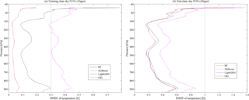
It can be seen from Fig. 11 that the three basic models achieve good retrieval results. In the training sample set, the RMSE of different atmospheric pressure layer temperatures obtained from Random Forest, XGBoost, LightGBM, and generalized ensemble learning are less than 0.786, 0.484, 0.194, and 0.186 K, respectively. Because the retrieval effect of LightGBM is close to that of generalized ensemble learning, the two RMSE curves are nearly coincident. In the testing dataset, although the temperature RMSE of the four models between 1 hPa and 3 hPa is larger, the temperature RMSE of the four models for the majority of pressure layers, between 5 hPa and 1000 hPa, is less than 1 K. Compared with the LightGBM retrieval results in the training and testing dataset, the maximum accuracy of generalized ensemble learning retrieval for temperature profiles is improved by 4.580 % and 5.781 %, respectively.

b. All-sky FOV temperature profile retrieval

High-impact weather is often accompanied by the occurrence and development of clouds (McNally 2002), so it is important to be able to carry out temperature profile retrievals under cloudy FOVs. The nonlinear relationship between brightness temperature and atmospheric variables can be well described based on methods such as Random Forest, without the complex relationship of physical models (Cai et al. 2020). Unlike the retrieval of temperature profiles for clear-sky FOVs, the all-sky FOV samples used for training and testing here include clear-sky and cloudy FOVs.

Figure 12 shows an analysis of the accuracy of temperature profiles retrieved by different models under all-sky FOVs.

Fig. 12

Comparison of the retrieval temperature accuracy of different models under all-sky FOVs: (a) training dataset (four models); (b) testing dataset (four models); (c) training dataset (two models); (d) testing dataset (two models). The temperatures at low altitudes (> 200 hPa) are the most important for meteorological models.

It can be seen from Fig. 12 that the three basic models achieve good results. The RMSE of temperature profiles retrieved from Random Forest, XGBoost, LightGBM, and generalized ensemble learning in the training sample set is less than 0.723, 0.598, 0.323, and 0.284 K, respectively. In the testing dataset, the retrieval accuracy of generalized ensemble learning is better than that of the three basic models. Surprisingly, under the condition of all-sky FOVs (including cloudy FOVs), except for the 1, 2, and 3 hPa pressure layers, the temperature RMSE of all the pressure layers is less than 1 K.

The accuracy and stability of the retrieval algorithm are highly dependent on the representativeness of the training dataset (Zhu et al. 2023). It is found that, at lower levels (below approximately 800 hPa), the retrieval results for the all-sky FOVs have more accurate temperatures than those for the clear-sky FOVs. This may be attributable to the different sample sizes and the high vertical resolution information of the hyperspectral data.

Further research shows that, under the condition of all-sky FOVs, the RMSE of temperature profiles retrieved by the different models is larger at 100–200 hPa than at other pressure layers. This is consistent with the findings of Xue et al. (2022). However, according to Malmgren-Hansen et al. (2019), temperatures at low altitudes (> 200 hPa) are the most important for meteorological models.

It can be seen from Figs. 6, 11, and 12 that the RMSE of all layers of the profile of the generalized ensemble learning temperature in the training dataset is within 0.3 K, while that in the testing dataset is within 1.4 K, and between 150 hPa and 925 hPa it is within 1 K.

Furthermore, Fig. 13 shows the retrieved temperature profile and temperature deviation obtained by using generalized ensemble learning under all-sky FOVs. The deviation here is defined as the difference between the target and retrieval value. The abscissa is the sample number, with a total of 5,120 profiles.

Fig. 13

The (a) target, (b) retrieval temperature profile, and (c) deviation distribution under all-sky FOVs. The abscissa is the sample number, with a total of 5,120 profiles.

Combined with Fig. 13, we can see that, in addition to the upper atmospheric pressure layers, the generalized ensemble learning retrieval of temperature profiles obtains good results.

To analyze the reason for the larger RMSE of 100–200 hPa temperature compared with other pressure layers, the following section discusses the importance of feature variables and the peak layer of the channel weighting function corresponding to important variables. The calculation method of the weighting function is similar to that in Fig. 4.

Figure 14 shows an analysis of the variable importance of the reserved channels (shown in Fig. 3) based on Random Forest after the establishment of the GIIRS channel blacklist. Furthermore, the peak layer distribution of the GIIRS channel weighting function for the top 100 feature variable importance rankings is given. The discussion is divided into clear-sky and all-sky FOVs. Here, the brightness temperature of the GIIRS channel is used as a feature variable for both the basic and ensemble models. The number of channels corresponds to the number of feature variables in the model.

Fig. 14

GIIRS channel importance ranking and weighting function peak layer distribution under (a) clear-sky FOVs (variable importance), (b) all-sky FOVs (variable importance), (c) clear-sky FOVs (peak value of weighting function), and (d) all-sky FOVs (peak value of weighting function).

It can be seen from Fig. 14 that there are no channels selected among the top 100 channels of variable importance between the 0 and 200 hPa pressure layers. In future research, GIIRS shortwave channel data will be added to improve the retrieval accuracy of all pressure layer temperatures.

c. Preliminary analysis of the reasonableness of retrieved temperature profiles under all-sky FOVs

Figure 15 shows the GIIRS channel weighting function distribution of the top 36 Random Forest importance values of the midlatitude summer profile. Note that this is only to explain the reason for the reasonableness of retrieved temperature profiles under all-sky FOVs. The channel brightness temperature distribution of the GIIRS Jacobian (Coopmann et al. 2022) at 0000 UTC 10 August 2019 in different peak layers is further given.

Fig. 15

GIIRS channel weighting function and vertical layer (representative layer) distribution of GIIRS data: (a) weighting function and (b) vertical layer brightness temperature distribution.

The main reason for obtaining better retrieval accuracy under all-sky (clear sky and cloudy) conditions is analyzed. Firstly, we consider the high vertical resolution of GIIRS (Fig. 15a). The peak GIIRS channel weighting function exists in almost every atmospheric pressure layer (Coopmann et al. 2022). The information layers detected by different channels are different, indicating different brightness temperature distributions (Fig. 15b). Some channels may be contaminated by clouds, but other channels may be usable. For example, obtaining the cloud fraction and cloud top pressure (CTP) at a certain FOV through algorithms such as the minimum residual method (Lee et al. 2020), when the peak layer of a certain channel’s weighting function is higher (lower) than the CTP, then the channel is not (is) contaminated by clouds.

Therefore, the channel height assignments cloud detection method of ECMWF (McNally and Watts 2003; Coopmann et al. 2022) utilizes vertical information from hyperspectral data. Secondly, compared to the idealized channel weighting function, the peak layer of the actual weighting function has a certain width (Joiner et al. 2007). This width indicates that the information of the pressure layer near the peak layer can also be detected, so the temperature of the pressure layer nearby can also be retrieved. And thirdly, the training dataset in this paper includes clear-sky and cloud data. The clear-sky data around the clouds plays a certain role in the retrieval of cloud areas (Malmgren-Hansen et al. 2019). In future work, a separate study will be conducted on the retrieval of temperature profiles under cloudy FOVs.

5. Conclusion and future work

Real-time or near-real-time acquisition of vertical temperature profile information is essential for monitoring and forecasting high-impact weather. Geostationary satellite hyperspectral data have the characteristics of high temporal and vertical resolution, which can be used for atmospheric profile retrieval. In this study, based on FY-4A/GIIRS and ERA5 data, the atmospheric temperature profile is retrieved using the generalized ensemble learning and basic models (Random Forest, XGBoost, and LightGBM). The main conclusions can be summarized as follows:

1. (1) Feature variable selection. Based on the establishment of a GIIRS channel blacklist, the feature variables of the basic models are selected by using the permutation importance method. In the Typhoon Lekima experimental case, compared to other channels selected for retrieval models, the importance of mediumwave channels 9 and 307 in GIIRS ranks first and second, respectively.
2. (2) Ensemble weight. On the basis of hyperparameter optimization, generalized ensemble learning is used to optimize the weight of each basic model. The integrated method improves the accuracy of atmospheric temperature profile retrievals. Among the three basic models, XGBoost shows the lowest performance and LightGBM the best. Therefore, compared with the other basic models, LightGBM has the largest ensemble weight value under different pressure layers.
3. (3) Temperature profile retrieval under clear-sky FOVs. The RMSE of the whole temperature profile in the training dataset of the generalized ensemble learning model is less than 0.3 K. The retrieval temperature RMSE of the testing dataset between 150 hPa and 925 hPa is within 1 K. The temperature profiles retrieved by different models correlate well with the target temperature profiles (radiosonde data and ERA5 data).
4. (4) Temperature profile retrieval under all-sky FOVs. The RMSE of temperature profiles retrieved by different models is slightly larger at 0–200 hPa, while that of other pressure layers is less than 1 K. The reason is that no channel is selected among the top 100 channels of variable importance in the 0–200 hPa pressure layer. However, temperatures at low altitudes (> 200 hPa) are the most important for meteorological models (Malmgren-Hansen et al. 2019).

Although the method in this paper achieves good retrieval results, there are also some shortcomings. For example, although high-frequency observation data are used, the sample size of the data of the machine learning algorithm is still small (Ma et al. 2021). Some model parameters (such as max_features and min_samples_split of Random Forest) do not participate in optimization but use default values. In addition, due to the constraints of computing resources, some parameters (such as n_estimators of Random Forest) are set too small. Bias correction of the FY-4A/GIIRS observation data is also not considered, which is important because the existence of bias may affect the establishment of the relationship between the brightness temperature and temperature profile, thereby potentially affecting the accuracy of temperature profile retrievals. Future work should involve building a unified framework while considering the optimization and adjustment of hyperparameters and the weighted integration of basic models. The GIIRS longwave channel or multi-source or multi-dimensional data should be further added to retrieve the atmospheric temperature and humidity profiles. Finally, another step would be to apply the retrieved profile data to the monitoring and forecasting of high-impact weather (Gao et al. 2022).

Data Availability Statement

The GIIRS satellite data and cloud mask product are available at http://satellite.nsmc.org.cn/PortalSite/Data/DataView.aspx?currentculture=en-US (accessed on 11 November 2022). The NCEP reanalysis data can be found at https://rda.ucar.edu/datasets/ds083.2/ (accessed on 11 November 2022). The ERA5 data can be found at https://apps.ecmwf.int/datasets/ (accessed on 11 November 2022).

Acknowledgments

This study was jointly supported by the Key Research and Development Program Projects of Anhui Province (grant no. 2022h11020002), the Anhui Provincial Colleges Science Foundation for Distinguished Young Scholars (grant no. 2022AH020093), the Natural Science Foundation of Anhui Province (2108085QD183), the Anhui Provincial Colleges Excellent Young Talent Support Program Project (grant no. gxyq2022081), the Chaohu University Scientific Research Startup Funding Project (grant no. KYQD-202211), the Chaohu University Discipline Construction Quality Improvement Project (grant no. kj22zsys02), and the National Natural Science Foundation of China (grant no. 41805080). We would like to thank ECMWF, NCEP, and the National Satellite Meteorological Centre for freely providing the ERA5, FNL, and FY-4A/GIIRS data and cloud mask product of FY-4A/AGRI online. We are also very grateful to the reviewers for their careful reviews and highly valuable comments, which led to substantial improvements to this manuscript.

References

•  Aires,  F.,  E.  Boucher, and  V.  Pellet, 2021: Convolutional neural networks for satellite remote sensing at coarse resolution. Application for the SST retrieval using IASI. Remote Sens. Environ., 263, 112553, doi: 10.1016/j.rse.2021.112553.
•  Altmann,  A.,  L.  Toloşi,  O.  Sander, and  T.  Lengauer, 2010: Permutation importance: A corrected feature importance measure. Bioinformatics, 26, 1340–1347.
•  Arai,  K., and  X. M.  Liang, 2009: Sensitivity analysis for air temperature profile estimation methods around the tropopause using simulated Aqua/AIRS data. Adv. Space Res., 43, 845–851.
•  Breiman,  L., 2001: Random forests. Mach. Learn., 45, 5–32.
•  Brown,  G.,  J.  Wyatt,  R.  Harris, and  X.  Yao, 2005: Diversity creation methods: A survey and categorisation. Inform. Fusion., 6, 5–20.
•  Cai,  X.,  Y.  Bao,  G. P.  Petropoulos,  F.  Lu,  Q.  Lu,  L.  Zhu, and  Y.  Wu, 2020: Temperature and humidity profile retrieval from FY4-GIIRS hyperspectral data using artificial neural networks. Remote Sens., 12, 1872, doi: 10.3390/rs12111872.
•  Coopmann,  O.,  N.  Fourrié, and  V.  Guidard, 2022: Analysis of MTG-IRS observations and general channel selection for numerical weather prediction models. Quart. J. Roy. Meteor. Soc., 148, 1864–1885.
•  Di,  D.,  J.  Li,  W.  Han,  W.  Bai,  C.  Wu, and  W. P.  Menzel, 2018: Enhancing the fast radiative transfer model for FengYun-4 GIIRS by using local training profiles. J. Geophys. Res.: Atmos., 123, 12583–12596.
•  Dietterich,  T. G., 2000: Ensemble methods in machine learning. International Workshop on Multiple Classifier Systems. Springer, 1–15.
•  Feng,  Y.,  S.  Fan,  K.  Xia, and  L.  Wang, 2022: Estimation of regional ground-level PM_2.5 concentrations directly from satellite top-of-atmosphere reflectance using a hybrid learning model. Remote Sens., 14, 2714, doi: 10.3390/rs14112714.
•  Gao,  Y.,  D.  Mao,  X.  Wang, and  D.  Qin, 2022: Evaluation of FY-4A temperature profile products and application to winter precipitation type diagnosis in southern China. Remote Sens., 14, 2363, doi: 10.3390/rs14102363.
•  Huang,  P.,  Q.  Guo,  C.  Han,  C.  Zhang,  T.  Yang, and  S.  Huang, 2021: An improved method combining ANN and 1D-Var for the retrieval of atmospheric temperature profiles from FY-4A/GIIRS hyperspectral data. Remote Sens., 13, 481, doi: 10.3390/rs13030481.
•  Jang,  H.-S.,  B.-J.  Sohn,  H.-W.  Chun,  J.  Li, and  E.  Weisz, 2017: Improved AIRS temperature and moisture soundings with local a priori information for the 1DVAR method. J. Atmos. Oceanic Technol., 34, 1083–1095.
•  Joiner,  J.,  E.  Brin,  R.  Treadon,  J.  Derber,  P.  Van Delst,  A.  Da Silva,  J.  Le Marshall,  P.  Poli,  R.  Atlas,  D.  Bungato, and  C.  Cruz, 2007: Effects of data selection and error specification on the assimilation of AIRS data. Quart. J. Roy. Meteor. Soc., 133, 181–196.
•  Ke,  G.,  Q.  Meng,  T.  Finley,  T.  Wang,  W.  Chen,  W.  Ma,  Q.  Ye, and  T.-Y.  Liu, 2017: LightGBM: A highly efficient gradient boosting decision tree. Advances in Neural Information Processing Systems 30.  von Luxburg,  U.,  I.  Guyon,  S.  Bengio,  W.  Hanna,  R.  Fergus (eds.), Curran Associates Inc., 3146–3154.
•  Krogh,  A., and  J.  Vedelsby, 1994: Neural network ensembles, cross validation, and active learning. Advances in Neural Information Processing Systems 7.  Tesauro,  G.,  D. S.  Tourestzky, and  T. K.  Leen (eds.), MIT Press, 231–238.
•  Lee,  A.,  B.-J.  Sohn,  E.  Pavelin,  Y.  Kim,  H.-S.  Kang,  R.  Saunders, and  Y.-C.  Noh, 2020: Assessment of cloud retrieval for IASI 1D-Var cloudy-sky assimilation and improvement with an ANN approach. Wea. Forecasting, 35, 1363–1380.
•  Lee,  S. J.,  M.-H.  Ahn, and  S.-R.  Chung, 2017: Atmospheric profile retrieval algorithm for next generation geostationary satellite of Korea and its application to the advanced Himawari Imager. Remote Sens., 9, 1294, doi: 10.3390/rs9121294.
•  Lee,  Y.,  D.  Han,  M.-H.  Ahn,  J.  Im, and  S. J.  Lee, 2019: Retrieval of total precipitable water from Himawari-8 AHI data: A comparison of random forest, extreme gradient boosting, and deep neural network. Remote Sens., 11, 1741, doi: 10.3390/rs11151741.
•  Li,  J., and  W.  Han, 2017: A step forward toward effectively using hyperspectral IR sounding information in NWP. Adv. Atmos. Sci., 34, 1263–1264.
•  Li,  X.,  J.  Luo,  X.  Jin,  Q.  He, and  Y.  Niu, 2020: Improving soil thickness estimations based on multiple environmental variables with stacking ensemble methods. Remote Sens., 12, 3609, doi: 10.3390/rs12213609.
•  Liu,  Z.,  M.  Min,  J.  Li,  F.  Sun,  D.  Di,  Y.  Ai,  Z.  Li,  D.  Qin,  G.  Li,  Y.  Lin, and  X.  Zhang, 2019: Local severe storm tracking and warning in pre-convection stage from the new generation geostationary weather satellite measurements. Remote Sens., 11, 383, doi: 10.3390/rs11040383.
•  Ma,  Z.,  J.  Li,  W.  Han,  Z.  Li,  Q.  Zeng,  W. P.  Menzel,  T. J.  Schmit,  D.  Di, and  C.-Y.  Liu, 2021: Four-dimensional wind fields from geostationary hyperspectral infrared sounder radiance measurements with high temporal resolution. Geophys. Res. Lett., 48, e2021GL093794, doi: 10.1029/2021GL093794.
•  Maier,  J., and  R.  Knuteson, 2022: Data fusion of GEO FY-4A GIIRS and LEO hyperspectral infrared sounders with surface observations: A Hong Kong case study. J. Atmos. Oceanic Technol., 39, 259–270.
•  Malmgren-Hansen,  D.,  V.  Laparra,  A. A.  Nielsen, and  G.  Camps-Valls, 2019: Statistical retrieval of atmospheric profiles with deep convolutional neural networks. ISPRS J. Photogramm. Remote Sens., 158, 231–240.
•  Marques,  J. P. P. G.,  D. C.  Cunha,  L. M. F.  Harada,  L. N.  Silva, and  I. D.  Silva, 2021: A cost-effective trilateration-based radio localization algorithm using machine learning and sequential least-square programming optimization. Comput. Commun., 177, 1–9.
•  McNally,  A. P., 2002: A note on the occurrence of cloud in meteorologically sensitive areas and the implications for advanced infrared sounders. Quart. J. Roy. Meteor. Soc., 128, 2551–2556.
•  McNally,  A. P., and  P. D.  Watts, 2003: A cloud detection algorithm for high-spectral-resolution infrared sounders. Quart. J. Roy. Meteor. Soc., 129, 3411–3423.
•  Menzel,  W. P.,  T. J.  Schmit,  P.  Zhang, and  J.  Li, 2018: Satellite-based atmospheric infrared sounder development and applications. Bull. Amer. Meteor. Soc., 99, 583–603.
•  Min,  M.,  C.  Wu,  C.  Li,  H.  Liu,  N.  Xu,  X.  Wu,  L.  Chen,  F.  Wang,  F.  Sun,  D.  Qin,  X.  Wang,  B.  Li,  Z.  Zheng,  G.  Cao, and  L.  Dong, 2017: Developing the science product algorithm testbed for Chinese next-generation geostationary meteorological satellites: Fengyun-4 series. J. Meteor. Res., 31, 708–719.
•  Noh,  Y.-C.,  B.-J.  Sohn,  Y.  Kim,  S.  Joo,  W.  Bell, and  R.  Saunders, 2017: A new infrared atmospheric sounding interferometer channel selection and assessment of its impact on Met Office NWP forecasts. Adv. Atmos. Sci., 34, 1265–1281.
•  Saunders,  R.,  J.  Hocking,  E.  Turner,  P.  Rayer,  D.  Rundle,  P.  Brunel,  J.  Vidot,  P.  Roquet,  M.  Matricardi,  A.  Geer,  N.  Bormann, and  C.  Lupu, 2018: An update on the RTTOV fast radiative transfer model (currently at version 12). Geosci. Model Dev., 11, 2717–2737.
•  Shahhosseini,  M.,  G.  Hu, and  H.  Pham, 2022: Optimizing ensemble weights and hyperparameters of machine learning models for regression problems. Mach. Learn. Appl., 7, 100251, doi: 10.1016/j.mlwa.2022.100251.
•  Smith,  W. L.,  E.  Weisz,  S. V.  Kireev,  D. K.  Zhou,  Z.  Li, and  E. E.  Borbas, 2012: Dual-regression retrieval algorithm for real-time processing of satellite ultraspectral radiances. J. Appl. Meteor. Climatol., 51, 1455–1476.
•  Strobl,  C.,  A. L.  Boulesteix,  A.  Zeileis, and  T.  Hothorn, 2007: Bias in random forest variable importance measures: Illustrations, sources and a solution. BMC Bioinformatics, 8, 1–21.
•  Wang,  G.,  W.  Han, and  S.  Lu, 2021: Precipitation retrieval by the L1-norm regularization: Typhoon Hagibis case. Quart. J. Roy. Meteor. Soc., 147, 773–785.
•  Xue,  Q.,  L.  Guan, and  X.  Shi, 2022: One-dimensional variational retrieval of temperature and humidity profiles from the FY4A GIIRS. Adv. Atmos. Sci., 39, 471–486.
•  Yang,  J.,  Z.  Zhang,  C.  Wei,  F.  Lu, and  Q.  Guo, 2017: Introducing the new generation of Chinese geostationary weather satellites, Fengyun-4 (FY-4). Bull. Amer. Meteor. Soc., 98, 1637–1658.
•  Yin,  R.,  W.  Han,  Z.  Gao, and  D.  Di, 2020: The evaluation of FY4A’s Geostationary Interferometric Infrared Sounder (GIIRS) long-wave temperature sounding channels using the GRAPES global 4D-Var. Quart. J. Roy. Meteor. Soc., 146, 1459–1476.
•  Zhang,  J.,  Z.  Li,  J.  Li, and  J.  Li, 2014: Ensemble retrieval of atmospheric temperature profiles from AIRS. Adv. Atmos. Sci., 31, 559–569.
•  Zhang,  K.,  C.  Wu, and  J.  Li, 2016: Retrieval of atmospheric temperature and moisture vertical profiles from satellite Advanced Infrared Sounder radiances with a new regularization parameter selecting method. J. Meteor. Res., 30, 356–370.
•  Zhang,  Q.,  Y.  Yu,  W.  Zhang,  T.  Luo, and  X.  Wang, 2019: Cloud detection from FY-4A’s geostationary interferometric infrared sounder using machine learning approaches. Remote Sens., 11, 3035, doi: 10.3390/rs11243035.
•  Zhou,  D. K.,  W. L.  Smith,  X.  Liu,  A. M.  Larar,  S. A.  Mango, and  H.-L.  Huang, 2007: Physically retrieving cloud and thermodynamic parameters from ultraspectral IR measurements. J. Atmos. Sci., 64, 969–982.
•  Zhu,  L.,  Y.  Bao,  G.  Petropoulos,  P.  Zhang,  F.  Lu,  Q.  Lu,  Y.  Wu, and  D.  Xu, 2020: Temperature and humidity profiles retrieval in a plain area from Fengyun-3D/HIRAS sensor using a 1D-VAR assimilation scheme. Remote Sens., 12, 435, doi: 10.3390/rs12030435.
•  Zhu,  L.,  R.  Zhou,  D.  Di,  W.  Bai, and  Z.  Liu, 2023: Retrieval of atmospheric water vapor content in the environment from AHI/H8 using both physical and random forest methods—A case study for Typhoon Maria (201808). Remote Sens., 15, 498, doi: 10.3390/rs15020498.