Article
Dispersion Simulation Using the 1-km Gridded Wind Fields Constructed by Super-Resolution Surrogate Downscaling
2025 年 103 巻 3 号 p. 321-333

詳細
2025 年 103 巻 3 号 p. 321-333
Surrogate downscaling is one of the most promising applications of deep learning techniques in meteorology. Sekiyama et al. (2023), a companion paper to this study, employed a super-resolution surrogate downscaling (SRSD) scheme to construct 1-km gridded wind fields from 5-km gridded operational weather forecasts. The SRSD model functions at a much lower computational load than physics-based weather forecast models do to downscale wind fields. This study presents a dispersion simulation, in which fluid dynamics are physics-based but driven by the SRSD’s wind fields, reproducing air pollution plumes over complex terrain near Tokyo. The purpose of this study is to demonstrate the accuracy of not only the SRSD’s wind fields but also the dispersion simulation driven by the SRSD’s wind fields. The SRSD’s wind-driven dispersion model (1-km grid) yielded better statistical scores than a lower-resolution physics-based model (5-km grid). In the snapshots of air pollution plumes, the SRSD’s wind-driven dispersion reproduced reasonable distributions in physics, such as horizontally diverted and blocked plumes around steep terrain and highland areas, better than the lower-resolution physics-based model did. Although a perfect surrogate of higher-resolution physics-based dispersion models cannot be achieved, our strategy can support air pollution dispersion simulations considering the overwhelming difference in the wind downscaling forecast speed between the SRSD and physics-based schemes. This strategy must be beneficial for environmental emergency responses.
Low-resolution atmospheric models never duplicate the grid averages of high-resolution atmospheric models. This is because numerical models demonstrate a resolution dependence of physical and topographical parameterizations. In particular, wind fields in the planetary boundary layer (PBL) are strongly affected by the complexity of model topography (Sekiyama and Kajino 2020; Suzuki et al. 2021). Moreover, low-resolution models often have a front position bias near coastal areas, which is strongly dependent on model resolution (Sekiyama and Kajino 2020; Suzuki et al. 2021). Therefore, low-resolution models cannot be substituted for high-resolution models in the PBL even if low-resolution models have good performance for large-scale dispersion simulations (Sekiyama et al. 2015; Sekiyama and Kajino 2021). Moreover, high-resolution models consume large amounts of computational resources as long as we use conventional methods (i.e., physics-based numerical simulations) for downscaling (i.e., a procedure to infer high-resolution variables from low-resolution variables). This deficiency in model simulation becomes critical in environmental emergency responses (EER; cf. World Meteorological Organization 2006) over complex terrain. The EER situation requires a quick response, while computational resources for dispersion simulations are often limited.
Recent advancements in artificial intelligence (AI) technology have led to the development of surrogate downscaling methods (e.g., temperature/precipitation fields by Baño-Medina et al. 2020; wind fields by Höhlein et al. 2020 or Sekiyama et al. 2023). These studies employ a super-resolution (SR) technique (Yang et al. 2019; Wang et al. 2020), where high-resolution photographic images are generated from low-resolution images via deep neural networks. The advantage of super-resolution surrogate downscaling (SRSD) is its computational speed. For example, Sekiyama et al. (2023) reported that their SRSD model could run three orders of magnitude faster than a physics-based downscaling model when downscaling a single-layer wind field, even if the SRSD model was operated with only one GPU and the physics-based model was operated with more than one hundred CPUs.
Sekiyama et al. (2023) investigated the accuracy of the PBL wind fields constructed by their SRSD model, which downscaled 5-km gridded operational forecasts to 1-km gridded forecasts. They aimed at high-resolution air pollution dispersion simulations over complex terrain at low computational costs, where the SRSD model provided the time series of wind fields. They intended to perform dispersion simulations via a physics-based model. However, while they confirmed the good performance of the SRSD model, they did not perform dispersion simulations using the SRSD wind fields. The purpose of this study is to conduct the dispersion simulations left undone by Sekiyama et al. (2023). In this study, the 1-km dispersion simulations driven by the SRSD wind fields are compared with physics-based 1-km and 5-km dispersion simulations.
Generally, model advection errors consist of wind velocity errors accumulated along advection routes (Sekiyama et al. 2017, 2021). Consequently, as Sekiyama and Kajino (2020) reported, pollution plume distributions sometimes do not match at all over complex terrain between low-resolution and high-resolution dispersion models even if the model errors in the wind fields are relatively small. Thus, the dispersion model performance in this study will be worse than the SRSD model performance in Sekiyama et al. (2023). However, even if perfect surrogate downscaling is not achieved, the concept of this study is that the SRSD wind fields could be used as an alternative to expensive physics-based wind fields, considering the overwhelming difference in the downscaling speed. Notably, the SRSD wind fields are merely the boundary conditions in this study. The dispersion models are not surrogated directly. Typically, for dispersion simulations, low-resolution wind fields can be easily obtained from governmental operational weather forecasts, for example, which are gridded 5-km datasets in Japan as of 2024. Moreover, the most expensive process for high-resolution dispersion simulations is to obtain high-resolution wind fields. Therefore, once we obtain high-resolution wind fields, the difficulty of high-resolution dispersion simulations is greatly reduced. This paper shows the possibility of such economical dispersion simulations, which must be beneficial for EER systems.
When Sekiyama et al. (2023) constructed 1-km gridded SRSD wind fields, they prepared meteorological variables as training, validation, and test data via 5-km and 1-km gridded weather forecast models. The datasets are available from Sekiyama (2023). The weather forecast models, which are based on a governmental operational model (Saito et al. 2006, 2007; Japan Meteorological Agency 2022), are physics-based, mesoscale-oriented, and nonhydrostatic and comprise 59 vertical layers from the surface to approximately 21 km. The 1-km gridded weather forecast model is nested with the 5-km model. Both models are identical except for the horizontal area and resolution, time intervals, and cumulus parameterizations. The meteorological dataset was prepared for 10 years from 2010 to 2019 via the boundary conditions derived from 3-hourly operational mesoscale analyses (Japan Meteorological Agency 2022). The period from 2010 to 2017 was used for SRSD training. The data from 2018 were used for prediction examination, whereas the data from 2019 were used for validation.
Sekiyama et al. (2023) constructed SRSD wind fields by employing a convolutional deep neural network (CDNN), which combines a U-Net architecture (Ronneberger et al. 2015) and a ResNet architecture (He et al. 2016). The loss function contains four terms: the cosine dissimilarity (CosDis), the magnitude difference (MagDif), the divergence difference, and the curl difference for horizontal wind fields. Given the target wind vector ti and the predicted wind vector yi at location i, the CosDis and MagDif are defined as follows:
 |
and
 |
where ·, || ||, and | | indicate the inner product, vector length, and absolute value, respectively. When the two vectors are identical, the CosDis is zero. When the angles between the two vectors are 11.25° (1 in 32 directions), 22.5° (1 in 16 directions), and 45° (1 in 8 directions), the CosDis are 0.01, 0.04, and 0.15, respectively. An angle of 90° (180°) results in a CosDis of 0.5 (1.0).
The predictands were 1-km gridded zonal (east-west) and meridional (south-north) winds. The predictors were the 1-km gridded land/water surface elevation and land/water ratio as well as the 5-km gridded zonal and meridional winds, temperature, humidity, vertical gradient of potential temperature, land/water surface elevation, and land/water ratio. Sekiyama et al. (2023) employed 20-member ensemble predictions to stably obtain a single-layer wind field. The details of the weather forecast simulation and the SRSD process are described in Sekiyama et al. (2023). We use the same CDNN model and SRSD process as those of Sekiyama et al. (2023) to obtain the SRSD wind fields.
As in Sekiyama et al. (2023), the SRSD target domain was cropped to a 180 km × 180 km (Fig. 1a) from the physics-based model domain. The SRSD target domain contains mountainous, plain, and bay areas, such as Mount Fuji, the Tokyo city area, and Tokyo Bay. The sizes of the 5-km and 1-km gridded fields were 36 × 36 and 180 × 180 pixels, as shown in Figs. 1b and 1c. Although Sekiyama et al. (2023) computed only a single-layer surface wind field, we need multiple layers in the PBL to perform local dispersion simulations. Therefore, we separately trained six SRSD models for six layers using each layer’s meteorological variables as training data. The elevations of the six layers were 20 m (defined as the surface layer), 111, 248, 431, 659, and 932 m above ground. These elevations correspond to the first, third, fifth, seventh, ninth, and eleventh layers of our weather forecast model. Typically, the vertical resolution of weather forecast datasets available from official weather services is comparable to these elevations. The 1-km gridded SRSD wind fields were independently calculated at each layer via each SRSD model. All the meteorological data, both physics-based and SRSD-based, were prepared and stored hourly from January 1 to December 31, 2018, to input into the dispersion model.

(a) Model domain of the 5-km gridded physics-based weather forecast model used for meteorological variable preparation. The target domain of the SRSD with the topography of the (b) 5-km gridded and (c) 1-km gridded weather forecast models. The blue areas indicate water surfaces.
Air pollution dispersion was calculated via an offline Eulerian regional air quality model, which was driven by the meteorological variables described in the previous section. This offline dispersion model was developed and evaluated by Kajino et al. (2012, 2018, 2019a, b), Mathieu et al. (2018), Sekiyama and Kajino (2020, 2021), and Sekiyama et al. (2015, 2017, 2021). In this study, virtual pollutants are constantly (1 Tmol h−1) emitted from a single-grid surface source in Shinjuku, Tokyo, where Tokyo Metropolitan City Hall stands in the real world (35.69°N, 139.69°E; shown in Figs. 1b, c as the black filled circle “Tokyo”). This location is suitable for dispersion simulation tests over complex terrain because it is on the edge of the Kanto Plain, close to coastal and mountainous areas. The pollutants are assumed to be completely inert, volatile, and not affected by wet/dry depositions. The pollutants disappear outside the model domain. Therefore, the returning pollutants cannot be considered.
The offline dispersion model shares the same horizontal and vertical domains as the SRSD wind fields (i.e., Figs. 1b, c). The model top height is identical to that of the sixth layer of the SRSD wind fields. The meteorological variables are input at 1-h intervals and linearly time-interpolated. This time-interpolation from 1-h intervals to dispersion time intervals (e.g., 3 sec for this study) has been commonly used in previous studies (Kajino et al. 2012, 2018, 2019a, b; Mathieu et al. 2018; Sekiyama et al. 2015, 2017, 2021; Iwasaki et al. 2019; Sekiyama and Kajino 2020, 2021). In these previous studies, the time-interpolation worked well, with horizontal resolutions ranging from 250 m to more than 10 km and vertical resolutions not significantly different from this study. The vertical resolution of the dispersion model is twice as high as that of the SRSD wind fields so that the input variables are linearly interpolated between adjacent SRSD layers. The dispersion simulations are continuously performed for one year from January 1 to December 31, 2018. The dispersion model outputs are stored at 1-h intervals to calculate statistical scores.
The offline dispersion model requires inputs of not only horizontal winds but also other meteorological variables, such as vertical wind, temperature, pressure, and eddy diffusivity. These variables are obtained from the meteorological datasets generated by the physics-based weather forecast models along with the training, validation, and test data. However, only vertical winds are diagnostically calculated from horizontal wind divergence/convergence via a mass-conservative scheme (Ishikawa et al. 1994). Note that this study does not downscale meteorological variables other than horizontal winds; i.e., we do not have 1-km gridded variables other than horizontal winds when performing dispersion simulations. Therefore, all the experiments other than the reference experiment utilize 5-km gridded meteorological variables except for 1-km gridded horizontal winds.
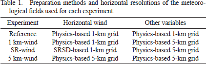
We perform four experiments in this study, as shown in Table 1. The reference simulation is driven by both the 1-km gridded horizontal winds and other meteorological variables calculated by the 1-km gridded physics-based weather forecast model. In the 1-km gridded wind experiment (hereafter named “1 km-wind”), horizontal winds are derived from the 1-km gridded physics-based model, but the others are derived from the 5-km gridded physics-based model. In the 5-km gridded wind experiment (hereafter named “5 km-wind”), all the variables are derived from the 5-km gridded physics-based model. The 1-km gridded SRSD horizontal winds are used only for the “SR-wind” experiment, in which the other variables are derived from the 5-km gridded physics-based model. Note that all the 5-km gridded variables are bilinearly interpolated to the 1-km model resolution. Therefore, the four experiments, including the 5-km wind experiment, are performed with a 1-km dynamical resolution.
First, we assume that the reference simulation provides the truth of the concentration distributions. We investigate the performance of the dispersion simulations (1 km-wind, SR-wind, and 5 km-wind) via several metrics. The metrics measure the degree of agreement in the air pollution plume distribution. One of the metrics is Pearson’s correlation (hereafter, just called “correlation”). Another is structural similarity (SSIM) (Wang et al. 2004; Doan et al. 2021), which is defined as follows:
 |
where μx, μy,  , and σxy. are the mean length of vector x, the mean length of vector y, the variance of vector x, the variance of vector y, and the covariance of vectors x and y, respectively. The original formula of the SSIM is more intricate for measuring the quality of television or movie pictures (Wang et al. 2004), which compares the brightness, contrast, and structural differences between two image vectors. However, Doan et al. (2021) indicated that the original formula can be simplified to Eq. (3) and successfully used as a loss function to classify synoptic weather charts via machine learning. In this study, we use Eq. (3) to measure the similarity of the strength and structure between two distributions by averaging over the target area. The SSIM ranges from −1 to 1, where 1 indicates that the two distributions are identical. When SSIM = 0, the two distributions are completely independent.
Furthermore, we measure the similarity via statistical recall and specificity with a threshold concentration. Before these statistical scores are defined, the following numbers should be used:
True Positive (TP): the number of truly positive predictions that correctly exceed the threshold concentration when the truth exceeds it as well (i.e., correct hits); True Negative (TN): the number of truly negative predictions that correctly fall short of the threshold concentration when the truth falls short as well (i.e., correct rejections);
False Positive (FP): the number of false-positive predictions that incorrectly exceed the threshold concentration, although the truth falls short (i.e., false alarms); False Negative (FN): the number of false-negative predictions that incorrectly fall short of the threshold concentration although the truth exceeds it (i.e., misses).
Recall is defined as the ratio of the number of TPs to the number of positive reference events (TP + FN):
 |
Generally, a lower recall score is inadequate for disaster prevention because it misses many positive events. However, when the TP is much smaller than others (i.e., rare events, such as tornado outbreaks, typhoon damage, and very narrow plume contamination), the recall score tends to be lower or unstable. Specificity is defined as the ratio of the number of TNs to the number of negative reference events (TN + FP):
 |
A higher specificity score often accompanies a lower recall score, and vice versa. For example, if a weather forecaster always foretells a negative result, the specificity will be 1, but the recall will be 0. Therefore, if either of the scores is unnaturally good, the statistics are not very reliable and need attention.
Here, the crucial point is how the threshold concentration should be determined for correctly evaluating the recall and specificity. The threshold regulates the range of a plume distribution. Single-point source dispersion simulations, such as those in this study, typically produce a clearly edged pollution plume, with borders where concentration values jump by thousands or millions of times (Iwasaki et al. 2019). Therefore, small changes in the threshold concentration do not have a large effect on the statistical scores used to compare two plume structures or locations. We only need to adjust the number of digits for the threshold, as shown in Table 2. This table shows the percentages of TPs, FPs, and FNs for the SR-wind experiment throughout 2018 over the entire domain at the ground surface. When the threshold is low, plumes become broader, and then the TPs increase, which makes the recall unnaturally good. However, if the threshold is too high, not only the TPs but also the FPs and the FNs become very small (i.e., the TNs is extremely large), which makes the specificity unnaturally good. A good threshold should ensure that TPs is not too large but FPs and FNs are not too small. Therefore, we set the threshold concentration as 10−1 mol m−3 on the basis of the results in Table 2. In addition, the 10 % of the domain width (18 pixels) around the borders was not used in the metric calculations to avoid the adverse effects of the lateral boundaries.

Before investigating the performance of the dispersion simulations, we examine the accuracy of the SRSD wind fields constructed for this study. Figure 2 shows the monthly averaged CosDis and MagDif between the 1-km gridded target and the SRSD input/output at model layers 1 (L-1; 20 m), 3 (L-3; 248 m), and 6 (L-6; 932 m) over the whole domain. At model layer 1 (i.e., ground surface; black lines in Fig. 2a), the CosDis scores, i.e., the direction errors, are improved from 0.10–0.13 (approximately “1 off in 8 directions”) to 0.04–0.07 (approximately “1 off in 16 directions”) by the SRSD model. This is consistent with the results of Sekiyama et al. (2023). The higher the elevation is, the smaller the 5-km gridded input direction errors (blue and red circles in Fig. 2a). This is because the influence of complex terrains decreases at higher layers. Nevertheless, the output direction errors (blue and red stars in Fig. 2a) are consistently smaller than the input direction errors at higher layers.

Monthly averaged (a) CosDis and (b) Mag Dif between the 1-km gridded target (i.e., truth) and the SRSD input/output over the model domain at model layers 1 (20 m), 3 (248 m), and 6 (932 m).
In contrast, the MagDif scores, i.e., the wind speed errors, are greater in the higher layers (L-3 and L-6) than in the lower layer (L-1), as shown in Fig. 2b. This is simply because higher altitude winds are faster than surface winds. At both L-3 and L-6, the input speed errors (blue and red circles; approximately 1.0–1.5 m s−1) are improved by half or 2/3 compared to the output speed errors of approximately 0.6–0.9 m s−1 (blue and red stars). Although the absolute values are smaller than those at L-3 and L-6, the improvement ratios of the wind speeds at L-1 (ground surface) are almost the same, approximately half or 2/3, as shown in Fig. 2b (black circles and stars), where the surface wind speed errors are improved from 0.7–0.8 m s−1 to 0.4–0.5 m s−1. Overall, the SRSD models worked well, as presented by Sekiyama et al. (2023), not only for surface winds but also for upper-level winds in the PBL.
The results of the other layers (L-2, L-4, and L-5) for both the CosDis and MagDif scores are not shown in Fig. 2 but settle in the ranges easily inferred from the results of L-1, L-3, and L-6. In general, the performance degradation in the CosDis scores tends to occur when the wind velocity is large and simultaneously it changes abruptly (Sekiyama 2023), as discussed later. On the other hand, the degradation in the MagDif scores occurs just when the wind velocity is large because if the error rate is constant, the absolute error becomes large when the wind is strong. In Japan, the wind speed tends to be higher in winter than in summer because of the monsoon except for the influence of typhoons. These are probably the sources of the seasonal variation in the scores.
3.2 Dispersion simulation performanceFigure 3 shows the monthly average correlation/SSIM/recall/specificity over the dispersion model domain at the ground surface for each experiment, assuming that the reference is the true plume concentration. In general, the 1 km-wind simulation displays very high scores for all four indices (black and red stars in Fig. 3), although it does not perfectly match the reference. The SR-wind simulation (black and red circles) is always superior to the 5 km-wind simulation (black and red triangles) for all four indices. However, the difference between the 1 km-wind and the SR-wind scores is greater than that between the SR-wind and 5 km-wind scores. In other words, the SR-wind dispersion is closer to the 5 km-wind dispersion rather than the 1 km-wind dispersion. Note that the specificity scores are always high throughout the year for all the experiments (black stars, circles, and triangles in Fig. 3b). The reason for this feature is described and discussed later.

Monthly averaged (a) Pearson’s correlation, structural similarity (SSIM), (b) specificity, and recall over the dispersion model domain at the ground surface for each experiment. The target is the reference experiment result with a threshold of 10−1 mol m−3.
Figure 4 shows the hourly time series of correlation/SSIM/recall/specificity over the dispersion model domain at the ground surface for each experiment. These values are not temporally averaged. This period (October 15–18, 2018) was selected because the plumes drastically changed in direction during a short period, as illustrated later. Unlike the monthly averages, Fig. 4 shows large fluctuations in each index. The 1 km-wind simulation (black and red stars in Figs. 4a, b) displays the smallest fluctuations among the three experiments, keeping the scores close to 1 except for the SSIM scores. The excellent performance of the 1 km-wind model indicates that dispersion models function well even when high-resolution meteorological variables other than horizontal winds cannot be obtained. In general, the SSIM score deteriorates sensitively even with very small strength/structure/location errors.

Hourly time series of (a) Pearson’s correlation, structural similarity (SSIM), (b) specificity, recall, and (c) the areas of FN/TP/FP over the dispersion model domain at the ground surface for 4 days from 00 UTC October 15 to 00 UTC October 19, 2018. The threshold for specificity, recall, and plume area definition is 10−1 mol m−3.
Compared with the 1 km-wind simulation, the SR-wind and 5 km-wind simulations are not stable. The SSIM, correlation, and recall for the 5 km-wind simulation (black lines in Fig. 4) often decrease to less than 0.5, whereas those for the SR-wind simulation (red lines in Fig. 4) maintain higher performance in many cases. The specificity deteriorates on October 15 and 16 (the first two days) but is almost perfect on October 17 and 18 (the latter two days) for all three experiments. In contrast, the recall is relatively good on the first two days but extremely poor on the latter two days. In particular, the recall for the 5 km-wind simulation is 0.1–0.3 for a long time on the latter two days, which means that the 5 km-wind simulation is completely nonfunctional during that time.
We therefore calculated the FN, TP, and FP areas of the simulated plume from the 5 km-wind experiment during this period (Fig. 4c). This classification chart clearly shows the difference between the first two days and the latter two days. The plume is larger in the first half and smaller in the latter half. Figure 5 shows snapshot maps of the horizontal plume distribution at the surface layer during this period. The lightest red plume areas represent the threshold concentration. Consistent with Fig. 4c, the snapshots illustrate that the plume is broadly sweeping at times A and B and narrowly trailing at times C and D. Note that the 1 km-wind result is almost indistinguishable from the “Target” reference to the naked eye even when the metric scores are not exactly 1.

Snapshots of the surface horizontal plume distribution at times A, B, C, and D shown in Fig. 4a. The “Target” illustrates the reference experiment result. The lightest red areas represent the threshold concentration of 0.1 mol m−3. All the topographical contours are drawn on the basis of the elevation and resolution in the 1-km gridded model.
The SR-wind result is more similar to the “Target” reference than to the 5 km-wind result in all snapshots A, B, C, and D. Specifically, in snapshot A, the SR-wind plume moves toward the northwest just after it is emitted from the source, as the reference and 1 km-wind plumes do, although they slightly meander. However, the 5 km-wind plume flows in the opposite direction at this time, which has a completely different tail distribution over the mountainous region from the others. These detailed differences in the plume shapes make the SSIM and correlation significantly worse at time A. In contrast, the recall is not very poor at this time because the areas of the plumes are quite large and then overlap with each other, which makes the area of TPs relatively large, as shown in Fig. 4c.
In contrast, the plumes are very narrow and straight at time C for all the experiments. Consequently, the SSIM, correlation, and specificity scores are very high. In fact, this plume structure appears most frequently throughout the year, which makes the difference between the 1-km and 5-km gridded simulations seem small. However, when the plumes flow into the mountainous area, even if the tails are narrow, the distribution difference becomes pronounced, as shown in snapshot D. At this time, the plumes other than the 5 km-wind plume divert to the north of the peninsula and then surround Mt. Fuji to avoid steep terrain and highland areas. Only the 5 km-wind plume flows straight and does not divert to the north of the peninsula because the 5-km gridded topographies are too gentle to block the plume. Consequently, the 5 km-wind result is extremely degraded at time D, except for the specificity.
While the recall scores are very poor, the specificity scores are close to 1 not only for the 1 km-wind and SR-wind simulations but also for the 5 km-wind simulation at time D. During the latter two days, because the plume areas are very small (Fig. 4c), the FN/TP ratio becomes large (i.e., misses tend to be more frequent than correct hits because a small plume shift easily diminishes plume overlap). As a result, the recall becomes significantly worse. In contrast, under the circumstances of the latter two days, the TN area becomes extremely large because the entire area, with the exception of FNs, TPs, and FPs, within the model domain is the TN area (i.e., the overwhelming majority is “no target and no prediction”). Consequently, the specificity score becomes unnaturally good.
When either the recall or the specificity is unnaturally good, the plumes are too broad or too narrow to adequately perform the model comparison. Therefore, the statistics that exclude these events should also be checked. The monthly averaged recall (specificity) is recalculated to select samples only when the recall (specificity) for the 5 km-wind experiment is less than 0.8 (Fig. 6). Here, the SSIM and correlation coefficient are calculated when either the recall or the specificity is less than 0.8. The recall is calculated with 75 % of the samples, the specificity with 6 % of the samples, and the SSIM/correlation with 77 % of the samples. Even after recalculation, the change in the SSIM and the correlation is not large (see Figs. 3a, 6a). On the other hand, the recall and specificity exhibit a large change after recalculation (see Figs. 3b, 6b). For both metrics, the scores for the 1 km-wind simulation do not substantially change. In contrast, the score gaps between the SR-wind and 5 km-wind simulations increase, as shown in Fig. 6 and listed in Table 3. This finding indicates that the SR-wind model is more robust than the 5 km-wind model under the condition of model performance degradation.

Same as Fig. 3, but the recall (specificity) is averaged only when the recall (specificity) for the 5 km-wind experiment is less than 0.8.

First, the 1 km-wind simulation is an unrealistic setup experiment, where the horizontal winds are obtained from the high-resolution physics-based model nested by a low-resolution model, but the other meteorological variables cannot be obtained from the high-resolution model. It is not surprising that the 1 km-wind simulation shows extremely high agreement with the reference run because both are driven by the same high-resolution wind fields. Instead, the fact that the 1 km-wind simulation maintains high scores throughout the year indicates that high-resolution dispersion models function well if only high-resolution horizontal wind fields are available. The other input variables are not top priorities. Therefore, developing a dispersion model driven by the combination of high-resolution horizontal winds and low-resolution other meteorological variables (other than the wind) is important.
A comparison of the snapshot maps (Fig. 5) reveals that the difference between the SR-wind and 5 km-wind plumes is evident. The SR-wind plume has distributions that reflect real terrain structures (e.g., snapshot A or D), but the 5 km-wind plume does not. Notably, the SRSD model is able to reproduce diverted and blocked wind flows around steep terrain and highland areas. We do need a high-resolution dispersion model when the wind field is affected by complex terrain and low-resolution models cannot reproduce diverted and blocked plumes.
Previous studies on the Fukushima nuclear accident (Nakajima et al. 2017; Sekiyama and Kajino 2020) revealed that air pollution plumes flowing in Fukushima (150 km apart from the Tokyo area) were disturbed by complex terrain for only 10 % or less of the total time during the three weeks after the accident. The wind fields used in this study were also often stable (i.e., not disturbed) throughout the year. When the wind field is not disturbed by complex terrain, the difference between the high-resolution and low-resolution simulations is small, as shown in snapshot C (Fig. 5). Therefore, to clearly distinguish the performance of the SRSD-wind model from that of the 5 km-wind model, it is reasonable to average the statistical scores only when the plumes are disturbed (i.e., recall or specificity less than 0.8 in this study), as shown in Fig. 6.
The SR-wind model is more accurate than the 5 km-wind model is, especially when the statistics deteriorate, i.e., the wind fields are disturbed, as shown by the comparison between Figs. 3b and 6b. In addition, Fig. 6 shows that there is a seasonal variation in the performance of the SR-wind and 5 km-wind models. For the specificity (black lines in Fig. 6b), the SR-wind model scores significantly higher than the 5 km-wind model in the winter and spring seasons. The SR-wind scores are comparable to the 1 km-wind scores in those seasons. In contrast, the difference between the SR-wind and 5 km-wind scores decreases in the summer. Similarly, for the recall (red lines in Fig. 6b), the SR-wind model performs better in the winter, spring, and late fall seasons. However, its performance worsens from July to September. The SSIM and correlation scores for the SR-wind and 5 km-wind models are also extremely poor in August and September.
The main reason for this poor summer performance might be the passage of typhoons over the model domain. According to the Japan Meteorological Agency (JMA), the Tokyo area was approached by typhoons once in June, once in July, twice in August, twice in September (partly in October), and zero times in other months in 2018 (https://www.data.jma.go.jp/fcd/yoho/typhoon/statistics/index.html; in Japanese). Generally, the SRSD performance for wind fields (Sekiyama 2023) deteriorates significantly when the wind is stormily strong and its direction/speed changes abruptly. Therefore, the performance is probably affected more by strong storm systems such as typhoons than by regular extratropical cyclones or winter monsoon winds. It is a future challenge to improve the accuracy of plume dispersion downscaling over complex terrain under the extreme conditions. Nevertheless, the SR-wind model performs better than the 5 km-wind model even in the typhoon season and much better in other seasons. Therefore, given the small computational burden required for SRSD prediction, its use in emergency forecast systems, such as the EER system over complex terrain, is highly promising.
We confirmed that the wind fields constructed by the SRSD model, i.e., a deep learning technique, were able to drive a physics-based dispersion model stably for one year. The dispersion model with the SRSD wind fields was robust and yielded better scores on average than a lower-resolution physics-based model. In the snapshots of air pollution plumes, the dispersion model with the SRSD wind fields reproduced reasonable distributions in physics, such as horizontally diverted and blocked plumes around steep terrain and highland areas, better than a lower-resolution physics-based model. Although a perfect surrogate of high-resolution physics-based models cannot be achieved, our strategy was capable of supporting air pollution dispersion models, given the overwhelming speed of the wind downscaling calculation. Sekiyama et al. (2023) reported that the SRSD model downscaled a single-layer wind field three orders of magnitude faster than a physics-based model even when the SRSD model was operated with only one GPU and the physics-based model was operated with 128 Xeon CPUs.
On the other hand, in the field of technology for global weather forecasts, the development of AI-powered forecast models that do not use physics rapidly progressed after 2023 (e.g., Bi et al. 2023; Lam et al. 2023; Bodnar et al. 2024). These models use AI (i.e., deep neural networks) for water vapor dispersion calculations. Therefore, their architectures are likely to be directly applicable to air pollution dispersion simulations, although successful global calculations do not necessarily guarantee successful mesoscale calculations over complex terrain. Moreover, the AI-powered forecast models require enormous computational resources for training processes. For example, while Sekiyama et al. (2023) spent half a day with a single GPU for the AI training, Bi et al. (2023) spent 16 days with approximately 200 GPUs, and Bodnar et al. (2024) spent two and a half weeks with 32 GPUs. Each GPU is much higher-priced than a high-end CPU. In this respect, our study uses the AI model only for wind field downscaling; therefore, its training process is overwhelmingly inexpensive in comparison with that of AI-powered forecast models. Taking advantage of this economical approach, we should also aim for the social EER implementation of an AI/physics hybrid model, such as the dispersion model with the SRSD wind fields.
The source codes of the SRSD model and its datasets are available from Sekiyama (2023). The source codes of the dispersion model are available under a collaborative framework between the JMA and related institutes/universities. The source codes of the weather forecast model are available subject to a license agreement with the JMA (contact the JMA headquarters at pfm@npd.kishou.go.jp for further information). The JMA operational mesoscale analysis data are provided by the Japanese government via the Japan Meteorological Business Support Center (https://wwwjmbsc.orjp/en/index-e.html), which are freely available for research purposes. All the data used in this paper can also be provided upon request to the corresponding author.
Supplement 1 is a movie file (H.264/MPEG-4 AVC; 36 min 30 sec; 40 MB) showing the plume concentrations (mol m−3) at the ground surface for the four experiments throughout 2018. In the movie, D1km_uv1km, D5km_uv1km, D5km_AI1km, and D5km_uv5km denote the reference, 1 km-wind, SR-wind, and 5 km-wind experiments, respectively.
This study was supported by the Japanese Society for the Promotion of Sciences (JSPS) KAKENHI (Grant Numbers JP21H03593 and JP23K21747).