Snowfall Estimation Using Dual-wavelength Radar during the Pyeongchang 2018 Olympics and Paralympic Winter Games

Abstract

Accurate estimation of snowfall rate during snowstorms is crucial. This estimate directly impacts the hydrological and atmospheric models. The snow density plays a very important role in estimating the snowfall rate. In this paper, the snow density is investigated during a huge snowstorm event during the International Collaborative Experiment held during the Pyeongchang 2018 Olympics and Paralympic winter games (ICE-POP 2018). The density is calculated using the terminal velocities and diameters of the snow particles measured by a disdrometer. In this study, we used not only radar reflectivity factor (Z) for snowfall rate (S) estimation, but also dual-frequency ratio (DFR). We derived S-Z and S-Z-DFR relations for snowfall estimation during this snowstorm event after considering the snow density. The comparisons are performed between the National Aeronautics and Space Administration dual-frequency dual-polarization Doppler radar and precipitation gauges using these two power–law relations. The results show that the two relations for snowfall rate estimation agree well with gauges, but the S-Z-DFR method performs the best, which has a lower normalized standard error. The error in the snowfall rate estimates decreases as the time scale becomes large. This shows that the S-Z-DFR algorithm is a promising way for snowfall quantitative precipitation estimation and can be used as a ground validation tool for global precipitation measurement snowfall production evaluations.

1. Introduction

Snowstorms can cause serious consequences at higher latitudes, such as significant injury and financial loss (Cortinas et al. 2004). In addition, snowstorms play an important role in the hydrological cycle, vegetation, and climate among others. (Waliser et al. 2009). Therefore, snowstorms are needed to be measured as accurately as possible for improvements of numerical models and applications of water resources.

Many instruments are used for snowfall observations, such as the Parsivel disdrometer, 2-D video disdrometer (2DVD), precipitation imaging package, Pluvio gauges, and multi-angle snowflake camera among others. (Battaglia et al. 2010; Huang et al. 2010, 2015; von Lerber et al. 2017; Zhang et al. 2011). Although these instruments can provide microphysical information, their volume resolution is small and their measurements cannot be used for quantitative precipitation estimation (QPE). Radars can measure larger areas and thus provide more accurate QPE. There have been many snowfall rate estimations based on radar in the past (Bukovčić et al. 2018; Hassan et al. 2017; Huang et al. 2010, 2015, 2019; Souverijns et al. 2017; von Lerber et al. 2017), and most of them use power–law relations between liquid water equivalent snowfall rate (S) and equivalent radar reflectivity factor (here, Z), S = aZ ^b. Due to various reasons, the prefactor and exponent vary greatly and cause a large difference in snowfall estimation.

After the global precipitation measurement (GPM) was successfully launched at 17:37 UTC, February 27th, 2014, which is a joint mission between the National Aeronautics and Space Administration (NASA) and the Japan Aerospace Exploration Agency, dualfrequency precipitation radars have emerged as an important tool for precipitation estimation and microphysical parameters retrieval (Beauchamp et al. 2015; Le and Chandrasekar 2012, 2014; Liao and Meneghini 2019a, b; Liao et al. 2020). Previous researchers have worked on studies, focusing on scattering properties of snowflakes at different frequencies and observing them via remote sensing at the same time (Eriksson et al. 2018; Leinonen et al. 2011; Lu et al. 2016; Matrosov et al. 2019; Tyynela and Chandrasekar 2014). The radar-backscattered signal is related to the particle size of the hydrometeor; when detecting snowfall, it is in the Mie region at the Ka-band but falls in the Rayleigh region at the Ku-band at some regions. The use of dual-frequency ratio (DFR; the ratio of reflectivity at the Ku-band and Ka-band) to estimate the snowfall rate is considered here to reduce errors. Research using dual-frequency radar for snow QPE is rare (Huang et al. 2019).

However, accurate snowfall rate estimation from radar measurements is difficult to achieve because of the large variability of snow particle size distribution (PSD), velocity, and density (ρ_s). Unlike the density of raindrops, the snow density is not a constant and depends on many factors, including snowfall types, precipitation stages, and climatological location. Because of these factors, the estimation of S and ice water content (IWC) gets complex. In the literature, there are size-density relationships from which the snow density can be obtained (Brandes et al. 2007; Heymsfield et al. 2004; Huang et al. 2010). These relationships are derived using various datasets, reporting only the mean values. However, a relationship between diameter and density cannot describe the snow density clearly because the formations of snow particles vary greatly in different cases and topography. Furthermore, the mixtures among ice, air, and water are extremely different at different situations, which means that the snow density varies greatly even when they have the same diameter, and using the diameter to describe the snow densityis inaccurate. Therefore, the size-density relationships may not work for the events captured during the International Collaborative Experiment held during the Pyeongchang 2018 Olympics and Paralympic winter games (ICE-POP 2018) campaign. Although the snow density could not be directly measured by the disdrometer, this study uses the terminal velocity and diameter measured by the disdrometer to indirectly get an idea of the snow density from which S is estimated.

This paper is organized as follows. Section 2 details the snowfall case and instruments used in this study. Section 3 describes the density estimation and snowfall estimation algorithm. We briefly introduce how to estimate the snow density, reflectivity factor (Z) at Ku- and Ka-band, and S using the disdrometer measurements and subsequently to derive their relationships. Section 4 presents the results of case studies. We compared liquid equivalent accumulations retrieved for Z-based and Z-DFR-based relations with liquid equivalent accumulations measured by gauges at different timescales. Section 5 summarizes the main results of this paper.

2. Data and instruments

The 23rd Olympic Winter and the 13th Paralympic Winter Games were held in Pyeongchang, South Korea from February 9th–25th and March 9th–18th, 2018, respectively. In order to provide weather information for managing the games and safety of the public, the Korea Meteorological Administration and National Institute for Meteorological Science carried out ICE-POP 2018 to improve our understanding on snowfalls and the predictability of snowcasting over complex terrain. As shown in Fig. 1, the western part of the Pyeongchang Olympic region is characterized by a continental climate due to its location in the eastern alpine region. Continental climates have a significant annual variation in temperature. Furthermore, the eastern part of the Pyeongchang Olympic region is located on the east coast of the South Korean peninsula. This location gives it an oceanic climate at the same time, which means it has a relatively narrow annual temperature range.

Fig. 1.

Map showing the locations of the instruments deployed during ICE-POP. The locations of disdrometers used in this paper are shown in the red font (YPO, DGW, and CPO). The red circle with a 40-km radius represents D3R radar's coverage.

Dense instruments were deployed during ICE-POP 2018, such as X-band Doppler dual-polarization radar, W-band Doppler cloud profiler, and multi-angle snowflake camera among others (Gehring et al. 2020). In this paper, we mainly used data collected by disdrometers, precipitation gauges, and Dual-frequency Dual-polarized Doppler radar (D3R), which operates at Ku and Ka frequency bands. Data from the disdrometers deployed in the YongPyong Cloud Physics Observatory (YPO) (37°38′36.03N, 128°40′13.78E), Cloud Physics Observatory (CPO) (37°41′13.03N, 128°45′31.09E), and Daegwallyeong regional weather office (DGW) (37°40′38.39N, 128°43′07.77E) are considered in this study. Precipitation gauges are located in these sites as well. The YPO site is located around 6.5 km in range and 226° in azimuth with respect to the DGW site. The CPO site is located at a distance of 2 km in range and 75° in azimuth with respect to the DGW site. The heights between radar beam and ground observation at YPO, CPO, and DGW are 0.55, 0.17, and 0.15 km, respectively, so the height differences between the radar beam and surface observation are small. In addition, the event we studied was a stratiform precipitation (Fig. 2), so this difference is negligible. Figure 1 shows the locations of these instruments with respect to D3R radar coverage, and D3R radar was deployed at the DGW site at the same time.

Fig. 2.

D3R radar observations at Ku- and Ka-band from PPI scans for 4.8° elevation at 08:00 UTC, February 28th, 2018. (a) Z at Ka-band, (b) Z at Ku-band, (c) DFR.

The precipitation gauges had a double fence intercomparison reference to reduce the influence of the wind and provided accumulation values at regular intervals (10 min). The OTT Parsivel² is a secondgeneration laser-optical disdrometer developed by OTT in Germany, 30 mm in width and 180 mm in length, and provides a 54 cm² sampling area. It can determine the particle size and falling velocity by measuring the reduction of output voltage and the duration of the signal. Then, the particle size and velocity are 32 bins each for particle size and velocity every 60 s, with a size range from 0.062 mm to 24.5 mm and a velocity range from 0.05 m s⁻¹ to 20.8 m s⁻¹. To minimize the uncertainty of measurements, the first two bins are ignored in this paper; therefore, the minimum particle size and velocity are 0.312 mm and 0.25 m s⁻¹, respectively. The total particle number every 60 s that are less than 10 are removed to eliminate noise.

The NASA D3R was designed for GPM ground validation and developed as a collaboration between NASA Goddard Space Flight Center, Colorado State University, and Remote Sensing Solutions. The dataset used in the study was provided by NASA Global Hydrology Resource Center DAAC (Chandrasekar et al. 2019). It provides polarimetric and Doppler measurements at 35.5 GHz (Ka-band) and 13.9 GHz (Ku-band). The operational range resolution of D3R is 150 m, and the maximum detectable range is 40 km. The minimum detectable signal of D3R is −10 dBZ at a distance of 15 km, so it is more sensitive to light rain and snowfall compared with S- and C-band radars. The radar collected data during ICE-POP 2018, which helped us understand winter precipitation in the continental and oceanic regions. In this paper, Z at the Ku-band and DFR is used for the radar snowfall QPE study, and then comparisons with precipitation gage observations are analyzed.

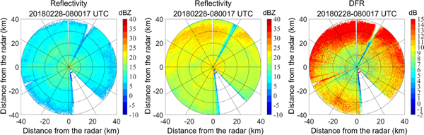
The most intense case during ICE-POP 2018 was on February 28th, 2018. During this event, the changes in precipitation phases varied from rain and then to snow. We focus on snow QPE, so the data from 08:00 UTC to 16:00 UTC were used for comparisons between the radar and gauges. Figure 2 shows D3R Ku-band and Ka-band observations of Z and DFR at an elevation angle of 4.8° at 08:00 UTC, February 28th, 2018.

3. Snowfall estimation algorithm

3.1 Estimation of density

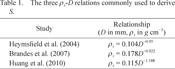
The snow density plays a major role in the estimation of snowfall rate (S), IWC, and linking microphysical parameters to polarimetric radar measurements. Unlike the density of raindrops, the snow density is not a constant and depends on many factors, including snowfall types and stages, as well as the climatological location. Because of this, the estimation of snowfall rate gets complex. The conventional method uses a power–law relation between the density and size (Table 1) (Brandes et al. 2007; Heymsfield et al. 2004; Huang et al. 2010). Heymsfield et al. (2004) used in situ aircraft measurements, the equation from Brandes et al. (2007) is based on 2DVD and the snow gage data from Colorado, and USA and Huang et al. (2010) used 2DVD and radar measurements to derive these equations. These relationships are all statistical relations and are derived using various datasets, reporting only the mean values. However, these relationships may not describe the events captured during ICE-POP 2018 well because the Pyeongchang Olympic region has a coastal climate and there are lots of water vapor coming from the ocean to affect the formation of the snowflakes. Furthermore, the temperature was −0.4°C, and the humidity was 97 % at the radar site at 12:00 UTC, February 28th, 2018. Therefore, the snow density in these oceanic climates is larger than that of the continental climate. Although the snow density could not be directly measured using the disdrometer, this study uses the terminal velocity and diameter measured by the disdrometer to indirectly get an idea of the snow density from which S is estimated.

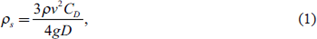
Ignoring the buoyancy, pressure gradient, and inertial forces, when gravitational force equals the drag force, the hydrometeor falls relative to the air at its terminal fall speed (Rogers and Yau 1989). The density can be approximated using velocity and diameter; this can be obtained using the disdrometer measurements and the equation below.   

where ρ is the density of air, v and D represent the velocity and median volume diameter measured by disdrometer, respectively, C_D is the drag coefficient, and g is the acceleration of gravity. After getting the velocity and diameter measured from 32 bins of Parsivel every minute, the snow density in every bin can be obtained according to Eq. (1).

Figure 3 shows the scatter density plot for diameter versus velocity taken on February 28th, 2018 at the YPO, CPO, and DGW sites. It can be seen from the Fig. 3 that the empirical terminal velocity of snow (red line) from Brandes et al. (2007) does not fit well for the disdrometer measurements. Most of the measured velocities of the snow particles during this event are larger than the velocities using Brandes' density relation.

Fig. 3.

Scatter density plot for diameter versus velocity for data measured on February 28th, 2018. The red line is empirical terminal velocity of snow from Brandes et al. (2007).

Figure 4 shows the plot of diameter versus density derived using disdrometer data from Eq. (1). The empirical ρ_s-D relations from Table 1 are also plotted with solid lines of different colors. None of the empirical equations describe the snow density during this event well. It can be seen from these figures that density retrieval is a challenge.

Fig. 4.

Plot of diameter versus density derived from disdrometer measurements. The solid lines indicate the three ρ_s-D relations from the literature. Red line is from Huang et al. (2010). Blue line comes from Heymsfield et al. (2004). Green line stems from Brandes et al. (2007).

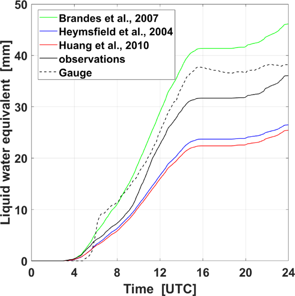
In order to demonstrate that the method used here to compute the snow density is more accurate than using empirical ρ_s-D relations from Table 1, we used the computed density determined by the disdrometer and empirical equations to calculate the snowfall rate. We then used these results to obtain the accumulations during this event and compared them with precipitation gage. Figure 5 shows the results of accumulation using three ρ_s-D relations and gage. The accumulation agrees well with the gauge after calculating density from the measured fall speed and diameters. Using relations from Brandes et al. (2007) overestimates accumulation, and using relations from Heymsfield et al. (2004) and Huang et al. (2010) underestimates accumulations. This shows that if we use the relationships from literature to derive the snow density and derive snowfall rate, it may result in errors.

Fig. 5.

Comparison of accumulations at the YPO site using ρ_s-D relations and gauge on February 28th, 2018.

3.2 Snowfall rate estimation

After determining the snow density, the reflectivity factor at the Ka- and Ku-band can be calculated from snow PSD as   

where λ is the wavelength of the radar, K_w is the dielectric factor of water, and σ_h is the radar cross section, which is calculated using the scattering model. For ice particles, scattering simulation is difficult because of their irregular shapes. Although the discrete dipole approximation can be used to simulate their scattering (Draine and Flatau 1994; Yurkin and Hoekstra 2011), it is time-consuming, and we need to construct their shapes. In radar meteorology, the T-matrix method is commonly used, but we need to simplify the snow particle to a spheroid. Garrett et al. (2015) found that the axis ratio of snow particles is between 0.6 and 0.7 by analyzing the observations from a multiple-angle snow camera. We regarded the axis ratio of snow particles with 0.7 and Gaussian canting angle distribution with a mean of zero and a 45° standard deviation. As for the refractive index of ice, we utilized the tables of Warren and Brandt (2008) at a temperature of 266 K, and they are 1.7861 + 3.116 × 10⁻⁴i and 1.7861 + 7.987 × 10⁻⁴i for the Ku- and Ka-band, respectively. Then, we used the Maxwell–Garnet mixture formula and the refractive index of ice to get the dielectric factor of snow in this paper.

The liquid water equivalent snowfall rate (S) in mm h⁻¹ for a 1-min time interval is defined using the equation below.   

In this equation, ρ_s is the snow density in g cm⁻³, which is calculated using Eq. (1) and the velocities and diameters measured using the disdrometer. N(D) is measured snow PSD (mm⁻¹ m⁻³), and D and v(D) are the measured diameter (mm) and velocity (m s⁻¹), respectively.

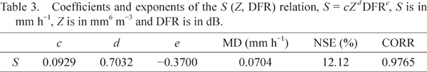
Once Z and S are obtained, we can fit power–law relation with the form S = aZ^b by using weighted total least square (WTLS) and S = cZ^d DFR^e by using non-linear least squares fitting (NLSF), and we used the Z at the Ku-band here. Note that the units of Z and S are mm⁶ m⁻³ and mm h⁻¹, respectively. The coefficients and exponents of two relations are given in Tables 2 and 3. In order to evaluate their errors, the mean difference (MD), normalized standard error (NSE), and correlation coefficient (CORR) are calculated, which are defined as   

  

  

where R_n and G_n denote S from the power–law and disdrometer-derived S, N is the total number of samples, NSE is in percentage, CORR is dimensionless, MD is in mm h⁻¹ here, and MD is in millimeters when we compare radar snowfall estimation with gauges in the next section.

Figure 6 shows the scatterplot of disdrometer-derived Z and S. The S-Z power–law fitting is overlaid on the scatterplot. The fitting uses the WTLS, and its NSD is 20.10 %. The scatterplots of snowfall rates from the relationships (S-Z and S-Z-DFR) computed and directly estimated using the disdrometer are displayed in Fig. 7. From the figure, we can see a very good match between the S estimated from the relationships and S derived from the disdrometer. It is obvious from Fig. 7, Tables 2, and 3 that the S (Z, DFR) performs well because it has a lower NSE of 12.12 % compared with the S (Z) method.

Fig. 6.

Scatterplot of Z vs. S derived from the disdrometer together with the S-Z power–law fitting.

Fig. 7.

Scatterplots of S (disdrometer) vs. S (Z) (red dots), and S (disdrometer) vs. S (Z, DFR) (black dots).

4. Results and discussion

In order to evaluate the performance of the two algorithms for snow QPE estimation, we have made comparisons between radar estimations and observations of precipitation gauges. The gauges measure accumulation with a resolution of 0.01 mm and represent point measurements. For radar, it measures the instantaneous snowfall rate and observes a large area, and its measurements are averaged for each resolution volume. The elevation of D3R radar scans were 4.8° and the time resolution was 5 min. The disdrometers and gauges are not far from the radar, so we chose the second range resolution at the YPO site and the forth range bin of the radar measurements to represent the radar measurement, respectively. There are the gauge and the D3R radar at the DGW site, so we averaged the reflectivity factor over all azimuthal beams at a 600-m range in the PPI scan. The accumulation for the YPO and CPO sites from the D3R data is obtained by first selecting the range and azimuth corresponding to the location of the gauge site. Then, the S is computed for that particular range resolution bin, and finally, the accumulation is computed for the required time interval.

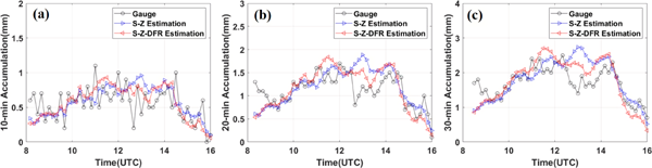
For snowfall measurements, snow particles tend to have a slower falling velocity and smaller accumulation every minute compared with rainfall, so we computed the accumulations in a 10-min resolution window to decrease the instability of measurements, which means we added S every two scans to derive S every 10 min. In order to analyze the temporal resolution effect on the accuracy of snowfall measurements, we aggregated the snowfall measurements to a 20- and 30-min scale. In this paper, we used the measurements of gauges as baselines for comparison with radar estimates using S-Z and S-Z-DFR algorithm. Figure 8 shows the plots of the 10-min, 20-min, and 30-min snowfall measurements using two algorithms from D3R radar data and gauge for the case of February 28th, 2018. From the figure, it can be seen that the accumulation obtained using the relationships match well with the gauge accumulation. Figures 9 and 10 show the comparisons of accumulation obtained from D3R radar data and gauge at the location of the CPO and DGW, respectively. The results at these locations also show a good match between the estimated and gauge accumulation.

Fig. 8.

Snowfall estimation using S-Z and S-Z-DFR algorithm from D3R radar and gauge at the YPO site on February 28th, 2018 when the timescale is, (a) 10-min, (b) 20-min, and (c) 30-min.

Fig. 9.

Snowfall estimation using S-Z and S-Z-DFR algorithm from D3R radar and gauge at the CPO site on February 28th, 2018 when the timescale is, (a) 10-min, (b) 20-min, and (c) 30-min.

Fig. 10.

Snowfall estimation using S-Z and S-Z-DFR algorithm from D3R radar and gage at the DGW site on February 28th, 2018 when the timescale is, (a) 10-min, (b) 20-min, and (c) 30-min.

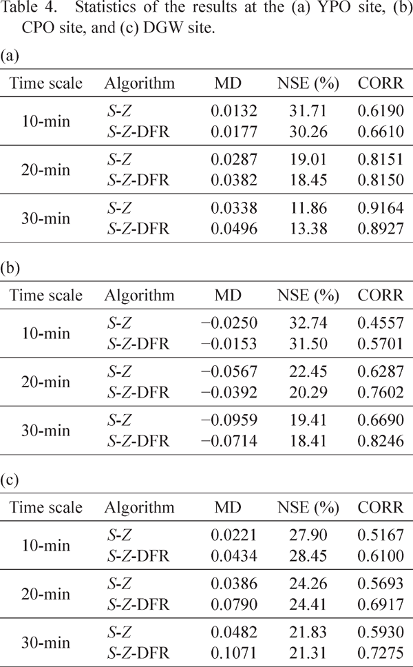
Next, we computed the statistics for the estimated accumulation. Table 4 shows the results of MD, NSE, and CORR using S-Z and S-Z-DFR estimation at the YPO, CPO, and DGW sites with respect to the gauge accumulation. It is obvious that the radar estimations using two algorithms agree with the observations from the gauges very well. It can also be seen that NSE decreases greatly as the snowfall accumulation scale time is increased from 10 min to 30 min. In addition, most NSE of the S-Z estimation is larger than that of the S-Z-DFR estimation. Going from 10 min to 30 min accumulation at the YPO site, NSE is reduced from 31.71 % to 11.86 % using S-Z estimation and from 30.26 % to 13.38 % using S-Z-DFR estimation. At the CPO site, NSE is reduced from 32.74 % to 19.41 % using S-Z estimation and from 31.50 % to 18.41 % using S-Z-DFR estimation. Finally, at the DGW site, NSE is reduced from 27.90 % to 21.83 % using S-Z estimation and from 28.45 % to 21.31 % using S-Z-DFR estimation. From these results, we can infer that the results from S-Z-DFR estimation have a smaller NSE and higher CORR than those of S-Z estimation.

5. Summary

Previous studies have developed S-Z relationships for snowfall estimation using disdrometers and radars. However, it is uncommon to use DFR to retrieve snowfall rate and evaluate the products. The main goal of this paper is to develop methods for snow estimation using D3R radar in a coastal area and evaluate their snowfall accumulation performance at different time scales. The case study chosen is from a strong snow event on 28th February, 2018 during the ICE-POP 2018 campaign in South Korea. We have considered Parsivel disdrometers at three sites (YPO, CPO, and DGW) to derive the relationships of S-Z and S-Z-DFR methods, which are then used to retrieve the snowfall rate.

One reason that snowfall is difficult to estimate is the diversity of the snow density. In prior works, power–law relationships between density and diameter are used to obtain the snow density, but they are not enough to describe the snow density because of different snow types and climatological locations. In this study, we used the velocity and diameter measured by the disdrometer to derive the snow density directly. It has been shown that using this method to obtain the snow density is more accurate than using conventional relationships. We used the obtained snow density to derive liquid water equivalent snowfall rate and equivalent radar reflectivity factor. The radar reflectivity factor is computed using the T-matrix method at the Ku- and Ka-band, which assumes that the axis ratio of snow is 0.7. Two relationships (S-Z and S-Z-DFR) to retrieve the snowfall rate are then determined, which is based on WTLS and NLSF, respectively.

We used these two relations to estimate the snowfall rate. The NASA D3R radar data during ICE-POP 2018 were analyzed for retrieving the snowfall estimation products. The estimated products are then compared with the ground measurements from gauges. The results show that the radar snowfall estimation agrees well with the ground observations at the three sites. S-Z-DFR algorithm performs better compared with S-Z algorithm as it has a lower NSE and a higher CORR. NSE decreases and CORR increases greatly as the snowfall accumulation scale time increases from 10 min to 30 min. For instance, at the YPO site, the NSE of the S-Z algorithm are 31.71, 19.01, and 11.86 % for 10-, 20-, and 30-min snowfall accumulation, respectively, and they are 30.26, 18.45, and 13.38 % for S-Z-DFR algorithm, respectively. At the CPO site, the NSE of the S-Z algorithm are 32.74, 22.45, and 19.41 % for 10-, 20-, and 30-min snowfall accumulation, respectively, and they are 31.5, 20.29, and 18.41 % for the S-Z-DFR algorithm, respectively. As for the DGW site, the NSE of the S-Z algorithm are 27.90, 24.26, and 21.83 % for 10-, 20-, and 30-min snowfall accumulation, respectively, and they are 28.45, 24.41, and 21.31 % for the S-Z-DFR algorithm, respectively.

Two snowfall rate estimation algorithms developed here could be used to estimate the snowfall in a similar coastal area. This is because they have similar environmental conditions such as the influence of the ocean and large snow density compared with inland regions. Moreover, these two algorithms indicate that using DFR to retrieve snowfall is a promising way and can be used as a ground validation tool for GPM snowfall production evaluations. However, more snow data should be collected and analyzed further.

Acknowledgments

The authors are greatly thankful to the participants of the World Weather Research Program Research Development Project and Forecast Demonstration Project, International Collaborative Experiments for Pyeongchang 2018 Olympic and Paralympic winter games (ICE-POP 2018), hosted by the Korea Meteorological Administration. D3R radar data were provided by the National Aeronautics and Space Administration (NASA) Global Hydrology Resource Center DAAC, Huntsville, Alabama, U.S.A. DOI: http://dx.doi.org/10.5067/GPMGV/ICEPOP/D3R/DATA101. The authors thank the Korean Meteorological Administration (KMA) for providing disdrometer and gauges data. One of the authors, Tiantian Yu, was supported by the China Scholarship Council. Tiantian Yu and Hui Xiao were also supported by the National Key Research and Development Plan of China (Grant Nos. 2016YFE0201900-02, 2019YFC1510304) and the National Natural Science Foundation of China (Grant No. 41575037). Two of the authors V. Chandrasekar and S. Joshil were supported by the NASA GPM-GV program.

References

•  Battaglia,  A.,  E.  Rustemeier,  A.  Tokay,  U.  Blahak, and  C.  Simmer, 2010: PARSIVEL snow observations: A critical assessment. J. Atmos. Oceanic. Technol., 27, 333-344.
•  Beauchamp,  R. M.,  V.  Chandrasekar,  H.  Chen, and  M.  Vega, 2015: Overview of the D3R observations during the IFloodS field experiment with emphasis on rainfall mapping and microphysics. J. Hydrometeor., 16, 2118-2132.
•  Brandes,  E. A.,  K.  Ikeda,  G.  Zhang,  M.  Schönhuber, and  R. M.  Rasmussen, 2007: A statistical and physical description of hydrometeor distributions in Colorado snowstorms using a video disdrometer. J. Appl. Meteor. Climatol., 46, 634-650.
•  Bukovčić,  P.,  A.  Ryzhkov,  D.  Zrnić, and  G.  Zhang, 2018: Polarimetric radar relations for quantification of snow based on disdrometer data. J. Appl. Meteor. Climatol., 57, 103-120.
•  Chandrasekar,  V., 2019: Indicate subset. GPM Ground Validation Dual-frequency Dual-polarized Doppler Radar (D3R) ICE POP [indicate subset used]. Dataset available online from the NASA Global Hydrology Resource Center DAAC, Huntsville, Alabama, U.S.A. [Available at https://dx.doi.org/10.5067/GPMGV/ICEPOP/D3R/DATA101.]
•  Cortinas,  J. V.,  B. C.  Bernstein,  C. C.  Robbins, and  J. W.  Strapp, 2004: An analysis of freezing rain, freezing drizzle, and ice pellets across the United States and Canada: 1976–1990. Wea. Forecasting, 19, 377-390.
•  Draine,  B. T., and  P. J.  Flatau, 1994: Discrete dipole approximation for scattering calculations. J. Opt. Soc. Amer. A, 11, 1491-1499.
•  Eriksson,  P.,  R.  Ekelund,  J.  Mendrok,  M.  Brath,  O.  Lemke, and  S. A.  Buehler, 2018: A general database of hydrometeor single scattering properties at microwave and sub-millimetre wavelengths. Earth Syst. Sci. Data, 10, 1301-1326.
•  Garrett,  T. J.,  S. E.  Yuter,  C.  Fallgatter,  K.  Shkurko,  S. R.  Rhodes, and  J. L.  Endries, 2015: Orientations and aspect ratios of falling snow. Geophys. Res. Lett., 42, 4617-4622.
•  Gehring,  J.,  A.  Oertel,  É.  Vignon,  N.  Jullien,  N.  Besic, and  A.  Berne, 2020: Microphysics and dynamics of snowfall associated with a warm conveyor belt over Korea. Atmos. Chem. Phys., 20, 7373-7392.
•  Hassan,  D.,  P. A.  Taylor, and  G. A.  Isaac, 2017: Snowfall rate estimation using C-band polarimetric radars. Meteor. Appl., 24, 142-156.
•  Heymsfield,  A. J.,  A.  Bansemer,  C.  Schmitt,  C.  Twohy, and  M. R.  Poellot, 2004: Effective ice particle densities derived from aircraft data. J. Atmos. Sci., 61, 982-1003.
•  Huang,  G.-J.,  V. N.  Bringi,  R.  Cifelli,  D.  Hudak, and  W. A.  Petersen, 2010: A methodology to derive radar reflectivity-liquid equivalent snow rate relations using C-band radar and a 2D video disdrometer. J. Atmos. Oceanic Technol., 27, 637-651.
•  Huang,  G.-J.,  V. N.  Bringi,  D.  Moisseev,  W. A.  Petersen,  L.  Bliven, and  D.  Hudak, 2015: Use of 2D-video disdrometer to derive mean density-size and Ze-SR relations: Four snow cases from the light precipitation validation experiment. Atmos. Res., 153, 34-48.
•  Huang,  G.-J.,  V. N.  Bringi,  A. J.  Newman,  G.  Lee,  D.  Moisseev, and  B. M.  Notaroš, 2019: Dual-wavelength radar technique development for snow rate estimation: A case study from GCPEx. Atmos. Meas. Tech., 12, 1409-1427.
•  Le,  M., and  V.  Chandrasekar, 2012: Raindrop size distribution retrieval from dual-frequency and dual-polarization radar. IEEE Trans. Geosci. Remote Sens., 50, 1748-1758.
•  Le,  M., and  V.  Chandrasekar, 2014: An algorithm for dropsize distribution retrieval from GPM dual-frequency precipitation radar. IEEE Trans. Geosci. Remote Sens., 52, 7170-7185.
•  Leinonen,  J.,  D.  Moisseev,  V.  Chandrasekar, and  J.  Koskinen, 2011: Mapping radar reflectivity values of snowfall between frequency bands. IEEE Trans. Geosci. Remote Sens., 49, 3047-3058.
•  Liao,  L., and  R.  Meneghini, 2019a: A modified dual-wavelength technique for Ku- and Ka-band radar rain retrieval. J. Appl. Meteor. Climatol., 58, 3-18.
•  Liao,  L., and  R.  Meneghini, 2019b: Physical evaluation of GPM DPR single- and dual-wavelength algorithms. J. Atmos. Oceanic Technol., 36, 883-902.
•  Liao,  L.,  R.  Meneghini,  A.  Tokay, and  H.  Kim, 2020: Assessment of Ku- and Ka-band dual-frequency radar for snow retrieval. J. Meteor. Soc. Japan, 98, 1129-1146.
•  Lu,  Y.,  Z.  Jiang,  K.  Aydin,  J.  Verlinde,  E. E.  Clothiaux, and  G.  Botta, 2016: A polarimetric scattering database for non-spherical ice particles at microwave wavelengths. Atmos. Meas. Tech., 9, 5119-5134.
•  Matrosov,  S. Y.,  M.  Maahn, and  G.  de Boer, 2019: Observational and modeling study of ice hydrometeor radar dual-wavelength ratios. J. Appl. Meteor. Climatol., 58, 2005-2017.
•  Rogers,  R. R., and  M. K.  Yau, 1989: A Short Course in Cloud Physics. 3rd Edition. Butterworth-Heinemann, 304 pp.
•  Souverijns,  N.,  A.  Gossart,  S.  Lhermitte,  I. V.  Gorodetskaya,  S.  Kneifel,  M.  Maahn,  F. L.  Bliven, and  N. P. M.  van Lipzig, 2017: Estimating radar reflectivity-Snowfall rate relationships and their uncertainties over Antarctica by combining disdrometer and radar observations. Atmos. Res., 196, 211-223.
•  Tyynelä,  J., and  V.  Chandrasekar, 2014: Characterizing falling snow using multifrequency dual-polarization measurements. J. Geophys. Res.: Atmos., 119, 8268-8283.
•  von Lerber,  A.,  D.  Moisseev,  L. F.  Bliven,  W.  Petersen,  A.-M.  Harri, and  V.  Chandrasekar, 2017: Microphysical properties of snow and their link to Ze-S relations during BAECC 2014. J. Appl. Meteor. Climatol., 56, 1561-1582.
•  Waliser,  D. E.,  J.-L. F.  Li,  C. P.  Woods,  R. T.  Austin,  J.  Bacmeister,  J.  Chern,  A.  Del Genio,  J. H.  Jiang,  Z.  Kuang,  H.  Meng,  P.  Minnis,  S.  Platnick,  W. B.  Rossow,  G. L.  Stephens,  S.  Sun-Mack,  W.-K.  Tao,  A. M.  Tompkins,  D. G.  Vane,  C.  Walker, and  D.  Wu, 2009: Cloud ice: A climate model challenge with signs and expectations of progress. J. Geophys. Res., 114, D00A21, doi:10.1029/2008JD010015.
•  Warren,  S. G., and  R. E.  Brandt, 2008: Optical constants of ice from the ultraviolet to the microwave: A revised compilation. J. Geophys. Res., 113, D14220, doi:10.1029/2007JD009744.
•  Yurkin,  M. A., and  A. G.  Hoekstra, 2011: The discrete-dipoleapproximation code ADDA: Capabilities and known limitations. J. Quant. Spectrosc. Radiat. Transfer, 112, 2234-2247.
•  Zhang,  G.,  S.  Luchs,  A.  Ryzhkov,  M.  Xue,  L.  Ryzhkova, and  Q.  Cao, 2011: Winter precipitation microphysics characterized by polarimetric radar and video disdrometer observations in central Oklahoma. J. Appl. Meteor. Climatol., 50, 1558-1570.