Abstract
The evolution of a heavy rainfall event that occurred on 19 August 2014 in northern Taiwan is investigated using observed data and analyzed using a newly developed system, namely, IBM_VDRAS. This system is based on a four-dimensional (4D) Variational Doppler Radar Assimilation System (VDRAS) that is capable of assimilating radar observations and surface station data over a complex terrain by adopting the Immersed Boundary Method (IBM). This event has precipitating processes and track different from those frequently observed in northern Taiwan.
From the surface observations and the high spatiotemporal resolution analysis fields generated by IBM_VDRAS, it has been found that the rainfall process started with two single convective cells triggered by the interaction between land–sea breeze and terrain in two different cities (Taoyuan and Taipei). The outflow of one of the convective cells developed in Taoyuan City at an earlier time along with the outflow of another convective system that developed in the Taipei Basin; the former provided favorable conditions to intensify the latter. The enhanced major convective cell moved to the Taipei City metropolitan area and produced 80-mm precipitation within approximately 2.5 h. The kinematic, thermodynamic, and microphysical fields of the convective cells were analyzed in detail to explain the mechanisms that helped maintain the structure of the rainfall system. Sensitivity experiments of quantitative precipitation forecast revealed that the terrains prevent the location of major rainfall from shifting outside of the Taipei Basin. By assimilating the surface data, the model can better predict the rainfall position.
1. Introduction
Taiwan is an island located in the subtropical zone of the Northwestern Pacific Ocean (Fig. 1). According to the official record released by the Water Resources Agency of Taiwan, the annual accumulated rainfall, mainly contributed by the seasonal Mei-Yu front, southwesterly flow, tropical cyclones, and afternoon thunderstorms, can reach as high as 2500 mm (https://eng.wra.gov.tw/7618/7664/7718/7719/7720/12622/). The torrential rainfall associated with these events may lead to flooding and compound disasters. Among them, the development of afternoon thunderstorms is closely related to the land–sea breezes and is affected by the island's complex terrain (Chen et al. 2014; Miao and Yang 2020). The afternoon thunderstorms are characterized by their short lifespan, small scale, strong intensity, and multiple convective cells. The nonlinear interaction among convective cells, some of which are very short-lived, helps prolong the lifetime of the thunderstorm and enhance the amount of rainfall. Furthermore, the terrain of Taiwan affects the flow fields, altering the location, scale and intensity of the precipitation, making forecast of the convection initiation, propagation, and intensification more complex. Understanding the mechanisms leading to the occurrence of afternoon thunderstorms is important for the improvement of forecasting and for disaster prevention.
Johnson and Bresch (1991) found that the afternoon convective activity in Taiwan often occurred between the 100- and 500-m elevations at the foothills of the mountains rather than over the higher elevations farther inland. Chen and Chen (2003) pointed out that with a pronounced diurnal heating cycle during the summer months, afternoon convective rainshowers are frequently observed along the windward side of the mountain in Taiwan. Lin et al. (2011) explored the characteristics of warm season (June to August) thunderstorms over Taiwan and demonstrated that thunderstorms mainly occurred on the windward side of the mountain range along the foothills (300–500-m height) when the sea breeze impinged upon the mountains. In northern Taiwan, particularly Taipei City, which is located in the Taipei Basin and is the political and economic center of Taiwan (see Fig. 2 for its location), most thunderstorm tracks run parallel to the orientation of the mountain range [i.e., Snow Mountain Range (SMR), to be introduced in Section 3.1]. The northerly winds in the Taipei Basin with warmer temperature and higher moisture than the climatological average are sufficient to trigger thunderstorms. The study of Chen et al. (2014) revealed that under weak synoptic forcing, 75 % of the rainfall in the Taipei Basin during the summer season can be attributed to afternoon thunderstorm, which was induced by sea breeze interactions with the mountains to the south of the basin.
From an observational perspective, Malkus (1954), Malkus and Riehl (1964), Simpson et al. (1971), Westcott (1984), and Simpson et al. (1993) revealed that cell merging may expand the horizontal coverage and the lifecycle of a storm system and thus intensify the rainfall. Using model simulations, Tao and Simpson (1984, 1989) pointed out that the nonlinear interaction between the cold pool outflows originating from the convective downburst is the dominant physical process during cell merging. The clouds formed by the collision between cold pools bridge the adjacent convective systems. Feng et al. (2015) suggested that interacting cold pools trigger more convective cells than isolated ones due to the intensification of low-level convergence when the cold pools collide. In addition, the cold pools may expand the humid environment and decrease dry-air entrainment, which turn out to be favorable conditions for heavy rainfall. In Taiwan, Jou et al. (2016) analyzed the case of a thunderstorm that occurred on 14 June 2015 in Taipei City using radar and surface station observations. They also observed a cell merging process followed by heavy rainfall. This particular severe rainfall event was further investigated by Miao and Yang (2020) using numerical model simulations. They described the cell merging process and investigated the role played by sea breeze, terrain, and evaporative cooling effect.
Efforts to predict afternoon thunderstorm during the warm season in Taiwan can be found in the study by Lin et al. (2012) in which pre-convective predictors derived from surface stations and sounding measurements were used. Chen, T.-C. et al. (2016) utilized the primary features of the synoptic conditions and timings of the diurnal cycles for pressure, temperature, dew point depression, and relative humidity observed by surface stations to develop a two-step hybrid forecast advisory for the occurrence of summer afternoon thunderstorm in the Taipei Basin. Chang et al. (2017) reported that the fuzzy-logic-based nowcasting system operated by the Central Weather Bureau of Taiwan has moderate accuracy. This system generated 1-h likelihood nowcasts of afternoon convection initiation and was found to outperform operational hot-start numerical weather prediction models.
A Doppler weather radar is a powerful remote-sensing instrument that can provide 3D high spatiotemporal resolution observations of the severe weather systems. However, the meteorological data collected by each instrument only give some part of the information on the weather. Hence, efforts have been made in data assimilation to optimally merge the data obtained from model outputs and various types of observations in order to achieve the best and complete description of the atmospheric status. For example, due to the curvature of the Earth and radar scanning strategies, the radar cannot observe the atmosphere at lower levels. Thus, the data measured by surface stations become useful in terms of providing information for the data-void region near the ground. The products of a data assimilation system can be very useful for improving weather diagnosis and forecasts.
Various types of data assimilation methods have been developed, such as the variational approach (including three- and four-dimensional variational data assimilation; hereafter, 3DVar and 4DVar, respectively), ensemble Kalman filter, and their hybrid (e.g., Snyder and Zhang 2003; Gao et al. 2004; Tong and Xue 2005; Xue 2006; Xiao and Sun 2007; Chung et al. 2009; Li et al. 2012; Gao et al. 2016; Pan et al. 2012; Xiao et al. 2017). In this study, the Variational Doppler Radar Analysis System (VDRAS; Sun and Crook 1997), which was originally developed at the National Center for Atmospheric Research, is utilized after further improvement. By assimilating the observations using the 4DVar technique, VDRAS is able to provide analysis fields with high spatiotemporal resolution (Chang et al. 2014, 2016). This system has been quite successful in numerous applications, ranging from basic research to operational utilization for special sporting events (e.g., Sun and Crook 2001; Crook and Sun 2002, 2004; Sun et al. 2010; Sun and Zhang 2008; Tai et al. 2011; Chang et al. 2016; Gochis et al. 2015; Friedrich et al. 2016; Xiao et al. 2017). Significant improvements were accomplished in the study by Tai et al. (2017) by implementing a terrain-resolving capability to VDRAS.
Although it has been well recognized, the thunderstorms in northern Taiwan often started to develop on the mountain peaks to the south of the Taipei Basin; then, they propagated northward along the terrain slope down to the Taipei City and produced heavy rainfall (Jou 1994; Chen et al. 2014). In this study, the newly developed VDRAS is used to investigate in detail the evolution of a heavy rainfall event that possesses precipitating processes and track different from those mentioned above, as well as the associated triggering and maintenance mechanisms. This event was a summer afternoon thunderstorm that occurred on 19 August 2014 in northern Taiwan.
The remainder of this manuscript is organized as follows. Section 2 briefly introduces the new VDRAS and the additional function for assimilating surface data. In Section 3, we provide an overview of the event, description of the experimental designs, model settings, and assimilation strategy. In Section 4, we present the evolution of the heavy rainfall event as revealed by surface observations and 4DVar analyses. The structure and maintenance mechanisms as well as the microphysical processes of this precipitation event are presented in Sections 5 and 6, respectively. In Section 7, sensitivity tests are conducted to investigate the impact of the topographic effect and surface data assimilation on the model performance in terms of the quantitative precipitation forecast (QPF). The results are summarized in Section 8.
2. A brief introduction of the 4DVar data assimilation system
2.1 IBM_VDRAS
Using the 4DVar technique, VDRAS obtains an optimal model initial condition from which the discrepancy between the model forecasts and observations within an assimilation cycle reaches a minimum. VDRAS is constrained by a cloud-resolving model and contains six prognostic equations: the three momentum equations, thermodynamic equation, rainwater equation, and total water equation. Tai et al. (2017) implemented VDRAS using the Immersed Boundary Method (IBM) proposed by Tseng and Ferziger (2003), allowing the orographic effect exerted on the fluid to be taken into account by performing forward and backward integrations of the forecast and adjoint model directly over the terrain. The new system that possesses this terrain-resolving capability is called IBM_VDRAS. After assimilating observational data, primarily from Doppler radars, IBM_VDRAS generates a series of high spatiotemporal resolution 3D model state variables including the wind and the thermodynamic and microphysical parameters over terrain. The unique feature of IBM_VDRAS is designed particularly for analyzing convective-scale weather and nowcasting (Tai et al. 2017).
2.2 Assimilation of surface data
The low-level atmospheric conditions are crucial for the initiation and evolution of convection but are usually difficult to observe by weather radar. Seto et al. (2018) revealed that in Tokyo, Japan, the surface wind convergence observed by high-density weather stations reached its peak 10–30 min prior to the occurrence of the heavy rainfall. Liou et al. (2019) demonstrated how to utilize the wind observations from surface stations to improve the analysis of the flow field within the boundary layer. In the original design of VDRAS, the surface observations were used only to construct the mesoscale background field (Crook and Sun 2002). In this study, a different approach is adopted by which IBM_VDRAS is modified so that the wind, temperature, and water vapor mixing ratio (qv; converted from relative humidity) measured by the surface stations can be directly assimilated during the minimization procedure.
The cost function with the surface observation terms implemented is expressed as follows:
The summation is performed over space (
x, y, z) and time (
t);
xo and
xb denote the initial state of the model variables and background fields, respectively, and
B denotes the background error covariance matrix.
ηv and
ηq are specified to be 1.0 and 50.0, respectively, so that the magnitude of each term can be balanced. These two coefficients control the extent to which the 4DVar algorithm minimizes the differences between the model-produced radar radial velocity (
Vr), rainwater mixing ratio (
qr), and their observed counterparts (i.e.,
Vor and
qor).
Jp stands for a penalty term for smoothing the resulting analysis fields, and
Jmb denotes the mesoscale background field, which in this study is obtained from the European Centre for Medium-Range Weather Forecast. The model-generated surface horizontal winds, temperature, and vapor are denoted by
us,
vs,
Ts, and
qv, s, respectively, whereas their observed counterparts from the surface stations are denoted by a superscript “o”. The constant values
ϕu,
ϕv,
ϕT, and
ϕqv are the weighting coefficients for surface assimilation, which are assigned values of 1.0 in this study after a series of sensitivity tests to find the optimal values. It should be noted that the first four terms on the right-hand side of
Eq. (1) are from the original VDRAS.
Usually, surface stations are not located precisely at the model grid points. Therefore, the surface observations, including those measured by mountain stations, are first shifted horizontally to the nearest position right below (or above) a model grid point. Then, the wind measurements are extrapolated vertically to the model grid points through a power law (Peterson and Hennessey 1978), whereas the temperature and vapor data are extrapolated following a vertical profile obtained by making a horizontal average of the mesoscale background field. Finally, the Barnes (1964) objective analysis scheme is employed to distribute the observed information to the surrounding grid points located on the same horizontal plane. It should be noted that Chen, X. et al. (2016) reported on the assimilation of surface wind and temperature data to improve the analysis and forecast ability of VDRAS. However, in our design, the water vapor measurements from the surface stations are also assimilated along with the temperature and winds. In addition, the data collected by mountain stations are also fully used by our IBM_VDRAS.
The strategy adopted in this study is the utilization of the wind and temperature observed by surface stations to provide information regarding the initiation of convection before the radars can detect any significant signals prior to the development of convective cells. In addition, the accumulated rainfall measured by rain gauges is used to understand the precipitation pattern and magnitude of this event during the entire episode. When more radar data are available as the convective system begins to develop, the analysis fields generated by IBM_VDRAS, including 3D winds, temperature, rainwater mixing ratio, water vapor flux, and microphysical processes (i.e., accretion, autoconversion, and evaporation), are applied to study the subsequent rainfall processes and mechanisms. It should be noted that the analysis fields are outputs from IBM_VDRAS after the assimilation of radar data and wind, temperature, and vapor measured by surface stations, as indicated by the cost function presented in Eq. (1).
3. Introduction of the event and experimental designs
3.1 An overview of the event and deployment of radars
The selected event for this study occurred on 19 August in 2014, and it was a summer afternoon thunderstorm in northern Taiwan. The 850-hPa weather chart based on the data from ECMWF at 08:00 LST (00:00 UTC) on 19 August 2014 (Fig. 1) reveals that the prevailing synoptic scale flow was mainly southerly, which could transport moisture toward Taiwan from the warm ocean prior to the development of the thunderstorms. The sounding released in northern Taiwan at 14:00 LST (not shown) demonstrates that the value of the convective available potential energy exceeded 2,250 m2 s−2, indicating favorable conditions for the formation of storms once the convection reaches the level of free convection at Z = 1.05 km.

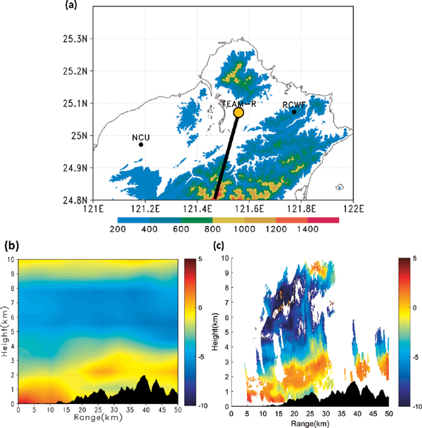
The analysis domain presented in Fig. 2 ranges from 24.8°N to 25.4°N and from 121°E to 122°E. The topography includes Taipei City, the Taipei Basin, Taoyuan City, Linkou Highland (LKHL), Mountain Yangming (MTYM), and the SMR. The LKHL, MTYM, and SMR are about 200, 1,000, and 1,400 m high and situated to the west, north, and south of the Taipei Basin, respectively. The Tamsui River and Keelung River, originating from the SMR, flow northwest and northeast through the Taipei Basin, respectively.
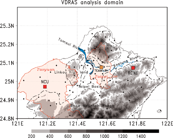
The locations of three radar systems are also marked in Fig. 2. They include RCWF (25.07°N, 121.77°E, height: 770 m), an S-band radar operated by the Central Weather Bureau (CWB) of Taiwan with a maximum observational distance of 230 km; the NCU radar (24.97°N, 121.18°E, height: 158 m), a C-band radar operated by the National Central University (NCU) with a maximum observational distance of 125 km; and TEAM-R (25.08°N, 121.56°E, height: 0 m), an X-band mobile radar also operated by NCU. Both the RCWF and NCU radars conducted volume scans containing nine scanning angles (0.5, 1.5, 2.4, 3.4, 4.3, 6.0, 9.9, 14.6, and 19.5) and can output the reflectivity (ZH), Doppler velocity (Vr), spectrum width, and dualpolarization variables. The quality control procedure includes the removal of the non-meteorological signals (e.g., ground clutter and sea clutter), unfolding of the radial velocity, and data interpolation.
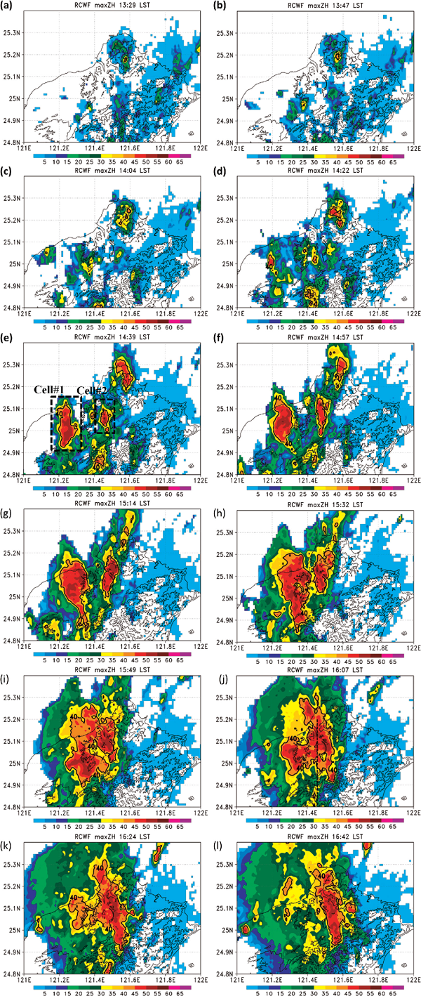
Figure 3 presents a sequence of composite radar reflectivity observed by the RCWF radar from 13:29 to 16:42 LST. It can be seen from the figure that multiple convective cells developed during this event. Figures 3a–f present the growth of the major reflectivity at Taoyuan City, followed by the development of convective cells in the Taipei Basin. The convection developed north of MTYM (see Fig. 3d), propagated to the north, and then dissipated later, thus not causing any damage. Using 40-dBZ radar reflectivity to define the boundaries of the convective cells, the first two cells labeled as cell #1 and cell #2 are identified in Fig. 3e. These two convective cells intensified until they finally merged into one NNW-SSE-oriented convection band (Figs. 3g–i), producing heavy precipitation in Taipei City (Figs. 3j–l).
3.2 Experimental settings, assimilation strategy, and verification
The IBM_VDRAS grid has a spatial resolution of 1.0 km and 0.25 km in horizontal and vertical directions, respectively, with the number of grid points being 150 and 100 along the west–east and south–north directions to cover the analysis domain presented in Fig. 2. The domain's vertical dimension contains 60 layers, from 0.125 km to 14.875 km in height. It should be noted that IBM_VDRAS is applied to assimilate the radial wind and reflectivity from the RCWF and NCU radars and the temperature, surface wind, and relative humidity observed by 80 surface stations. The data from TEAM-R and the Taipei surface station (25.03°N, 121.51°E, located at the center of the domain) are not assimilated. Instead, they are used to verify the results yielded by IBM_VDRAS.
Figure 4 presents the assimilation procedure which lasts for about 2.5 h, from 14:27 to 16:42 LST. IBM_VDRAS is performed in continuous cycles, which means that, with the exception of the first assimilation cycle, the initial guess for each cycle is directly obtained from the model results at the starting time of each cycle. Each assimilation cycle lasts for approximately 12.5 min and assimilates data from three volumetric scans by the RCWF radar, at least one volumetric scan by the NCU radar, and surface station observations. A 5-min pure model integration period is inserted between two assimilation cycles to improve the accuracy, as suggested by Sun and Zhang (2008). The 3D meteorological variables at the end of each cycle are the analysis fields of the assimilation. In this study, eight analysis fields about 18-min apart were generated at 14:39, 14:57, 15:14, 15:32, 15:49, 16:07, 16:24, and 16:42 LST. This set of analysis fields with high spatial resolution over the complex terrain is used to investigate the convection structure and triggering mechanisms.

The TEAM-R radar deployed in the Taipei Basin (see Fig. 2) is used as an independent data source for verification. Figure 5 presents a comparison of the radial wind produced by IBM_VDRAS and that observed by the TEAM-R Range Height Indicator (RHI) scan at 14:39 LST. The analysis field reveals that the northerly wind just above the terrain and southerly wind at the mid- and high levels (4–8 km) are in good agreement with the TEAM-R observation, although the retrieved wind speed is smaller than the observations, due to the smoothing of the IBM_VDRAS fields.
The surface temperature observations from the Taipei surface station (see Fig. 2) are used to verify the IBM_VDRAS analysis. It is found that the temperature retrieved by IBM_VDRAS is closer to the Taipei station in situ observations after the assimilation of all surface station data (excluding the Taipei station). The maximum temperature difference between surface observations and analyses without the assimilation of surface data can exceed 3°C, whereas analysis with the assimilation of surface data reduces the difference to about 1°C or less throughout the period from 14:39 LST to 16:42 LST (not shown). This result suggests the necessity of surface data assimilation in improving the accuracy of the retrieved low-level atmospheric conditions.
4. Rainfall processes revealed by surface observations and IBM_VDRAS analyses
To carry out a complete discussion about the structure and evolution of the convective systems leading to the heavy rainfall event in the Taipei Basin, the surface station data alone are used before the convection initiation (i.e., pre-storm environment), whereas a series of frequently updated analysis fields retrieved by IBM_VDRAS after assimilating radar and surface station data are utilized after the development of convection.
4.1 Surface station analyses before the initiation of convection
From the analysis of surface station observations at 12:30 LST presented in Fig. 6a, it can be seen that surface heating is notable, especially in the Taipei Basin and the northwestern coastal area where the temperature can exceed 32°C. The temperature analysis presented in Figs. 6b and 6c shows a drop in the temperature with time in Taoyuan City. Interestingly, the radar did not detect any significant echo during this period of time, but the Multi-functional Transport Satellite imagery indicates that most of the Taoyuan City area was covered by cloud for a significantly long period (not shown). Thus, it is believed that the decrease in temperature after 12:30 LST is mainly caused by the blocking of solar radiation.
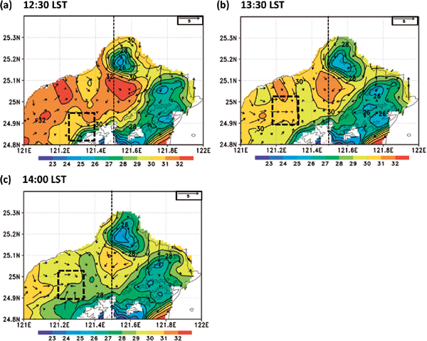
The sea breeze caused by the heating contrast between the ocean and land is significant along the coast line. Figure 6 shows that the winds in the domain east of 121.5°E during this 1.5-h period are mainly northerly and northeasterly, opposite to the synoptic southwesterly flow entering the analysis domain along the southwest boundary. The synoptic southwesterly flow, partially blocked by the SMR, collides with the northerly and northeasterly flows, leading to the formation of a convergence zone over the foothills on the western side of the SMR (see Fig. 7a). This convergence zone extends from the foothills to the plain area of Taoyuan City (indicated by the black dashed boxes in Figs. 6, 7), with a significant increase in intensity (Fig. 7). Conversely, the sea breeze also flows to the Taipei Basin along the Tamsui River and the Keelung River, forming a convergence zone in the basin. At 13:30 and 14:00 LST (Figs. 7b, c), a strong convergence zone can be identified approximately at (121.55°E, 24.95°N), located on the southern/northern side of the Taipei Basin/SMR due to the topographic blockage.

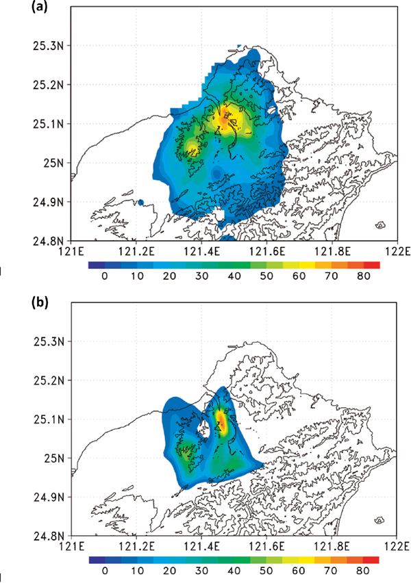
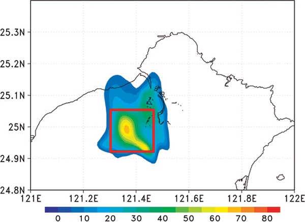
Observations of the rainfall which accumulated within the time period of eight data assimilation cycles are presented in Fig. 8. Figure 8a shows that from 14:22 to 14:39 LST, only minor rainfall (∼ 2 mm) occurs in the northern tip of the island. However, significant rainfall starts at 14:39 LST extending from the western side of the LKHL to the coast of Taoyuan City and on the eastern/western side of the LKHL/Taipei Basin, but with a lesser amount (see Fig. 8b). From Figs. 8c and 8d, two distinct rainfall regions are identified on the eastern and western sides of the LKHL. In a large portion of the rainfall area, the accumulated rainfall within a time period of 18 min is about 10 mm, which is equivalent to a rain rate of approximately 33 mm h−1. By comparing Figs. 8c and 8d with Fig. 8e, it is found that after 15:32 LST, the accumulated rainfall within the same time period of 18 min can reach 20 mm, indicating a dramatic increase in rainfall rate to 67 mm h−1. This rainfall intensity continues until 16:42 LST (see from Fig. 8e to Fig. 8h). Figures 8e to 8f show that along 121.4°E, the precipitation has two maxima, with the southern one disappearing only 20 min later. In Taoyuan City, the rainfall gradually dissipates after 16:07 LST. However, in the northern part of Taipei City, a rainfall maximum remains nearly stationary (Figs. 8e–h). Figure 9 reveals the accumulated rainfall (reaching 80 mm within approximately 2.5 h) in the Taipei Basin.

With more radar data becoming available for assimilation after 14:00 LST, the structure and evolution of this heavy rainfall event are further investigated by eight analysis fields generated by IBM_VDRAS. Figure 10 presents the horizontal wind, divergence, and vertical velocity, whereas the temperature perturbation (from a horizontal average) and relative humidity from selected time periods are presented in Fig. 11. Some of these fields are displayed over a terrain-following surface, which is defined as the first grid point immediately above the terrain.

The first IBM_VDRAS analysis was produced at 14:39 LST (Fig. 10a). At this moment, as presented in Fig. 3e, the radar observations detect two distinct convective cells located to the west and east of the LKHL and are labeled cell #1 and cell #2, respectively. In Fig. 10a, there is a significant convergence located to the west of the LKHL and south of the Taipei Basin. The vertical velocity field at 1.0 km above the ground presented in the same figure indicates that the locations of the updraft agree well with the low-level convergence throughout the entire analysis period. The temperature fields retrieved by IBM_VDRAS (Fig. 11a) clearly indicate that at 14:39 LST, both cells are associated with negative perturbations at a low level, implying that the cooling effect induced by evaporation is active. The structures of cells #1 and #2 are described in Figs. 12 and 13, in which the divergence, vertical velocity, streamlines, and rainwater mixing ratio along two north–south-oriented vertical cross sections penetrating these two cells (see Fig. 10a) are displayed. It can be seen from the figure that both cells are co-located with convergence below and divergence aloft. The maximum magnitudes and locations of the divergence are −2.0 × 10⁻³ s−1 at 1.0 km for cell #1 and −0.5 × 10⁻³ s−1 at 3.5 km for cell #2, respectively (Figs. 12a, 13a). The surface convergence in cell #2 is much weaker than that of cell #1. Furthermore, using the 1.0-m s−1 contour line as a boundary, the updraft in cell #1 develops to a higher altitude (8.0 km), with the maximum value reaching 7.0 m s−1. Contrarily, the weaker vertical air motion (∼ 2.0 m s−1) in cell #2 is confined to the area below Z = 5.0 km. Using 0.2 g kg−1 of rainwater mixing ratio as a threshold, cell #1 can grow up to 7.0 km, whereas cell #2 reaches only 4.5 km (Figs. 12b, 13b). With a much stronger lowlevel convergence, cell #1 is more upright and deeper than cell #2. The aforementioned information indicates that cell #1 reaches the mature stage earlier than cell #2.

Figure 10b shows that due to the terrain effect, a northeast–southwest-oriented convergence line is present along the northern boundary of the SMR with updraft. This convergence line persists for over 1 h from 14:57 LST to 16:07 LST, as presented from Fig. 10b to Fig. 10f. From 14:57 LST to 15:32 LST, the radar reflectivity presented in Fig. 3f to Fig. 3h indicates that both cells keep expanding and intensifying. This phenomenon is also confirmed by Figs. 11b–d, from which it can be seen that the temperature continues to decrease, and the area of negative temperature perturbations spreads with time. At the location of cell #1, the magnitude of the low-level divergence increases with time due to the cold air outflow (Figs. 10b–d; location is marked in Fig. 10c). The eastern branch of the outflow from cell #1 passes the LKHL and arrives at cell #2, providing additional convergence. The temperature drop in the cold outflow helps increase the relative humidity in the Taipei Basin (see Figs. 10c, d, 11c, d). A line of low-level convergence associated with updrafts forms on the eastern side of the LKHL between cell #1 and cell #2 at 15:32 LST (Fig. 10d), where a significant rainfall occurs as presented in Fig. 8e.
c. 15:32–16:42 LST
From 15:32 LST to 16:42 LST, the radar reflectivity presented in Figs. 3h–l indicates that two cells merge into one, which remains nearly stationary in the Taipei Basin area. Rainfall starts to dramatically accumulate during this period (Figs. 8e–h). This merged cell is associated with a roughly north–south-oriented low-level convergence line with embedded upward motion at the Taipei Basin (see Figs. 10d–h; location is marked in Figs. 10d, f). A further examination reveals that the low-level convergence is mainly attributed to the collision of easterly and westerly winds (not shown). A large area of divergence induced by the cold air outflow can also be identified surrounding the low-level convergence. As can be seen from Figs. 11d–f, the cold pool keeps strengthening, as the temperature perturbation decreases with time to below −3.5° at 16:42 LST.
After 16:24 LST, the persistent convergence line located along the northern boundary of SMR since 14:57 LST was finally pushed away by the strong outflow toward the east (see Figs. 10g, h).
5. The structure of the precipitating system and the maintenance mechanisms
As discussed in Section 4 and illustrated by the radar reflectivity in Figs. 3h–l, two cells merged into one after 15:32 LST, becoming nearly stationary over the Taipei Basin during the period from 15:32 LST to 16:42 LST. The greater part of the precipitation fell in the northern part of the basin (Fig. 9). The meteorological fields were simulated by IBM_VDRAS after 15:32 LST, with a temporal resolution of 10 min to describe in more detail the structure and maintenance mechanisms of this line-shaped rain band after the cell merging. In Fig. 14, the wind vector, convergence, cloud water mixing ratio (qc), and convergence of the water vapor flux are computed. The latter is defined as −∇ (ρqvV̄), where ρ denotes the air density and V̄, the wind vector. These fields are displayed on a north–south-oriented vertical cross section penetrating the Taipei Basin at 121.46°E (shown by a dashed line in Fig. 3j).
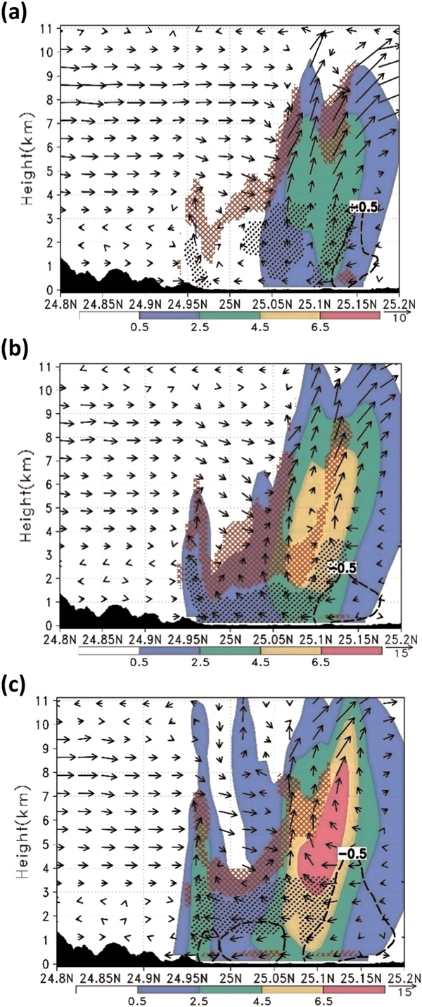
The north–south-oriented low-level convergence line presented in Fig. 10d is also obvious in Fig. 14a. The qr field significantly intensifies with time over a period of 20 min. A downward airflow can be observed below the main merged cell (see the broken contour lines at low levels near 25.15°N in Fig. 14a). The area with descending flow expands southward with time, as presented in Figs. 14b and 14c. The lowlevel outflow wind from this merged cell in the northern part of the Taipei Basin blows toward the south. When the flow reaches the SMR and is blocked, a low-level convergence zone is generated, triggering updraft and a new convective cell near 24.95°N (Figs. 14b, c). It should be noted that this convergence zone located in the northern side of SMR is also presented in Fig. 10b. The new convective cell grows to an altitude of about 6.5 km, where the persistent southerly wind can be found in mid to high layers. The negative divergence of water vapor flux, or water vapor convergence, can be identified from the location of the new cell in the south to the merged cell in the north, indicating that the local circulation in the Taipei Basin supports the transport of water vapor northward and helps maintain the merged cell. As a result, the main precipitation occurs in the northern part of the Taipei Basin.
6. The microphysical processes associated with the intensification of the convection
The major microphysical processes that govern the formation of rainwater in this event are examined as follows. In IBM_VDRAS, as discussed by Sun and Crook (1997) and Chang et al. (2016), the processes include the autoconversion of cloud to rain, accretion of cloud by rain, evaporation of rainwater in subsaturated air, and sedimentation. Our computation demonstrates that the sedimentation effect plays a minor role in this case, thus is not shown. From Fig. 15, it is realized that the main contributor to the formation of rainwater is accretion, followed by autoconversion. The evaporation is the dominant microphysical process at lower altitudes and surface and significantly amplifies with time. This is consistent with the increasingly strong negative temperature perturbation presented in Fig. 11.
7. Sensitivity studies for topographic effect and surface data assimilation
7.1 Rainfall forecasts by IBM_VDRAS
Numerical experiments are first conducted in which IBM_VDRAS generates forecast of the rainfall after completing the data assimilation cycles. Since IBM_VDRAS requires a sufficient number of assimilation cycles, the experiment starting from 15:32 LST after four continuous assimilation cycles (see Fig. 4) are completed and end at 17:02 LST is selected for the discussion of the rainfall forecasts. The observed rainfall signal for the Taipei Basin presented in Fig. 16a can be well captured by IBM_VDRAS, as presented in Fig. 16b. The accumulated rainfall over 90 min forecasted by IBM_VDRAS reaches 75 mm, which is comparable to the observations. Thus, this experiment, named “CTL”, is selected as the benchmark experiment to study the impact of the topographic effect and surface data assimilation on the rainfall forecast.
7.2 Sensitivity tests of the topographic effect
To investigate the influence of the topographic effect on the model QPF skill, we conduct the “NO_TER” experiment, in which all terrains are removed during the assimilation cycles and the subsequent 90-min forecast. Figure 17 shows that the location of maximum rainfall in NO_TER is shifted to the south of the LKHL (see the red box in Fig. 17), which is further southwest compared with the CTL results (Fig. 16b). Figure 18 presents the computation of the difference in the winds at 15:32 LST between CTL and NO_TER at Z = 375 m. The westerly wind component near the LKHL and the southwesterly wind component along the SMR (see red boxes in Fig. 18) indicate that the role played by the topographic effect is to enhance the winds in these regions, which helps maintain the location of the major rainfall inside the Taipei Basin.
7.3 Sensitivity tests of surface data assimilation
In this section, the impact of the assimilation of surface data on the QPF is explored. The experiments include the “RADAR_ONLY”, with only radar data incorporated in the assimilation cycles, and “SFC_UV”, “SFC_T”, and “SFC_QV”, in which the radar data are assimilated along with the surface wind, temperature, and relative humidity data, respectively. Furthermore, the “SFC_TQV”, “SFC_UVQV”, and “SFC_UVT” represent experiments which assimilate radar and all surface station data except the wind, temperature, and relative humidity data, respectively.
Figure 19 presents the QPF results for each experiment. The comparison of the observations and CTL run results (see Section 7.1 and Fig. 16b) reveals that although the maximum rainfall amount is comparable, the location of the major rainfall in RADAR_ONLY is further south (Fig. 19a). This indicates that the assimilation of only radar data can produce sufficient amount of rainfall, but there is an obvious positional error in this case. The SFC_T, SFC_QV, and SFC_TQV results all reveal a similar pattern, which is the occurrence of heavy rainfall in the southern part of the Taipei Basin. However, in SFC_UV, SFC_UVT, and SFC_UVQV, a significant correction of positional error is achieved. These experiments suggest that the assimilation of surface wind is the critical factor for improvement of QPF in this case study. It is also speculated that during the assimilation cycles, the surface humidity in the analysis domain is already nearly saturated due to the occurrence of the rainfall event; thus, the usefulness of assimilating humidity information is limited.

The impact of surface wind assimilation is further investigated by comparing the surface wind analysis fields at 15:32 LST obtained from RADAR_ONLY and SFC_UV (Figs. 19a, b). It can be seen that in experiment RADAR_ONLY, stronger northerly wind can be identified in the foothills of the SMR than that in SFC_UV. Without the adjustment using surface wind observations, the additional northerly wind component in RADAR_ONLY will make the convergence near the foothills of the SMR too strong, which results in an overestimation of the convection in the southern part of the Taipei Basin and an inaccurate rainfall distribution.
8. Summary
In northern Taiwan, the severe afternoon thunderstorms often occurred on the peaks of mountains located to the south of the Taipei Basin and then propagated northward along the terrain slope down to Taipei City. This study describes in detail the evolution of a heavy rainfall event which possesses precipitating processes and track different from those frequently observed, as mentioned above. The processes and maintenance mechanisms of this particular event that occurred on 19 August 2014 as well as the results of the sensitivity studies are summarized as follows:
-
(1) Due to surface heating contrast, the sea breeze flows to Taoyuan City and enters the Taipei Basin along the Tamsui River and the Keelung River (see Fig. 6).
-
(2) The SMR blocks the prevailing southwesterly winds and the sea breeze winds, causing two low-level convergence zones in the foothills of the SMR (see Fig. 7).
-
(3) The convergence core extends from the mountains to the plain area of Taoyuan City, where cell #1 starts to develop. Cell #2 starts to grow in the Taipei Basin (see Figs. 3e, 7c).
-
(4) With stronger low-level convergence, cell #1 intensifies in advance of cell #2 (see Figs. 12, 13).
-
(5) Cell #1 merges with cell #2 in the Taipei Basin. A stationary north–south-oriented convection line associated with low-level convergence forms from the north of the Taipei Basin to the foothills of the SMR and produces heavy rainfall (see Figs. 8e–h, 10d–h).
-
(6) The low-level outflow wind produced by the merged cell is blocked by the SMR during its southward movement. The low-level convergence triggers the updraft and development of a new cell in the southern part of the Taipei Basin. This new cell can reach a height of about 6.5 km, where the southerly wind at the mid- to high levels helps transport moisture toward the north, leading to a stationary rainfall center in the northern part of the Taipei Basin (see Fig. 14). The intensification of the convective system can be attributed to accretion, followed by autoconversion (see Fig. 15).
-
(7) The sensitivity experiments indicate that the terrains prevent the location of major rainfall from shifting southwestward, and the assimilation of surface winds plays an important role in correcting the rainfall positional error.
The results from this study reveal that the mechanisms leading to this event and its maintenance involve the interactions among sea breeze, cold air outflow, cell merging, and terrain. A correct description of the interactions among these factors in a numerical model is key to the improvement of the forecast.
Acknowledgments
This research is supported by the Ministry of Science and Technology (MOST) of Taiwan under MOST 108-2111-M-008-040 and MOST 108-2625-M-008-013. The authors are grateful to the CWB of Taiwan for providing the radar and surface station data. The author SLT is supported by The Pacific Northwest National Laboratory (PNNL). The PNNL is operated for the US Department of Energy (DOE) by Battelle Memorial Institute under Contract DE-AC06-76RLO 1830.
References
- Barnes, S. L., 1964: A technique for maximizing details in numerical weather map analysis. J. Appl. Meteor., 3, 396-409.
- Chang, H.-L., B. G. Brown, P.-S. Chu, Y.-C. Liou, and W.-H. Wang, 2017: Nowcast guidance of afternoon convective initiation for Taiwan. Wea. Forecasting, 32, 1801-1817.
- Chang, S.-F., J. Sun, Y.-C. Liou, S.-L. Tai, and C.-Y. Yang, 2014: The influence of erroneous background, beam-blocking and microphysical non-linearity on the application of a four-dimensional variational Doppler radar data assimilation system for quantitative precipitation forecasts. Meteor. Appl., 21, 444-458.
- Chang, S.-F., Y.-C. Liou, J. Sun, and S.-L. Tai, 2016: The implementation of the ice-phase microphysical process into a four-dimensional Variational Doppler Radar Analysis System (VDRAS) and its impact on parameter retrieval and quantitative precipitation nowcasting. J. Atmos. Sci., 73, 1015-1038.
- Chen, C.-S., and Y.-L. Chen, 2003: The rainfall characteristics of Taiwan. Mon. Wea. Rev., 131, 1323-1341.
- Chen, T.-C., J.-D. Tsay, and E. S. Takle, 2016: A forecast advisory for afternoon thunderstorm occurrence in the Taipei basin during summer developed from diagnostic analysis. Wea. Forecasting, 31, 531-552.
- Chen, T.-C., M.-C. Yen, J.-D. Tsay, C.-C. Liao, and E. S. Takle, 2014: Impact of afternoon thunderstorms on the land-sea breeze in the Taipei basin during summer: An experiment. J. Appl. Meteor. Climatol., 53, 1714-1738.
- Chen, X., K. Zhao, J. Sun, B. Zhou, and W.-C. Lee, 2016: Assimilating surface observations in a four-dimensional variational Doppler radar data assimilation system to improve the analysis and forecast of a squall line case. Adv. Atmos. Sci., 33, 1106-1119.
- Chung, K.-S., I. Zawadzki, M. K. Yau, and L. Fillion, 2009: Short-term forecasting of a midlatitude convective storm by the assimilation of single-Doppler radar observations. Mon. Wea. Rev., 137, 4115-4135.
- Crook, N. A., and J. Sun, 2002: Assimilating radar, surface, and profiler data for the Sydney 2000 Forecast Demonstration Project. J. Atmos. Oceanic Technol., 19, 888-898.
- Crook, N. A., and J. Sun, 2004: Analysis and forecasting of the low-level wind during the Sydney 2000 Forecast Demonstration Project. Wea. Forecasting, 19, 151-167.
- Feng, Z., S. Hagos, A. K. Rowe, C. D. Burleyson, M. N. Martini, and S. P. de Szoeke, 2015: Mechanisms of convective cloud organization by cold pools over tropical warm ocean during the AMIE/DYNAMO field campaign. J. Adv. Model. Earth Syst., 7, 357-381.
- Friedrich, K., E. A. Kalina, J. Aikins, M. Steiner, D. Gochis, P. A. Kucera, K. Ikeda, and J. Sun, 2016: Raindrop size distribution and rain characteristics during the 2013 Great Colorado Flood. J. Hydrometeor., 17, 53-72.
- Gao, J., M. Xue, K. Brewster, and K. K. Droegemeier, 2004: A three-dimensional variational data analysis method with recursive filter for Doppler radars. J. Atmos. Oceanic Technol., 21, 457-469.
- Gao, J., C. Fu, D. J. Stensrud, and J. S. Kain, 2016: OSSEs for an ensemble 3DVAR data assimilation system with radar observations of convective storms. J. Atmos. Sci., 73, 2403-2426.
- Gochis, D., R. Schumacher, K. Friedrich, N. Doesken, M. Kelsch, J. Sun, K. Ikeda, D. Lindsey, A. Wood, B. Dolan, S. Matrosov, A. Newman, K. Mahoney, S. Rutledge, R. Johnson, P. Kucera, P. Kennedy, D. Sempere-Torres, M. Steiner, R. Roberts, J. Wilson, W. Yu, V. Chandrasekar, R. Rasmussen, A. Anderson, and B. Brown, 2015: The Great Colorado Flood of September 2013. Bull. Amer. Meteor. Soc., 96, 1461-1487.
- Johnson, R. H., and J. F. Bresch, 1991: Diagnosed characteristics of precipitation systems over Taiwan during the May-June 1987 TAMEX. Mon. Wea. Rev., 119, 2540-2557.
- Jou, B. J.-D., 1994: Mountain-originated mesoscale precipitation system in northern Taiwan: A case study 21 June 1991. Terr. Atmos. Oceanic Sci., 5, 169-197.
- Jou, B. J.-D., Y.-C. Kao, R.-G. R. Hsiu, C.-J. U. Jung, J. R. Lee, and H. C. Kuo, 2016: Observational characteristics and forecast challenge of Taipei flash flood afternoon thunderstorm: Case study of 14 June 2015. Atmos. Sci., 44, 57-82 (in Chinese with English abstract).
- Li, Y., X. Wang, and M. Xue, 2012: Assimilation of radar radial velocity data with the WRF hybrid ensemble–3DVAR system for the prediction of Hurricane Ike (2008). Mon. Wea. Rev., 140, 3507-3524.
- Lin, P.-F., P.-L. Chang, B. J.-D. Jou, J. W. Wilson, and R. D. Roberts, 2011: Warm season afternoon thunderstorm characteristics under weak synoptic-scale forcing over Taiwan island. Wea. Forecasting, 26, 44-60.
- Lin, P.-F., P.-L. Chang, B. J.-D. Jou, J. W. Wilson, and R. D. Roberts, 2012: Objective predication of warm season afternoon thunderstorms in northern Taiwan using a fuzzy logic approach. Wea. Forecasting, 27, 1178-1197.
- Liou, Y.-C., P.-C. Yang, and W.-Y. Wang, 2019: Thermodynamic recovery of the pressure and temperature fields over complex terrain using wind fields derived by multiple-Doppler radar synthesis. Mon. Wea. Rev., 147, 3843-3857.
- Malkus, J. S., 1954: Some results of a trade-cumulus cloud investigation. J. Meteor., 11, 220-237.
- Malkus, J. S., and H. Riehl, 1964: Cloud structure and distributions over the tropical Pacific Ocean. Tellus, 16, 275-287.
- Miao, J.-E., and M.-J. Yang, 2020: A modeling study of the severe afternoon thunderstorm event at Taipei on 14 June 2015: The roles of sea breeze, microphysics, and terrain. J. Meteor. Soc. Japan, 98, 129-152.
- Pan, X., X. Tian, X. Li, Z. Xie, A. Shao, and C. Lu, 2012: Assimilating Doppler radar radial velocity and reflectivity observations in the weather research and forecasting model by a proper orthogonal-decomposition-based ensemble, three-dimensional variational assimilation method. J. Geophys. Res., 117, D17113, doi:10.1029/2012JD017684.
- Peterson, E. W., and J. P. Hennessey, Jr., 1978: On the use of power laws for estimates of wind power potential. J. Appl. Meteor., 17, 390-394.
- Seto, Y., H. Yokoyama, T. Nakatani, H. Ando, N. Tsunematsu, Y. Shoji, K. Kusunoki, M. Nakayama, Y. Saitoh, and H. Takahashi, 2018: Relationships among rainfall distribution, surface wind, and precipitable water vapor during heavy rainfall in central Tokyo in summer. J. Meteor. Soc. Japan, 96A, 35-49.
- Simpson, J., W. L. Woodley, A. H. Miller, and G. F. Cotton, 1971: Precipitation results of two randomized pyrotechnic cumulus seeding experiments. J. Appl. Meteor., 10, 526-544.
- Simpson, J., T. D. Keenan, B. Ferrier, R. H. Simpson, and G. J. Holland, 1993: Cumulus mergers in the maritime continent region. Meteor. Atmos. Phys., 51, 73-99.
- Snyder, C., and F. Zhang, 2003: Assimilation of simulated Doppler radar observations with an ensemble Kalman filter. Mon. Wea. Rev., 131, 1663-1677.
- Sun, J., and N. A. Crook, 1997: Dynamical and microphysical retrieval from Doppler radar observations using a cloud model and its adjoint. Part I: Model development and simulated data experiments. J. Atmos. Sci., 54, 1642-1611.
- Sun, J., and N. A. Crook, 2001: Real-time low-level wind and temperature analysis using single WSR-88D data. Wea. Forecasting, 16, 117-132.
- Sun, J., and Y. Zhang, 2008: Analysis and prediction of a squall line observed during IHOP using multiple WSR-88D observations. Mon. Wea. Rev., 136, 2364-2388.
- Sun, J., M. Chen, and Y. Wang, 2010: A frequent-updating analysis system based on radar, surface, and mesoscale model data for the Beijing 2008 Forecast Demonstration Project. Wea. Forecasting, 25, 1715-1735.
- Tai, S.-L., Y.-C. Liou, J. Sun, S.-F. Chang, and M.-C. Kuo, 2011: Precipitation forecasting using Doppler radar data, a cloud model with adjoint, and the Weather Research and Forecasting model: Real case studies during SoWMEX in Taiwan. Wea. Forecasting, 26, 975-992.
- Tai, S.-L., Y.-C. Liou, J. Sun, and S.-F. Chang, 2017: The development of a terrain-resolving scheme for the forward model and its adjoint in the four-dimensional Variational Doppler Radar Analysis System (VDRAS). Mon. Wea. Rev., 145, 289-306.
- Tao, W.-K., and J. Simpson, 1984: Cloud interactions and merging: Numerical simulations. J. Atmos. Sci., 41, 2901-2917.
- Tao, W.-K., and J. Simpson, 1989: A further study of cumulus interactions and mergers: Three-dimensional simulations with trajectory analyses. J. Atmos. Sci., 46, 2974-3004.
- Tong, M., and M. Xue, 2005: Ensemble Kalman filter assimilation of Doppler radar data with a compressible nonhydrostatic model: OSS experiments. Mon. Wea. Rev., 133, 1789-1807.
- Tseng, Y.-H., and J. H. Ferziger, 2003: A ghost-cell immersed boundary method for flow in complex geometry. J. Comput. Phys., 192, 593-623.
- Westcott, N., 1984: A historical perspective on cloud mergers. Bull. Amer. Meteor. Soc., 65, 219-226.
- Xiao, Q., and J. Sun, 2007: Multiple-radar data assimilation and short-range quantitative precipitation forecasting of a squall line observed during IHOP_2002. Mon. Wea. Rev., 135, 3381-3404.
- Xiao, X., J. Sun, M. Chen, X. Qie, Y. Wang, and Z. Ying, 2017: The characteristics of weakly forced mountain-to-plain precipitation systems based on radar observations and high-resolution reanalysis. J. Geophys. Res.: Atmos., 122, 3193-3213.
- Xue, M., M. Tong, and K. K. Droegemeier, 2006: An OSSE framework based on the ensemble square root Kalman filter for evaluating the impact of data from radar networks on thunderstorm analysis and forecasting. J. Atmos. Oceanic Technol., 23, 46-66.