Abstract
A non-Gaussian probability distribution function (PDF) and a new displacement correction method using PDF pseudo-regimes for precipitation were introduced to the dual-scale neighboring ensemble-based variational assimilation scheme (EnVar) to achieve improved assimilation of all-sky microwave imager (MWI) brightness temperatures (TBs) into a cloud-resolving model (CRM).
We evaluated the fits of the precipitation forecast perturbations of various disturbances with the existing non-Gaussian PDF models and selected a mixed lognormal distribution for the precipitation PDF model. Then, we introduced rain-free and rainy PDF regimes to EnVar. We developed a new method for correcting precipitation displacement that introduces pseudo rain-free, rainy, and heavy-rain regimes and approximated their PDFs as regional averages of the PDFs around the target point. We estimated the horizontal scales of averaging based on the similarity of precipitation forecast perturbations. These methods improved the bias and normality of TB differences between observation and the first guess.
We conducted assimilation experiments using all-sky MWI TB observations for Typhoon Etau (T1518). Results show that the precipitation analysis using the EnVar employed in this study was more similar to the global satellite map for precipitation (GSMaP) retrievals than those using a conventional EnVar. The introduction of a mixed lognormal PDF strengthened the precipitation analysis of heavy-rain areas around the typhoon and near a front. Using PDF pseudo-regimes considerably reduced the precipitation displacement error of the analysis. The EnVar employed in this study improved the CRM forecasts for precipitation distribution up to 12 h and the typhoon position and central surface pressure for > 24 h. The forecast analysis cycle of EnVar improved the CRM forecasts for heavy rain around the typhoon center up to 6 h and a heavy-rain band associated with the typhoon for > 24 h when compared with the EnVar using a single-time TB observation.
1. Introduction
According to Weng (2017), the brightness temperatures (TBs) obtained from the satellite microwave imager (MWI) data provide global information about water substances (e.g., water vapor, cloud water/ice, and precipitation). In particular, the MWI TBs over tropical oceans are important for monitoring tropical cyclones (see the Naval Research Laboratory Tropical Cyclone page, i.e., https://www.nrlmry.navy.mil/TC. html, for an example).
Accordingly, many numerical forecast centers have been working on the assimilation of the all-sky MWI TBs (Geer et al. 2017). Thus far, they have focused on the assimilation for global models and have significantly improved forecasts. For example, Bauer et al. (2010) successfully incorporated the all-sky MWI TBs into the European Centre for Medium-Range Weather Forecasts (ECMWF) 4DVAR system by introducing a TB observation error as a function of the cloud coverage, a careful quality check, and variational TB bias correction.
However, it is difficult to calculate MWI TBs accurately from global model forecasts because majority of the models do not explicitly forecast precipitation variables (rain, snow, or graupel). Hence, some studies have proposed an all-sky MWI TB assimilation for cloud-resolving models (CRMs) with cloud microphysical schemes to forecast water substances (Aonashi and Eito 2011; Chambon et al. 2014; Okamoto et al. 2016).
Errico et al. (2007) indicated that the following issues must be addressed to develop effective precipitation assimilation methods for CRMs.
-
1) Error covariances associated with the water substances have large variabilities.
-
2) The observation counterparts are expressed as nonlinear functions of CRM variables.
-
3) The water substances, particularly precipitation, exhibit a forecast error with a non-Gaussian probability density function (PDF).
Further, we cannot adequately incorporate the observed data into the model's precipitation-related variables when the CRM precipitation forecasts exhibit large displacement errors (Aonashi and Eito 2011).
Ensemble-based approaches have been proposed to deal with some of the aforementioned issues. Montmerle and Berre (2010) and Michel et al. (2011) employed CRM ensemble forecasts to estimate forecast error covariance of water substances. Zupanski (2005) proposed an ensemble-based variational assimilation scheme (EnVar) to address the nonlinearity of the observation operators and the flow dependency of the forecast error. Aonashi et al. (2016) developed EnVar using a dual-scale neighboring ensemble (DuNE) to suppress the sampling error of the ensemble forecast error covariance. Desroziers et al. (2005) proposed a statistical method to diagnose forecast and observation error covariance.
In contrast, the scopes of measures have been limited so far for the non-Gaussian PDF and the displacement error associated with precipitation. Many recent studies have developed Gaussian transform methods, which transformed non-Gaussian precipitation into Gaussian variables based on the statistical fitting between the observed data and model forecasts of precipitation (e.g., Lien et al. 2016). However, these methods are not applicable to points with a large precipitation displacement error. Many studies have employed large-scale precipitation pattern differences between observations and model forecasts to correct the precipitation displacement error. For example, Aonashi and Eito (2011) introduced the displacement error correction scheme (DEC) into their EnVar, but this scheme was not applicable when the CRM failed to forecast the observed precipitation patterns.
The objective of this study is to develop a non-Gaussian PDF and a new displacement correction method for precipitation that can be applied to majority of the model grid points, and to introduce these methods to the DuNE EnVar (Aonashi et al. 2016) in achieving better assimilation of the all-sky MWI TBs into a CRM.
First, we evaluated the fits of the precipitation forecast perturbations of various cases of disturbance regarding the existing non-Gaussian PDF models with the chi-square of Lien et al. (2016) to introduce the non-Gaussian nature of precipitation into EnVar. Based on the obtained results, we selected the mixed lognormal distribution as the precipitation PDF model and introduced rain-free and rainy PDF regimes into EnVar.
In addition to conventional DEC, we have developed a new method for correcting the precipitation displacements for grid points when the rain-free and rainy regimes yielded a zero-regime conditional probability under the observed TBs. Pseudo-rain-free, rainy, and heavy-rain regimes were introduced in this method. Further, their PDFs were approximated as the regional average of the PDFs around the target point. The horizontal scales of averaging were based on the similarity of the precipitation forecast perturbations.
We conducted assimilation experiments using the all-sky MWI TIB observations of Typhoon Etau (T1518) and examined the impact of the non-Gaussian PDF and the new displacement correction method for precipitation on EnVar analysis and CRM forecasts.
2. Meteorological cases, data, and CRM system
2.1 Meteorological cases
We selected a case for T1518 (14 UTC, September 7, 2015) as the test bed for the non-Gaussian PDF and the displacement correction method (see Sections 3.2 and 3.3) because the CRM forecasts showed a significant precipitation displacement error for this case. We also performed all-sky MWI TB assimilation experiments for T1518 (see Sections 4.1 and 4.2).
T1518 formed over the oceans south of Japan at 12 UTC, September 7, 2015, and rapidly moved north and landed at Central Japan at 00 UTC, September 9, 2015. Table 1 presents the 6-hourly best track regarding the position and central surface pressure (CSP) of T1518 announced by the Japan Meteorological Agewncy (JMA). The heavy-rain bands associated with this typhoon caused severe floods in the Kanto and Tohoku districts.
In addition, we performed CRM ensemble forecasts for three typhoons (i.e., T1518, T1411, and T1306) to obtain the precipitation forecast perturbations. Moreover, we used the CRM ensemble forecasts provided by Aonashi et al. (2016) for an extratropical low (initial time: 21 UTC, January 26, 2003), a Baiu front (initial time: 00 UTC, June 1, 2004), and a typhoon (initial time: 15 UTC, June 9, 2004) (see Section 3.2).
2.2 MWI TBs
We employed the observed TBs (TBo) obtained through the following three conical-scan MWIs in assimilation experiments for T1518 (see Section 4).
-
1) The GPM microwave imager (GMI) is on the global precipitation measuring mission (GPM) satellite launched in 2014. The GMI is an eight-frequency 13-channel MWI, which observes vertical TBs at frequencies of 21.3, 183 ± 3, and 183 ± 7 GHz and dual-polarized TBs at five other frequencies (i.e., 10.65, 19.35, 37.0, 85.5, and 165.5 GHz) (Draper et al. 2015).
-
2) The special sensor microwave imager/sounders (SSMISs) are on the Defense Meteorological Satellite Program satellites (Kunkee et al. 2008). The SSMISs are 19-frequency 22-channel MWIs operating between 19 GHz and 183 GHz.
-
3) The advanced microwave scanning radiometer 2 (AMSR2) is on the Global Change Observation Mission-Water 1 (GCOM-W 1) satellite launched in 2012. The AMSR2 observes dual-polarized TBs at seven frequencies between 6.9 GHz and 89.0 GHz. The AMSR2 improved the horizontal resolution of their field of views by installing a large antenna (Imaoka et al. 2010).
We assimilated the TBo with vertical polarization within the microwave window region (10, 18, 23, 36, and 89 GHz for GMI and AMSRU, 18, 22, 36, and 92 GHz for SSMIS).
Figure 1 shows the TBs at 18 GHz with vertical polarization (TB18v) observed with GMI (14 UTC, September 7, 2015), SSMIS (07 UTC, September 8), and AMSR2 (17 UTC, September 8). Hereafter, thick black lines with the mark  denote fronts, and crosses (x) denote the typhoon centers obtained from the best track data. This figure suggests the occurrence of heavy-rain areas around the typhoon because this channel is sensitive to emission from rain drops over the ocean.
2.3 Precipitation data used for validation
We used JMA's hourly precipitation data (JHP) in the vicinity of Japan, which were obtained from the ground radar and surface rain gauge data of JMA, to validate the assimilation experiments (Makihara 2000). For other areas, we used the global satellite map for precipitation (GSMaP) data retrieved from the satellite MWI and microwave sounder and infrared radiometer data (Kubota et al. 2020).
Figure 2a shows the GSMaP surface precipitation for 14 UTC, September 7, 2015. At this time, there was a front over the sea south of use western Japan to the east of Tohoku. Heavy-rain areas (> 20 mm h−1) were retrieved to the north of the typhoon center (Region A) and along the front over the sea south of central Japan (Region B). In addition to regions A and B, rainy areas were retrieved around (Region C) and south of the front (Region D).
2.4 CRM
In this study, we adopted the JMA nonhydrostatic model, which had 481 grid points in the x and y directions, a horizontal resolution of 5 km, and 50 levels in the vertical (Ikawa and Saito 1991; Saito et al. 2006). This CRM predicted the horizontal and vertical momentum as the dynamic variables and pressure perturbations and potential temperature as the thermodynamic variables. This CRM also employed a bulk microphysical scheme to explicitly predict the mixing ratios of five hydrometers (cloud water, cloud ice, rain, snow, and graupel) and the number concentrations of cloud ice, snow, and graupel (Murakami et al. 1994). The precipitation particles were assumed to have inverse exponential size distributions and constant densities (i.e., 1000 kg m−3 for rain, 84 kg m−3 for snow, and 300 kg m−3 for graupel).
2.5 Ensemble forecasts
We performed CRM ensemble forecasts for T1518 (initial time: 00 UTC, September 7, 2015), T1411 (initial time: 00 UTC, July 31, 2014), and T1306 (initial time: 00 UTC, June 24, 2013) using the meso-ensemble forecast system provided by Saito et al. (2011). This system produced initial and boundary conditions for the ensemble mean from the JMA's global forecasts and initial and boundary perturbations for ensemble members from the JMA's global weekly ensemble forecasts. We executed 52-member CRM ensemble forecasts for T1518 using JMA's 26-member global weekly ensemble forecasts initiated at 00 and 12 UTC, September 6, 2015. We also performed 50-member CRM ensemble forecasts for T1411 and T1306 because the JMA-operated 50-member global weekly ensemble forecasts began at 12 UTC every day in 2013 and 2014.
Figure 2b shows the mean of the 14-h CRM ensemble forecasts for T1518 (starting at 00 UTC, September 7, 2015). Hereafter, pluses (+) denote points with the minimum ensemble-mean surface pressure. When compared with Fig. 2a, the ensemble mean under-estimated the heavy-rain areas north of the typhoon center (Region A). The ensemble mean also indicated a southward precipitation displacement error for the rainy areas around the typhoon and the front over the sea toward the east of Tohoku (Region C). In addition, the rainy areas located south of the front could not be predicted (Region D).
For the precipitation cases in 2003–2004, we employed the 100-member CRM ensembles provided by Aonashi et al. (2016) with random initial and boundary perturbations because the JMA global weekly ensemble forecasts were unavailable at that time.
2.6 Forward calculation of MWI TBs
We calculated the observation counterpart of MWI TB for each CRM horizontal grid by incorporating the grid point values of the CRM forecasts into the radiative transfer model (RTM) program provided by Liu (2004). Hereafter, we refer to the calculated TB as TBc.
This RTM program computed the TBs for the plane-parallel atmosphere by four-stream approximation. In this study, all the precipitation particles were assumed to be spherical, and the absorption and scattering coefficients as well as phase functions were computed from the Mie theory. Furthermore, we used the CRM assumptions for the particle size distributions and densities of the precipitation particles.
We assumed that the precipitation particles were a mixed phase between the freezing level height (FLH) and FLH–1 km during RTM calculation to approximate he bright bands. Then, we parameterized their number concentration, absorption, and scattering coefficients and phase functions regarding temperature following Nishitsuji et al. (1983).
3. Assimilation methods
3.1 Assimilation system
In this study, we constructed an ensemble-based assimilation system for CRM comprising DEC for large-scale precipitation patterns (Aonashi and Eito 2011) and DuNE EnVar (Aonashi et al. 2016).
a. Displacement error correction scheme
In this section, we briefly describe the DEC proposed by Aonashi and Eito (2011). In this scheme, the variational approach was adopted to correct the displacement error of large-scale precipitation patterns. First, we added some displacement errors to the mean of the CRM ensemble forecasts and calculated the observation counterparts for MWI TBs (and typhoon center positions, if existing). Then, we derived the cost function for the displacement error from the observed data and the observation counterparts. Next, we employed the technique proposed by Hoffman and Grassotti (1996) to obtain the large-scale pattern of the displacement error from the cost function.
Figure 2c shows the mean of the 14-h CRM ensemble forecasts for T1518 after DEC. Compared with Fig. 2b, the rainy areas moved northward by several kilometers around T1518 (Region A) and the front over the sea toward the east of Tohoku (Region C). However, the rainy areas toward the south of the front could not be retrieved (Region D).
b. DuNE EnVar
In this section, we briefly describe the DuNE EnVar proposed by Aonashi et al. (2016). As the control variables (x) of the EnVar, we selected the horizontal (u, v) and vertical wind speeds (w), potential temperature (PT), ratio of total water content to the saturation specific humidity (RTW), precipitation rate (PR), and surface pressure (Ps). The EnVar derived the analysis of the ensemble mean  by minimizing the following three-dimensional cost function about the control variables (Jx):
where

denotes the mean of the
N-member ensemble forecasts {
xfn n = 1,
N},
y° and
H denote the observation and observation operator, respectively,
R denotes the observation error covariance, and
Pf denotes the forecast error covariance approximated as the Schur product (°) of the ensemble forecast perturbation covariance
Pe and the correlation function
S calculated from the ensemble forecast error correlation. This study generally follows the notations of
Ide et al. (1997). We used
n as the subscript denoting the ensemble member and an overbar (
–) as the symbol denoting the ensemble mean.
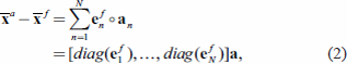
Following Lorenc (2003), we introduced the flow dependency of the forecast error by assuming that the analysis increment  belonged to the subspace spanned by the ensemble forecast perturbations. Hence, the analysis increment can be written with ensemble forecast perturbations
and their amplitudes an (Wang 2010) as follows:
where
diag ( ) is an operator that transforms a vector into a diagonal matrix and
a is a vector formed by concatenating
N vectors
an,
n = 1,
N.
As shown in Fig. 3, we employed ensemble forecasts within a box of horizontal grid points (reduced-grid box) neighboring the target point [hereafter referred to as the neighboring ensemble (NE)] to increase the ensemble sample size. We adopted 5 × 5 grids as a reduced-grid box, which was comparable to the CRM effective spatial resolution. The NE for the given ensemble member n within the M-point reduced-grid box can be written as  , where M is 25 in this study. We use m as the subscript denoting the point within the reduced-grid box. Further, we horizontally divided (xNE)fn,m into a large-scale portion (xL)fn and deviations (xd)fn,m and transformed them into a dual-scale NE (DuNE):
where

.
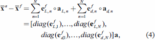
When we applied DuNE to EnVar, we reduced the dimension of the forecast perturbation subspace for the deviations. To this end, we first calculated the singular value decomposition (SVD) eigenmodes of the vertical cross covariance of the deviation forecast perturbations. Then, we approximated the ensemble forecast perturbations for the deviations using the first–Nth eigenvectors vn and eigenvalues λn. The analysis increment can be written with ensemble forecast perturbations for the large-scale portion and the deviation 
and their amplitudes aL, n, ad, n as follows:
where

denotes the ensemble mean of the largescale portion and
a is a vector obtained by concatenating vectors
aL, n,
n = 1,
N and
ad, n,
n = 1,
N.
By substituting Eq. (4) into Eq. (1), the cost function can be written in terms of a as follows:
where
A is the correlation matrix for
a expressed as a block diagonal matrix with correlation matrices for the large-scale portion and deviations
AL and
Ad. We iteratively minimized
Eq. (5) to achieve optimal analysis.
c. Estimation of the observation error covariance of MWI TBs
We used the method proposed by Desroziers et al. (2005) to estimate the observation error covariance R of MWI TBs. In this estimation, we neglected the off-diagonal terms of R to ensure simplicity.
First, we substituted the constant value (9.0 K2) into the diagonal terms of R as the first guess of the observational error variance. Next, we applied the following steps iteratively.
-
1) Execution of the DuNE EnVar to calculate the MWI TB innovation
 and the post-fit residuals
-
2) Estimation of R as the domain average of (df)(da)t.
We empirically performed the aforementioned iteration thrice for this estimation. The MWI TB bias correction has been described in Sections 3.2c and 3.3d.
d. Analysis for each ensemble member
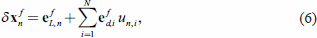
We applied the method proposed by Bishop et al. (2001) to calculate the analysis for each ensemble member.
First, we expressed the forecast increment for a member  in the DuNE forecast perturbation space (efL,n, efd,n).
where
un,i, denotes the
δxfn amplitude for the
ith SVD mode of the deviation. Then, we calculated the transform matrix from the forecast increments to the analysis increments in the DuNE forecast perturbation space
T as follows:
-
1) We obtained the observation perturbation matrix V and C = VtV for the DuNE forecast perturbations.
-
2) We derived T from the SVD eigenmatrix Γ and the eigenmodes U of C.
We calculated the analysis increment 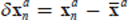 by multiplying T to Eq. (6).
Following Zhang et al. (2004), we inflated the analysis covariance by setting the analysis increment for each ensemble member as the weighted average of δxan and δxfn.
where we used the empirical weight
ω = 0.9.
3.2 Introduction of the non-Gaussian precipitation PDF
First, we evaluated the fits of the NE forecast perturbations for the target cases (Section 2.1) regarding the existing non-Gaussian PDF models and selected the best fitting PDF model. Then, we improved EnVar using the selected PDF model. Statistical fitting is not required between the precipitation observation and forecasts in this method.
a. Fits of the NE forecast perturbations to the
existing non-Gaussian PDF models
We selected the normal distribution (N), mixed normal distribution (MN), lognormal distribution (LN), and mixed lognormal distribution (MLN) as possible PDF models.
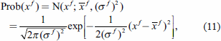
The N model assumed the PDF of the NE forecasts of a certain variable xf, i.e., Prob(xf), as follows:
where

and
σf are the mean and the standard deviation (STD) of
xf, respectively. We used the PR as
xf without any transformation.
In the MN model, the probability distribution of xf was assumed to be a mixture of Gaussian modes (regimes).
where
j is the superscript denoting the regime,
wf,j = Prob (
r = j) is the prior probability of regime
j, xf,j is a forecast belonging to regime

and
σf,j are the average and STD of
xf,j, respectively, and
jmax is the total number of regimes.
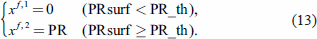
We adopted a two-regime model (jmax = 2) comprising a rain-free regime (r = 1) and a rainy regime (r = 2). While calculating the fit of PR to this model, we considered PR as zero when the surface precipitation rate (PRsurf) was weaker than the prescribed threshold (PR_th), following Kedem et al. (1990). We set PR_th to 0.3 mm h−1, which was comparable with the minimum detectable value of the GPM dual-frequency precipitation radar. Then, we can write xf,j as follows:
We considered the prior probability of each regime as the ratio of the NE number of the regime to the total NE number.
In the LN model, lnp = ln (PR + 1) was considered as xf to make the logarithm finite for PR ∼ 0. This model assumed a normal distribution of lnp and adopted Eq. (11) as the PDF of xf. The MLN model assumed two regimes of xf,j as follows:
Furthermore,
Eq. (12) was adopted as the PDF of
xf,j.
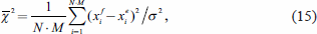
We adopted the  provided by Lien et al. (2016) to measure the fits of the NE forecast perturbations with the existing PDF models.
where
i is the rank of
xf for the given NE member and
xei is the value given by the PDF model
e for
i. xei can be written using the NE mean and STD of

, and the PDF model-normalized deviation for
i, F(
i), as follows:
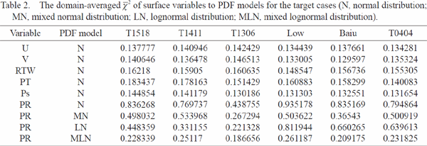
First, we verified the fits of the NE forecast perturbations of the surface variables to the N model for the target cases mentioned in Section 2.1. The  value of precipitation (0.44–0.94) was worse than those of the remaining variables (∼ 0.15), as presented in Table 2.
Next, we examined the fits of the NE forecast perturbations of surface precipitation to other PDF models for the same cases. The fits of the MLN models were considerably better than those of the remaining models, as presented in Table 2. The  value for the MLN model was similar to the value of other variables in case of the N model, whereas the
  values for the MN and LN models were more than double the values of other variables.
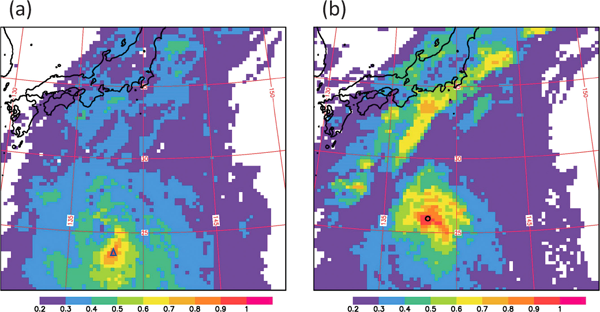
Figure 4 shows the distribution of  for the PDF models calculated from 14-h CRM ensemble forecasts (after DEC) for T1518. The
  value for the N model (Fig. 4a) was > 0.4 in majority of the precipitation areas and exceeded 1.0 around the typhoon center and the periphery of the front. The MN model (Fig. 4b) exhibited a better fit when compared with the N model in case of weak precipitation, particularly for the front periphery. The fit to the LN model (Fig. 4c) was considerably improved in the heavy-rain areas around the typhoon center and the front compared with the N model. The
  value for the MLN model (Fig. 4d) was < 0.3 and smaller than those of the remaining models for majority of the precipitation area.
b. Introduction of the MLN model for precipitation to EnVar
Based on the above results, we selected the mixed lognormal distribution as the precipitation PDF model. To introduce this model, we expanded EnVar to a type of Gaussian sum filter (Ristic et al. 2003) using two Gaussian PDF regimes, i.e., the rain-free and rainy regimes.
For this expansion, we classified the NE forecasts in a reduced-grid box into rain-free and rainy regimes using the threshold for surface precipitation (0.3 mm h−1). We set lnp as zero at all levels for the rain-free regime and transformed the classified NE forecasts into the DuNE for each regime (r = j), zf,j. When considering the MLN model, the PDF of the DuNE in the reduced-grid box can be expressed as a mixture of two Gaussian regimes:
where

and
Pf,j are the mean and the forecast error covariance of
zf,j respectively, and |
Pf,j| denotes the determinant of
Pf,j.
Aonashi et al. (2016) indicated that NE was not applicable to EnVar when the prior probability of each regime (the ratio of the NE number of the regime to the total NE) was < 0.1 due to the large sampling error. Accordingly, we set the prior probability of that regime as zero.
It should be noted that the rainy regime had the NE mean and the forecast error covariance of the precipitation variables larger than those calculated from the all-member ensemble. Figure 2d displays the rainy regime mean of the 14-h CRM ensemble forecasts (after DEC) for T1518. Compared with that in Fig. 2c, the precipitation increased around the typhoon center (Region A) and the front (Region B).
As the next step, we substituted the DuNE of each regime into EnVar to calculate the analysis of the regime mean  and the analysis error covariance of that regime Pa,j. The analysis of the all-member ensemble mean
  and the analysis error covariance Pa can be written as follows:
where
wa,j = Prob (
r = j | y
o) is the regime conditional probability for
j given the observation y
o (hereafter referred to as RCPO), which will be described in Section 3.2d.
c. Bias and normality of (TBo–TBc) of the regimes
Based on the study of Geer and Bauer (2011), we verified the bias and the normality of the difference of TBo–TBc calculated from the mean of the CRM forecasts of the rain-free and rainy regimes (rain-free mean TBc and rainy mean TBc, respectively). In this calculation, we selected grid points with a prior probability greater than 0.1. We excluded the points at which |TBo–TBc| was greater than thrice the ensemble spread of each regime. Hereafter, the points at which TBc is calculated for the rain-free (rainy) regime will be referred to as the calculated rain-free (rainy) areas. For comparison, we also computed TBc from the all-member ensemble mean of the CRM forecasts (after DEC) for the calculated rain-free and rainy areas (hereafter referred to as all-member mean TBc).
Figure 5a shows the joint PDF for TBo and the above TBcs for GMI TB18v at 14 UTC, September 7, 2015. The all-member mean TBc exhibited a significant (TBo–TBc) bias in the calculated rainy areas, which increased with TBo. The bias depended on the rain rate because TB18v is sensitive to rain emission over the ocean. In contrast, the rainy mean TBc exhibited a distribution close to 1:1 with respect to TBo. The (TBo–TBc) spreads were amplified in the calculated rainy areas, regardless of the regime classification.
Next, we checked the normality of the PDF of (TBo–TBc) standardized with the mean and STD of (TBo–TBc) for the calculated rain-free and rainy areas. The all-member mean TBc had a large separation from the normal distribution observed over the calculated rain-free areas, as shown in Fig. 5b. When compared with this, the normality was much better for the rain-free mean TBc.
These results indicate that the introduction of regime means into TBc calculation improved the bias and normality of (TBo–TBc). Therefore, we adopted the (TBo–TBc) averaged over the calculated rain-free and rainy areas as the TBo bias corrections for both regimes. However, we separately estimated the observation error covariance for each regime using the method described in Section 3.1c. Table 3 presents the observation error STDs of the GMI TBo with vertical polarization for the rain-free and the rainy regimes for 14 UTC, September 7, 2015. The observation error STDs had larger values for the rainy regime than the rain-free regime, reflecting the differences in the (TBo–TBc) spreads.
d. Conditional probability of the rain-free and rainy regimes
The RCPO of regime j, wa,j = Prob (r = j | yo), can be estimated from the prior probability and the model-conditioned likelihood function (MCLF), Prob (yo | r = j), using Bayes' theorem.
To estimate the RCPO given GMI TBs at the five frequencies with vertical polarization as the observation, we employed the prior probability of Section 3.2b. Then, we approximated the MCLF for each regime by assuming normal distribution of the differences between the bias-corrected TBo and the TBc calculated from DuNE,
zf,jn,m.
where
Mjn is the total number of points for regime
j within the reduced-grid box for ensemble member
n,

is the mean of
df,jn,m that is assumed as a zero vector because the TBo bias was corrected, and
Sj is the covariance matrix of the (TBo–TBc) estimated from the DuNE of each regime.
Figure 6 shows the RCPO of each regime for the 14-h CRM ensemble forecasts (after DEC) starting at 00 UTC, September 7, 2015. The RCPO was close to one for either regime at many points due to the high sensitivity of the MWI TBs to precipitation. However, both the regimes exhibited an RCPO of zero for the observed rainy areas south of the front and around the typhoon, where the MCLF of the rain-free regime and the prior probability of the rainy regime were zero. An RCPO of zero was also found for the observed heavy-rain areas near the typhoon (Region E), where the CRM ensemble forecasted only weak precipitation.
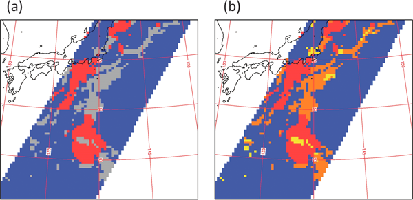
Figure 7 a shows the regimes with maximum RCPO at 14 UTC, September 7, 2015. There were many points at which no regimes had a positive RCPO because of the precipitation displacement error or a false heavy precipitation forecast. In other words, no regimes corresponded to TBo.
3.3 New method for correcting the precipitation displacement
Equation (18) indicates that the EnVar analysis results in a zero value for grid points at which both regimes have a zero RCPO. To avoid this, we developed a new precipitation displacement correction method using PDF pseudo-regimes.
a. PDF pseudo-regimes
The results in Section 3.2d indicate that an RCPO of zero was found for both the regimes at the following points:
-
1) Rain-free areas in the real atmosphere, where the ensemble forecasts had no rain-free regime.
-
2) Rainy areas in the real atmosphere, where the ensemble forecasts had no rainy regime.
-
3) Heavy-rain areas in the real atmosphere, where the ensemble forecasts gave only weak precipitation.
We introduced the pseudo rain-free, rainy, and heavy-rain regimes to address these points. We selected the regional average of the PDFs of the rain-free, rainy, and heavy-rain regimes from many alternatives for approximating the PDF pseudo-regimes owing to its simplicity. We defined the heavy-rain regime as NE forecasts with a surface precipitation greater than 3 mm h−1.
We employed regional averages only for lnp, w, and RTW for the large-scale portion of the PDFs. Further, we used the all-member ensemble PDFs at the target point for the remaining variables to avoid the smoothing of synoptic-scale disturbances.
b. Horizontal scales of PDF averaging
We need to set the range of PDF averaging for pseudo-regimes. To this end, we evaluated the horizontal scales of the similarity of their ensemble forecast perturbations. We specifically verified the similarity of the vertical correlation of the ensemble forecast perturbations in case of the rain-free, weak-rain, and heavy-rain points and their surrounding areas for T1518. As a similarity index, we employed the commonly used Dice coefficient (DC) defined for the two vectors a and b as follows:
where the dot indicates the inner product of the vectors and
a and
b are the vectors that represent the vertical correlation of the ensemble perturbations at the target points.
Figure 8 shows the DCs for a rain-free point (△ in Fig. 8a) and a heavy-rain point (○ in Fig. 8b) for 14-h CRM ensemble forecasts (after DEC) starting at 00 UTC, September 7, 2015. The similarity range (DC > 0.6) of the ensemble forecast perturbations was local (∼ 250 km) for rain-free points. The same similarity range was found for weak-rain points (figure not shown). In contrast, the ensemble forecast perturbations for heavy rain were similar to each other over a much wider range.
Based on these results, we set the range of PDF averaging to 250 km within the target points for the pseudo-rain-free and rainy regimes. We did not define the PDF of the pseudo-rain-free (rainy) regime when we had no points with the rain-free (rainy) regime in the PDF averaging range. We used the PDF averaged over the whole domain of the CRM for the pseudo-heavy-rain regime.
c. Introduction of PDF pseudo-regimes to EnVar
We added three pseudo-regimes to Eq. (17) and reset jmax as 5. We also prescribed the prior probabilities of the pseudo-regimes as 0.01, which was negligible compared with those of the rain-free and rainy regimes (> 0.1). Then, the ensemble mean analysis and the analysis error covariance calculation were conducted regarding those in the five regimes and their conditional probabilities based on Eq. (18).
Figure 7b illustrates the regimes, including the pseudo-regimes, with the maximum RCPO for 14 UTC, September 7, 2015. The RCPO was close to one for either regime at most points due to the high sensitivity of MWI TBs to precipitation. The pseudo-rainy regime occupied majority of the points at which no regimes corresponded to TBo in Fig. 7a (pseudo-rainy areas). The pseudo-heavy-rain regime was most likely around the typhoon center (pseudo-heavy-rain areas).
d. Bias and normality of (TBo—TBc) of the pseudo-regimes
We verified the bias and normality of the difference between TBo and TBc calculated from the means of the CRM forecasts of the pseudo-regimes with the maximum RCPO (pseudo-mean TBc). We selected grid points at which both the rain-free and rainy regimes had an RCPO of zero. These points will be referred to as pseudo-areas.
Figure 5c shows the joint PDF for TBo and the pseudo-mean TBc, the all-member mean TBc for the pseudo-areas, and the calculated rain-free areas for GMI TB18v at 14 UTC, September 7, 2015. The all-member mean TBc had no sensitivity to TBo for the pseudo-areas and had values identical to those of the calculated rain-free areas. In contrast, the pseudo-mean TBc had a distribution close to 1:1 regarding TBo, which is similar to the rainy mean TBc in Fig. 5a. The spreads of the pseudo-mean TBc from TBo were comparable with those of the rainy mean TBc.
Next, we verified the normality of the PDF of (TBo–TBc) standardized with the mean and STD of (TBo–TBc) for pseudo-areas. The all-member mean TBc exhibited a large separation from the normal distribution over the pseudo-areas, as shown in Fig. 5d. In particular, the mode of distribution was found near −1. In comparison, the normality was much better for the pseudo-mean TBc.
Based on these results, we adopted the mean of (TBo–TBc) and the observation error covariance over rainy areas as the TBo bias correction values and the observation error covariance for the pseudo-regimes, respectively.
3.4 Streamlining EnVar
The EnVar in Section 3.3 c incurred a large computational cost because it minimized the cost functions for five regimes, although the ensemble mean analysis barely reflected the EnVar analyses of the regimes, except for that with the maximum RCPO. This is because the maximum RCPO was close to one for majority of the points due to the high sensitivity of MWI TBs to precipitation.
We streamlined EnVar by introducing a composite of DuNE based on the most likely regime for each grid point. The usage of the DuNE composite is similar to that in the method proposed by Montmerle and Berre (2010), wherein the covariance of the forecast error was expressed as a combination of the values associated with the rain-free and rainy regions. The mean of the ensemble forecasts  and the forecast perturbation covariance Pf can be written as follows:
where
wf,jst is the weight, which is one for the most likely regime and zero for the remaining regimes.
We added the following preparation procedures to EnVar to achieve approximation.
-
1) Calculate TBc from the mean of DuNE of the regimes.
-
2) Estimate the RCPO of the regimes from TBo and TBc.
-
3) Calculate
 and Pf from the DuNE of the most likely regime for each grid point.
The usage of  and Pf enabled us to achieve ensemble mean analysis by minimizing the single cost function.
4. Assimilation and forecast experiments for T1518
We performed experiments that assimilated each observation at a certain time (hereafter referred to as single-time observation experiments) using the same ensemble forecasts to examine the impacts of the assimilation methods on analysis and forecast. We also verified the impact of a forecast analysis cycle when compared with a single-time observation experiment.
4.1 Single-time observation experiments
a. Description of the experiments
We performed experiments that assimilated all-sky GMI TBs and conventional observation data at 14 UTC, September 7, 2015, using CRM ensemble forecasts after DEC (started at 00 UTC, September 7, 2015). We also executed a CRM forecast using the resultant analysis of the all-member ensemble mean (hereafter referred to as analysis for simplicity) as the initial data.
First, we performed the following experiments to determine the performance of the EnVar employed in this study:
-
1) FG: an experiment without assimilation. The analysis resulted in a value equal to the all-member mean of the CRM ensemble forecasts after DEC for 14 UTC, September 7, 2015, as the initial value.
-
2) CN: an assimilation using the EnVar employed in this study wherein the mixed lognormal PDF and a new displacement correction method were used.
Next, we verified the impacts of introducing the mixed lognormal PDF and a new displacement correction method using PDF pseudo-regimes with the following experiments:
-
1) GD: assimilation with the conventional EnVar by adopting a single normal PDF regime for precipitation. In this experiment, we separately estimated the TB bias and the observation error STD from the all-member mean of (TBo–TBc) over the calculated rain-free areas and other areas.
-
2) MLD: assimilation with an experimental EnVar that used only the mixed lognormal PDF and that did not use the new displacement correction method.
In addition, we investigated the forecast impacts of the analysis increments of the water substances and other variables through the following forecast experiments:
-
1) NW: the same as CN but with zero analysis increments for water substances and w.
-
2) ND: the same as CN but with zero analysis increments for u, v, PT, and Ps.
Further, we examined the contribution of DEC to assimilation using the EnVar employed in this study and the CRM forecasts. Therefore, we performed an experiment skipping DEC (SD), which was similar to CN, but using the CRM ensemble forecasts without DEC (started at 00 UTC, September 7, 2015).
b. Impacts on analysis
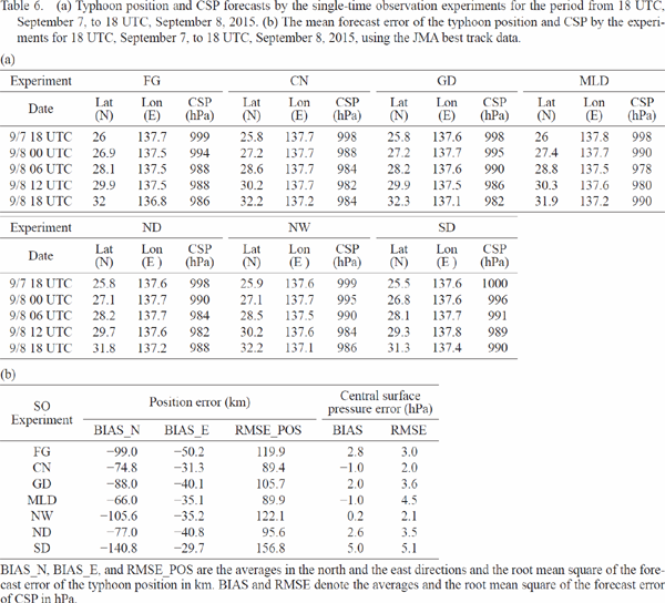
First, we describe the increments of CN analysis minus the all-member mean of the CRM ensemble forecasts, which was equal to that of FG analysis. Figure 9 shows the CN analysis increments and FG analysis for the surface precipitation, w at a height of 5000 m, RTW at a height of 1460 m, and pressure and horizontal winds at the surface.
CN resulted in increased surface precipitation around the typhoon, particularly to the north of the typhoon center (Region F), as indicated in Fig. 9a. CN also induced precipitation in the pseudo-rainy areas to the south of the front (Region G) and east of the typhoon, where FG missed precipitation.
In Fig. 9b, CN increased w in the aforementioned areas with positive precipitation increments. However, in the southern part of the front, CN yielded negative W increments (Region H) in positive precipitation increment areas because CN employed the mean of DuNE of the rainy regime as the EnVar first guess for this area. When we derived the analysis increments from the rainy regime mean, CN had negative increments for both the surface precipitation and w (figures not shown).
CN moistened the pseudo-rainy areas, whereas the humidity increments were small for the heavy-rain areas, as indicated in Fig. 9c. Moreover, CN moved the moist areas associated with the typhoon southeast-ward by giving positive increments toward the east (Region I) and negative increments toward the north and west of its center (Region J).
EnVar realized analysis increments of the pressure and winds around the typhoon, as shown in Fig. 9d; here, these variables exhibited a significant ensemble forecast perturbation correlation with precipitation. CN moved the low-pressure area of the typhoon eastward by giving negative increments to the east (Region K) and positive increments to the west of its center (Region L). The surface horizontal wind increments corresponded to this dipole pattern of the increments in Ps.
Next, we compared the analyses of single-time observation experiments to examine the impact of the analysis methods used in this study. Table 4a presents the quantitative validation results of the experimental precipitation analyses using GSMaP retrieval for 14 UTC, September 7, 2015. We used the reduced-grid box (25 × 25 km) averages of the data for validation. AVE indicates the average of the experimental precipitation data in mm h−1. The BIAS and RMSE are the average and root mean square error, respectively, of the experimental precipitation data minus the GSMaP retrieval in mm h−1. TSh and TSw denote the threat scores for heavy (threshold: 10 mm h−1) and whole (threshold: 0.1 mm h−1) rain events, respectively. Figure 10a illustrates the GSMaP surface precipitation for 14 UTC, September 7, 2015. Figures 10b–f illustrate the analyses for precipitation, pressure, and horizontal winds at the surface given by FG, CN, GD, MLD, and SD.
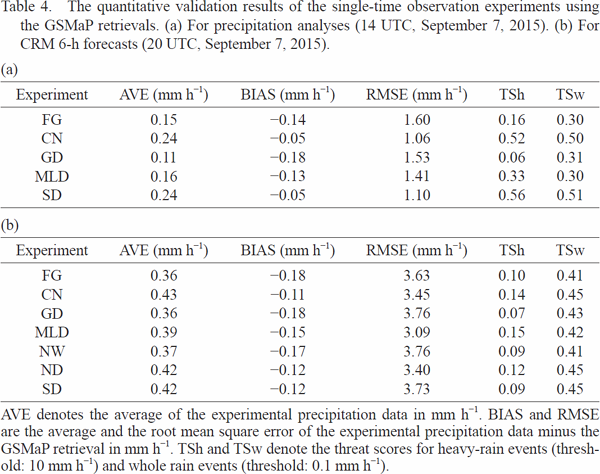
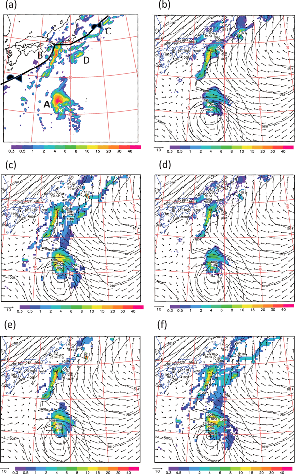
Table 4a and Fig. 10b show that FG underestimated the surface precipitation compared with GSMaP (BIAS = −0.14 mm h−1). CN reduced the underestimation (BIAS = −0.05 mm h−1) and RMSE (1.06 mm h−1) when compared with FG. It also resulted in considerably higher threat scores (TSh = 0.52 and TSw = 0.50) than FG (TSh = 0.16 and TSw = 0.32), indicating that the EnVar employed in this study generally improved the precipitation analysis. Compared with the GSMaP retrieval, CN (Fig. 10c) was successful in reproducing most of the GSMaP rainy areas by inducing precipitation in the pseudo-rainy areas. It also achieved a precipitation analysis similar to that obtained by GSMaP retrievals for Regions A and B. These were reflected in the high TSh and TSw values.
The BIAS (−0.18 mm h−1) and TSh (0.06) of GD were worse than those of FG because GD missed the precipitation in the pseudo-rainy areas and yielded a much weaker precipitation analysis than GSMaP for heavy-rain areas (Fig. 10d). In contrast, the TSh (0.33) of MLD was an intermediate value between those of FG and CN, whereas its TSw (0.30) was close to that of FG. It resulted in a precipitation analysis similar to the GSMaP retrieval for most of the heavy-rain areas (Fig. 10e). However, only weak precipitation was analyzed for the pseudo-heavy-rain area within Region A, resulting in the intermediate value of TSh. MLD also missed the precipitation in the pseudo-rainy areas, resulting in a low TSw.
SD had high threat scores (TSh = 0.56 and TSw = 0.51) similar to those of CN. Figure 10f depicts that SD was successful in achieving a precipitation analysis similar to the GSMaP retrieval while the typhoon center was displaced southward from that given by CN.
The results indicate that the introduction of the mixed lognormal PDF strengthened the precipitation analysis, thereby achieving data similar to the GSMaP retrievals for heavy-rain areas. We also tested EnVar by assuming the mixed normal PDF of precipitation. The assimilation experiment performed using this scheme resulted in an analysis similar to MLD (figure not shown). Based on this result, using the PDF of the rainy regime and the resultant TBo bias reduction contributed to the retrieval of the heavy precipitation.
Furthermore, using the PDF pseudo-regimes considerably reduced the precipitation displacement error of the analysis and contributed to the heavy-rain analysis in the pseudo-heavy-rain areas. The comparison between CN and MLD indicated that a large part of the humidity analysis increments can be attributed to the introduction of the pseudo-rainy regime (figure not shown). The SD results also indicated that using the PDF pseudo-regimes without DEC can correct the precipitation displacement error of the analysis for the target case.
c. Impacts on CRM forecasts
First, we describe the impacts of the assimilation methods of this study on the 6-h CRM forecasts. Table 4b presents the quantitative validation results of the 6-h precipitation forecasts of the experiments using GSMaP retrieval for 20 UTC, September 7, 2015. Figure 11a illustrates the GSMaP surface precipitation for 20 UTC, September 7, 2015. Figures 11b–h display the 6-h CRM forecasts of the experiments for precipitation, pressure, and horizontal winds at the surface.
As shown in Fig. 11a, GSMaP indicated heavy rain from the west to the north of the typhoon center (Region Ma). Heavy-rain areas were also retrieved for the front from the south of Kanto to the ocean east of Tohoku (Region N).
Then, we compared FG and CN with GSMaP retrieval to see the impacts of the analysis methods of this study on the forecast. FG underestimated the surface precipitation when compared with GSMaP (BIAS = −0.18 mm h−1), as presented in Table 4b. Furthermore, FG displaced the typhoon position southward of the best track, as illustrated in Fig. 11b. FG also forecasted heavy rain from the east to the north of the typhoon center (Region Mb), which was considerably weaker than GSMaP retrieval. Moreover, FG exhibited a northwest precipitation displacement error with respect to Region N. In contrast, CN reduced the underestimation (BIAS = −0.11 mm h−1) and RMSE (3.45 mm h−1) when compared with FG (Table 4b); further, it yielded higher threat scores (TSh = 0.14 and TSw = 0.45) than FG (TSh = 0.10 and TSw = 0.41). Thus, the EnVar employed in this study improved the 6-h precipitation forecast. CN provided a better typhoon position forecast than FG by moving the typhoon center northward, as illustrated in Fig. 11c. CN had a higher TSh than FG by strengthening the precipitation around the typhoon (Region Mc). However, the TSh for the CN forecast worsened when compared with that for the analysis because heavy-rain areas were displaced around the typhoon. (CN reduced the precipitation displacement error regarding Region N, resulting in a higher TSw than FG.
We verified GD and MLD for the forecast contribution of both assimilation methods. Table 4b indicates that GD had the worst TSh among the experiments because it forecasted weaker precipitation than FG around the typhoon (Fig. 11d). In contrast, the TSh (0.15) of MLD was comparable with that of CN, whereas its TSw (0.42) was close to that of FG. Figure 11e illustrates that MLD was similar to CN around the typhoon, resulting in a high TSh. MLD was similar to FG for Region N, which was reflected in the low TSw. These results indicate that the introduction of the mixed lognormal PDF contributed to the improvement of heavy-rain forecast around the typhoon and that the use of PDF pseudo-regimes reduced the precipitation forecast displacement error around the front.
We also compared NW and ND to see the forecast impacts of CN analysis increments regarding water substances and other variables. Table 4b indicates that NW (ND) provided the same value of TSw as FG (CN), whereas the TSh values of both of them were lower than that of CN. Figures 11f and g show that NW and ND resulted in intermediate values regarding those of CN and FG for heavy-rain forecasts around the typhoon. NW and ND were similar to FG and CN, respectively, for the precipitation forecast around the front. Thus, both the water substances and other variables improved the forecast of heavy rain around the typhoon. Furthermore, water substances considerably influenced the reduction of the precipitation forecast displacement error around the front.
We verified the impacts of DEC on the 6-h CRM forecast by comparing CN and SD. SD resulted in a lower TSh (0.09) than CN (0.14), as presented in Table 4b. As shown in Figs. 11c and 11h, this can be mainly attributed to the fact that SD forecasted a weaker precipitation around the typhoon center when compared with CN. CN forecasted areas with a precipitation heavier than 20 mm h−1 toward the north of the typhoon center, and SD forecasted heavy precipitation ∼ 40 km north of the typhoon center. The results suggest that the correction of the typhoon center position with DEC improved not only the typhoon position forecasts but also the precipitation forecasts around the typhoon.
We also compared the CRM forecasts of the experiments over a longer period. Table 5 presents the quantitative validation results of CRM up to-18 h forecasts for the 3-h-averaged precipitation given by FG and CN using GSMaP retrieval for 14 UTC 7–05 UTC, September 8, 2015. This indicates that the EnVar employed in this study improved the BIAS and the threat scores of the CRM precipitation forecasts for 12 h.

In contrast, the experiments retained distinct forecast differences for > 24 h regarding the position and the CSP of the typhoon with a life span of a few days (Table 6a. Fig. 12). We calculated the period–mean forecast error of the typhoon position and CSP of the experiments to evaluate the impacts of the EnVar employed in this study on the typhoon forecasts (Table 6b). For this calculation, we used the JMA best track data as the truth data. BIAS_N, BIAS_E, and RMSE_POS are the averages in the north and east directions and the root mean square of the forecast error of the typhoon position in kilometers, respectively. BIAS and RMSE denote the averages and the root mean square of the forecast error of CSP in hPa, respectively.

A comparison of CN and FG with the best track showed that CN yielded better typhoon position forecasts (RMSE_POS = 89.4 km) than FG (RMSE_POS = 119.9 km) based on the forecast of the typhoon locations north to the northeast of FG. CN also provided better typhoon intensity forecasts (BIAS = −1.0 hPa and RMSE = 2.0 hPa) than FG (BIAS = 2.8 hPa and RMSE = 3.0 hPa) by lowering the CSP. This means that the EnVar employed in this study improved the typhoon forecasts for > 24 h. By examining the evolution of the CRM forecasts of the experiments, we found that CSP deepening occurred after the formation of heavy-rain areas near the typhoon center (figure not shown).
GD yielded typhoon forecasts (RMSE_POS = 105.7 km and RMSE = 3.6 hPa) similar to those of FG. MLD showed northward movement of the typhoon (BIAS_N = −66.0 km) faster than CN, and its RMSE_POS (89.9 km) was comparable with that of CN. MLD also had the same mean forecast error of CSP (BIAS = −1.0 hPa) as CN; however, its RMSE (4.5 hPa) was worse due to the large temporal variation of CSP. The mixed lognormal PDF considerably affected the typhoon forecasts. The PDF pseudo-regimes also had significant impacts.
We compared NW and ND with CN and found that ND resulted in typhoon position forecasts (RMSE_POS = 95.6 km) close to those of CN. The forecast error of NW was comparable with that of CN for the typhoon CSP (BIAS = 0.2 hPa and RMSE = 2.1 hPa). These interesting results indicate that the changes in water substance mainly affected the typhoon position forecasts, whereas the increments of other variables had impacts on the typhoon intensity forecasts.
SD forecasted the slowest northward movement (BIAS_N = −140.8 km) and the shallowest CSP (BIAS = 5.0 hPa) of the typhoon. The underestimation of CSP deepening can be mainly attributed to the displacement of heavy-rain areas from the typhoon center in SD forecast (Fig. 11h). This suggests that DEC improved the typhoon intensity forecast by reflecting the observed relative location between the typhoon center and the heavy-rain areas to the analysis.
4.2 Comparison between the forecast analysis cycle and single-time observation assimilation
a. Description of the experiments
We examined how the assimilation of MWI TBs with a forecast analysis cycle improved CRM forecasts compared with a single-time observation assimilation. Hence, we performed the following two experiments with the EnVar employed in this study.
-
1) SO: a single-time observation assimilation incorporating the all-sky AMSR2 TBs and conventional data for 17 UTC, September 8, 2015, using the CRM ensemble forecasts started at 00 UTC, September 8.
-
2) FA: a forecast analysis cycle, which assimilated the all-sky MWI TBs and conventional data for 14 UTC, 7 (GMI), 07 UTC, 8 (SSMIS), and 17 UTC, 8 (AMSR2), September 2015, using the CRM ensemble forecasts started at 00 UTC, September 7.
First, we describe the observed precipitation features in the vicinity of Japan at 17 UTC, September 8, 2015, using JHP (Fig. 13a) and AMSR2 TB89v (Fig. 13b). At this time, T1518 moved northward over the ocean south of Tokai, and its surrounding precipitation covered a wide range from western to northern Japan. Heavy rain (PR > 10 mm h−1) was observed over the ocean north of the typhoon center (Region O). Other heavy-rain areas were located in western Kanto (Region P) and were considered as orographic shallow rain due to the small depression of AMSR2 TB89v. In addition, there was a narrow rain band, including heavy rain from the Sea of Japan to the ocean south of Shikoku.
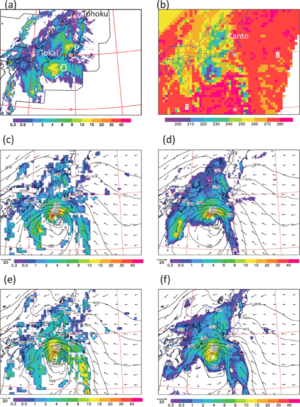
We also compared the analyses of SO and FA with the observation. Table 7a presents the quantitative validation results of the experimental precipitation analyses using JHP for 17 UTC, September 8, 2015. This indicates that SO underestimated the surface precipitation compared with JHP (BIAS = −0.19 mm h−1) and that FA reduced the underestimation (BIAS = −0.05 mm h−1). FA also resulted in a considerably higher TSh (0.24) than SO (0.17). As shown in Figs. 13c and 13e, SO overestimated (underestimated) the southern (northern) part of Region O, whereas FA gave a precipitation pattern close to that of JHP. This was reflected in the better TSh of FA when compared with that of SO. This difference was mainly caused by SO having a southward displacement error in the EnVar first guess, whereas the first guess of FA yielded a realistic precipitation for Region O. Both SO and FA failed to retrieve the heavy rain regarding Region P probably because the CRM could not reproduce this shallow orographic rain. This failure made the TSh of the FA analysis (0.24) significantly lower than that of CN analysis (0.52).
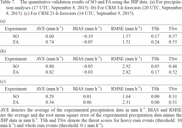
First, we compared the 3-h CRM forecasts of the experiments with JHP. Table 7b presents the quantitative validation results of the 3-h precipitation forecasts of the experiments using JHP for 20 UTC, September 8, 2015. Figure 14a displays the JHP for this time. Figures 14b and 14c show the 3-h CRM forecasts for the precipitation, pressure, and horizontal winds at the surface given by SO and FA, respectively.
Figure 14a shows that T1518 rapidly moved northward, and the heavy-rain areas north of its center (Region Q) were over the coastal regions from Tokai to Kanto at this time.
FA resulted in higher threat scores (TSh = 0.17 and TSw = 0.52) than SO (TSh = 0.05 and TSw = 0.48), as indicated in Table 7b. SO displaced Region Q by ∼ 100 km and FA agreed well with JHP about the heavy-rain location, as shown in Figs. 14b and 14c. These differences resulted in improvements in the threat scores of FA when compared with those of SO. FA also resulted in a better typhoon position forecast compared with SO by moving the typhoon center northward. This resulted in a conclusion similar to that in Section 4.1c, wherein a better analysis around the typhoon improved the precipitation and position forecasts of the typhoon.
Next, we describe the CRM forecasts of the experiments after 12 h. Table 7c presents the quantitative validation results of the 21-h precipitation forecasts of the experiments using JHP for 14 UTC, September 9, 2015. Figure 15a displays the JHP for this time. Figures 15b and 15c show the 21-h CRM forecasts for the precipitation, pressure, and horizontal winds at the surface given by SO and FA, respectively.
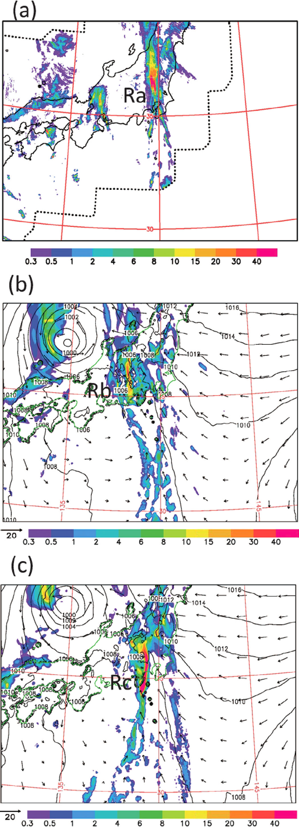
JHP showed that a heavy-rain band in the north–south direction stagnated at approximately 139–140°E after 05 UTC, September 9 (Region Ra). SO indicated a rain band at approximately 138°E at 05 UTC, September 9 (12-h forecast), which was not maintained subsequently. At 14 UTC, September 9 (21-h forecast), SO had a few weak-rain bands at approximately 137–138°E (Region Rb). FA indicated a rain band at approximately 138°E at 05 UTC, September 9, which was strengthened and stagnated around 138.5°E (Region Rc) until 23 UTC, September 10 (30-h forecast). However, even FA resulted in a TSh value of zero for the 21-h forecast because it still displaced the heavy-rain band by ∼ 100 km (Table 7c).
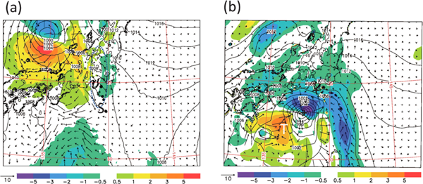
We estimated the forecast deviations, FA–SO, for various variables to find the reason for these differences in the forecasted rain band features. Figure 16a illustrates that lower tropospheric winds exhibited west-to-northwest deviations around the rain band (Region S). These wind deviations strengthened the precipitation and pushed the rain band eastward.
These deviations were collocated with the boundary of the positive pressure deviation area south of the typhoon. We checked the evolution of forecast deviations to find that the positive pressure deviations seemed to originate from the west and southwest of the typhoon at the initial time (Region T). Hence, the analysis of the dynamic variables around the typhoon may have contributed to an improved forecast for the rain band.
5. Summary and discussion
5.1 Summary
In this study, we considered the remaining issues of precipitation assimilation, the non-Gaussian PDF, and the displacement error of precipitation for better assimilation of the all-sky MWI TBs into a CRM.
We evaluated the fits of the precipitation forecast perturbations of various disturbance cases to the existing non-Gaussian PDF models with the chi-square value presented by Lien et al. (2016). Based on the obtained results, we decided to use the mixed log-normal distribution as the precipitation PDF model and introduced rain-free and rainy PDF regimes to the EnVar employed in this study. We also developed a new precipitation displacement correction method, which introduced the pseudo-rain-free, rainy, and heavy-rain regimes and approximated their PDFs as the regional average of the PDFs around the target point. The aforementioned methods improved the bias and normality of the TB differences between the observation and the first guess in rainy areas.
The experimental results for T1518 showed that the EnVar employed in this study resulted in precipitation analyses more similar to the GSMaP retrievals than the conventional EnVar using a single normal PDF regime for precipitation. Introducing the mixed log-normal PDF strengthened the precipitation analysis for the heavy-rain areas around the typhoon and the front. Using the PDF pseudo-regimes considerably reduced the precipitation displacement error of the analysis. The EnVar employed in this study also improved the CRM forecasts for the precipitation distribution up to 12 h and the typhoon position and CSP for > 24 h. The forecast analysis cycle of the EnVar improved the CRM forecasts for heavy rain around the typhoon center up to 6 h and the heavy-rain band associated with the typhoon for > 24 h compared to the EnVar wherein a single-time TB observation was incorporated.
5.2 Discussion
First, we discuss our approach to the non-Gaussian nature of precipitation. Previous studies, such as those conducted by Lien et al. (2016), focused on transforming precipitation into normally distributed control variables. The present study is characterized by the introduction of multiple PDF regimes for precipitation into EnVar by assuming a mixed lognormal distribution of precipitation.
This method improved the heavy-rain analysis compared to the conventional method by assuming normal precipitation distribution. This improvement can be mainly attributed to the usage of the ensemble mean and the forecast error covariance in case of the rainy regime. This made the mean and STD of precipitation of the EnVar employed in this study higher than those of the conventional method. Further, the (TBo–TBc) bias in rainy areas was reduced, as shown in Section 3.2.
Next, we discuss the features of the new displacement correction method presented in this study. In addition to the large-scale DEC presented in our previous study (Aonashi and Eito 2011), we introduced PDF pseudo-regimes for the rain-free, rainy, and heavy-rain regimes to EnVar. This method provided EnVar with PDF regimes corresponding to TBo and considerably reduced the precipitation displacement error of the analysis. For simplicity, we approximated the PDFs of the pseudo-regimes as the regional average of the PDFs around the target point. In the future, we aim to test other alternatives for pseudo-regime PDFs to evaluate their advantages and disadvantages.
In addition, we found a very interesting result that the ensemble forecast perturbations for heavy rain were similar over a wide range for T1518 (Fig. 8). This was convenient for the EnVar because areas with heavy rain were very confined in the CRM ensemble forecasts. However, to generalize this result, we must study many cases, including the TRMM and GPM observations.
Next, we discuss the impact durations of the precipitation assimilation of the forecasts. Many previous studies, including that of Tsuyuki and Miyoshi (2007), reported impact durations of up to 24 h, whereas Lien et al. (2013) reported a much longer duration of ∼ 5 days. The results of this study indicated that the impact durations were ∼ 12 h for precipitation forecasts and > 24 h for typhoon forecasts.
The long impact duration can be mainly attributed to the EnVar analysis increments that changed the position and intensity forecasts of the typhoon. The forecast impacts remained for a long period because EnVar changed the evolution of active disturbance with a lifespan of a few days.
Finally, we discuss the improvement in typhoon forecasts by all-sky MWI TB assimilation. We calculated the period–mean forecast error associated with the typhoon position and CSP using JMA best track data to evaluate the impacts of EnVar on the typhoon forecasts. Assimilation with the EnVar employed in this study improved the typhoon position and intensity forecasts for > 24 h. Furthermore, DEC contributed to the typhoon position and intensity forecasts. However, statistical verification must be conducted for various typhoons to generalize these results.
Interesting results were obtained from this study. The analysis increments of water substances mainly affected the typhoon position forecasts, whereas those of the remaining variables affected the typhoon intensity forecasts (Table 6b). The forecast analysis cycle improved the forecasts for the heavy-rain band associated with the typhoon. In the future, we aim to investigate these mechanisms.
Acknowledgments
This research is supported in part by Japan Aerospace Exploration Agency under the GPM research grant and Global Change Observation Mission-Water 1 research grant, and by Japan Society of the Promotion of Science Grands-in-Aid for Scientific Research (KAKENHI) grant number 15K05294.
References
- Aonashi, K., and H. Eito, 2011: Displaced ensemble variational assimilation method to incorporate microwave imager brightness temperatures into a cloud-resolving model. J. Meteor. Soc. Japan, 89, 175-194.
- Aonashi, K., K. Okamoto, T. Tashima, T. Kubota, and K. Ito, 2016: Sampling error damping method for a cloud-resolving model using a dual-scale neighboring ensemble approach. Mon. Wea. Rev., 144, 4751-4770.
- Bauer, P., A. J. Geer, P. Lopez, and D. Salmond, 2010: Direct 4D-Var assimilation of all-sky radiances. Part I: Implementation. Quart. J. Roy. Meteor. Soc., 136, 1868-1885.
- Bishop, C. H., B. J. Etherton, and S. J. Majumdar, 2001: Adaptive sampling with the ensemble transform Kalman filter. Part I: Theoretical aspects. Mon. Wea. Rev., 129, 420-436.
- Chambon, P., S. Q. Zhang, A. Y. Hou, M. Zupanski, and S. Cheung, 2014: Assessing the impact of pre-GPM microwave precipitation observations in the Goddard WRF ensemble data assimilation system. Quart. J. Roy. Meteor. Soc., 140, 1219-1235.
- Desroziers, G., L. Berre, B. Chapnik, and P. Poli, 2005: Diagnosis of observation, background and analysis-error statistics in observation space. Quart. J. Roy. Meteor. Soc., 131, 3385-3396.
- Draper, D. W., D. A. Newell, F. J. Wentz, S. Krimchansky, and G. M. Skofronick-Jackson, 2015: The Global Precipitation Measurement (GPM) microwave imager (GMI): Instrument overview and early on-orbit performance. IEEE J. Sel. Top. Appl. Earth Obs. Remote Sens., 8, 3452-3462.
- Errico, R. M., P. Bauer, and J.-F. Mahfouf, 2007: Issues regarding the assimilation of cloud and precipitation data. J. Atmos. Sci., 64, 3785-3798.
- Geer, A. J., and P. Bauer, 2011: Observation errors in all-sky data assimilation. Quart. J. Roy. Meteor. Soc., 137, 2024-2037.
- Geer, A. J., F. Baordo, N. Bormann, P. Chambon, S. J. English, M. Kazumori, H. Lawrence, P. Lean, K. Lonitz, and C. Lupu, 2017: The growing impact of satellite observations sensitive to humidity, cloud and precipitation. Quart. J. Roy. Meteor. Soc., 143, 3189-3206.
- Hoffman, R. N., and C. Grassotti, 1996: A technique for assimilating SSM/I observations of marine atmospheric storms: Tests with ECMWF analyses. J. Appl. Meteor., 35, 1177-1188.
- Ide, K., P. Courtier, M. Ghil, and A. C. Lorenc, 1997: Unified notation for data assimilation: Operational, sequential and variational. J. Meteor. Soc. Japan, 75, 181-189.
- Ikawa, M., and K. Saito, 1991: Description of a nonhydrostatic model developed at the Forecast Research Department of the MRI. Technical Reports of the Meteorological Research Institute No. 28, 245 pp.
- Imaoka, K., M. Kachi, M. Kasahara, N. Ito, K. Nakagawa, and T. Oki, 2010: Instrument performance and calibration of AMSR-E and AMSR2. Int. Arch. Photogramm. Remote Sens. Spat. Inf. Sci., 38, 13-16.
- Kedem, B., L. S. Chiu, and G. R. North, 1990: Estimation of mean rain rate: Application to satellite observations. J. Geophys. Res., 95, 1965-1972.
- Kubota, T., K. Aonashi, T. Ushio, S. Shige, Y. N. Takayabu, M. Kachi, Y Arai, T. Tashima, T. Masaki, N. Kawamoto, T. Mega, M. K. Yamamoto, A. Hamada, M. Yamaji, G. Liu, and R. Oki, 2020: Global Satellite Mapping of Precipitation (GSMaP) products in the GPM era. Satellite Precipitation Measurement. Levizzani, V, C. Kidd, D. Kirschbaum, C. Kummerow, K. Nakamura, and F. Turk (eds.), Advances in Global Change Research, 67, Springer, 355-373.
- Kunkee, D. B., G. A. Poe, D. J. Boucher, S. D. Swadley, Y. Hong, J. E. Wessel, and E. A. Uliana, 2008: Design and evaluation of the first Special Sensor Microwave Imager/Sounder. IEEE Trans. Geosci. Remote Sens., 46, 863-883.
- Lien, G.-Y, E. Kalnay, and T. Miyoshi, 2013: Effective assimilation of global precipitation: Simulation experiments. Tellus A, 65, 19915, doi:10.3402/tellusa.v65i0.19915.
- Lien, G.-Y., T. Miyoshi, and E. Kalnay, 2016: Assimilation of TRMM multisatellite precipitation analysis with a low-resolution NCEP Global Forecast System. Mon. Wea. Rev., 144, 643-661.
- Liu, G., 2004: Approximation of single scattering properties of ice and snow particles for high microwave frequencies. J. Atmos. Sci., 61, 2441-2456.
- Lorenc, A. C., 2003: The potential of the ensemble Kalman filter for NWP—A comparison with 4D-Var. Quart. J. Roy. Meteor. Soc., 129, 3183-3203.
- Makihara, Y., 2000: Algorithms for precipitation nowcasting focused on detailed analysis using radar and raingauge data. Tech. Rep. of the Meteorological Research Institute No. 39, 63-111.
- Michel, Y., T. Auligne, and T. Montmerle, 2011: Heterogeneous convective-scale background error covariances with the inclusion of hydrometeor variables. Mon. Wea. Rev., 139, 2994-3015.
- Montmerle, T., and L. Berre, 2010: Diagnosis and formulation of heterogeneous background-error covariances at the mesoscale. Quart. J. Roy. Meteor. Soc., 136, 1408-1420.
- Murakami, M., T. L. Clark, and W. D. Hall, 1994: Numerical simulations of convective snow clouds over the Sea of Japan. Two-dimensional simulations of mixed layer development and convective snow cloud formation. J. Meteor. Soc. Japan, 72, 43-62.
- Nishitsuji, A., M. Hoshiyama, J. Awaka, and Y. Furuhama, 1983: An analysis of propagative character at 34.5 GHz and 11.5 GHz between ETS-II satellite and Kasima station-On the precipitation model from stratus. IEICE Trans., 66B, 1163-1170 (in Japanese).
- Okamoto, K., K. Aonashi, T. Kubota, and T. Tashima, 2016: Experimental assimilation of the GPM Core Observatory DPR reflectivity profiles for Typhoon Halong (2014). Mon. Wea. Rev., 144, 2307-2326.
- Ristic, B., S. Arulampalam, and N. Gordon, 2004: Beyond the Kalman Filter: Particle Filters for Tracking Applications. Artech House, 299 pp.
- Saito, K., T. Fujita, Y Yamada, J. Ishida, Y Kumagai, K. Aranami, S. Ohmori, R. Nagasawa, S. Kumagai, C. Muroi, T. Kato, H. Eito, and Y. Yamazaki, 2006: The operational JMA nonhydrostatic mesoscale model. Mon. Wea. Rev., 134, 1266-1298.
- Saito, K., M. Hara, M. Kunii, H. Seko, and M. Yamaguchi, 2011: Comparison of initial perturbation methods for the mesoscale ensemble prediction system of the Meteorological Research Institute for the WWRP Beijing 2008 Olympics Research and Development Project (B08RDP). Tellus A, 63, 445-467.
- Tsuyuki, T., and T. Miyoshi, 2007: Recent progress of data assimilation methods in meteorology. J. Meteor. Soc. Japan, 85B, 331-361.
- Wang, X., 2010: Incorporating ensemble covariance in the gridpoint statistical interpolation variational minimization: A mathematical framework. Mon. Wea. Rev., 138, 2990-2995.
- Weng, F., 2017: Passive microwave remote sensing of the earth: for meteorological applications. Wiley-VCH, 363 pp.
- Zhang, F., C. Snyder, and J. Sun, 2004: Impacts of initial estimate and observation availability on convective-scale data assimilation with an ensemble Kalman filter. Mon. Wea. Rev., 132, 1238-1253.
- Zupanski, M., 2005: Maximum likelihood ensemble filter: Theoretical aspects. Mon. Wea. Rev., 133, 1710-1726.


 denote fronts. (No fronts were analyzed for 17 UTC, September 8, 2015.) Crosses (x) denote the typhoon centers obtained from the best track data.
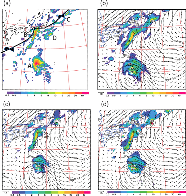
 denotes a front. (b) The mean of the 14-h CRM ensemble forecasts starting at 00 UTC, September 7, 2015, for precipitation in mm h−1 (shade), pressure in hPa (contours), and horizontal winds at surface in m s−1 (arrows). (c) The same as (b) but for the mean of the 14-h CRM ensemble forecasts starting at 00 UTC, September 7, 2015, after DEC. (d) The same as (b) but for the mean of the rainy regime of the 14-h CRM ensemble forecasts starting at 00 UTC, September 7, 2015, after DEC. The color bar is surface precipitation in mm h−1. Cross (x) denotes the typhoon centers obtained from the best track data. Pluses (+) denote points with the minimum ensemble-mean surface pressure.
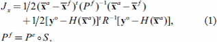


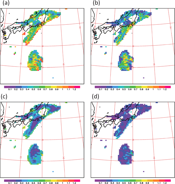
 (dimensionless) of surface precipitation for the PDF models calculated from 14-h CRM ensemble forecasts starting at 00 UTC, September 7, 2015, after DEC. (a) For the N model. (b) For the MN model. (c) For the LN model. (d) For the MLN model. The color bars are
  (dimensionless).


 denotes a front. (b) The analyses given by FG for precipitation in mm h−1 (shade), pressure in hPa (contours), and horizontal winds at surface in m s−1 (arrows). The color bars are surface precipitation in mm h−1. (c) The same as (b) but by CN. (d) The same as (b) but by GD. (e) The same as (b) but by MLD. (f) The same as (b) but by SD. The color bars are surface precipitation in mm h−1.
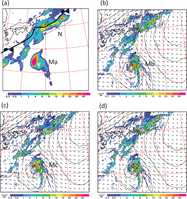
 denotes a front. (b) The same as