Abstract
The Global Precipitation Measurement (GPM) Dual-frequency Precipitation Radar (DPR) has operated in full scan (FS) mode in both the Ku-band and Ka-band since May 2018. This FS mode can enable about 245 km full swath dual-frequency processing for the first time, whereas previous algorithms enabled dual-frequency processing in the narrower inner swath, having a width of approximately 125 km. This paper describes the classification (CSF) module in newly developed DPR level 2 V06X experimental algorithms corresponding to the FS mode. The CSF module classifies precipitation as three major types, stratiform, convective, and other, and provides bright-band (BB) information.
One-month statistics show that a significant jump occurs in the Ka-band precipitation type counts at the edges of the inner swath due to the different sensitivity of Ka-band radar in Ka-band Matched Scan (Ka-MS) mode compared with that in Ka-band High Sensitivity (Ka-HS) mode. However, precipitation type counts indicate that dual-frequency processing works well not only in the inner swath but also in the outer swath. Statistics on BB counts show a significant improvement in BB detection, especially in the outer swath, when dual-frequency processing is performed.
In addition, the V06X Ku-band algorithm solves two problems related to the CSF module: (a) appearance of a very large near-surface precipitation rate of stratiform precipitation reclassified by the slope method and (b) a rare case of misjudging BB peak as an upper part of surface echo.
The data structures of GPM DPR algorithms were drastically changed in V06X. The new data structures introduced in V06X will be used in V07A and later. In this regard, the V06X CSF module outlined in this paper is a prototype of future versions of each CSF algorithm.
1. Introduction
Dual-frequency Precipitation Radar (DPR) is operating in the Ku-band and Ka-band at the core observatory of the Global Precipitation Measurement (GPM) mission (Kojima et al. 2012; Hou et al. 2014; Kubota et al. 2014; Skofronick-Jackson et al. 2017; Iguchi 2020; Nakamura 2021). The GPM core observatory was launched into orbit on February 28, 2014 (Japan Standard Time). It flies in a non-Sun-synchronous orbit, and observes precipitation in the latitude ranging from 65°N to 65°S. Furthermore, the GPM core observatory comprises two sensors: DPR and GPM Microwave Imager (GMI) (Hou et al. 2014; Skofronick-Jackson et al. 2017).
The Ku- and Ka-band radars have almost the same antenna beam shape and observe precipitation with the same footprint size, which is approximately 5.2 km at the nadir. The pulse width of the Ku-band radar is 1.6 µs, and the range resolution is 250 m. The Kaband radar operates with two pulse-widths: 1.6 µs and 3.2 µs (Kojima et al. 2012; Iguchi et al. 2020). In the Matched Scan (MS) mode, the Ka-band radar operates with the 1.6 µs pulse-width, making the range resolution 250 m. In the High Sensitivity (HS) mode, the Ka-band radar operates with the 3.2 µs pulse-width that makes the range resolution 500 m. The sensitivity of Ka-band radar in HS mode operation is higher than that of MS mode operation because the energy contained in a radar pulse becomes larger as the radar pulse-width increases. Thus, the Ka-band radar in HS mode operation achieves high sensitivity at the expense of range resolution.
There are three DPR level 2 (L2) algorithms that output physical data derived from the DPR level 1 engineering data: there are two single frequency (SF) algorithms and one dual frequency (DF) algorithm. Each algorithm consists of modules (Iguchi 2020; Iguchi et al. 2020). The DF algorithm is applicable only when the radar beam of Ku-band radar and that of the Ka-band radar match. Notably, radar beam matching is essential for applying the DF algorithm; if the range resolutions are different, interpolated data can be used for the DF processing.
Until May 21, 2018 (approximately 1600 UTC), the Ka-band radar observed precipitation in a narrow inner swath of about 125 km with two antenna scan modes called Ka-band Matched Scan (Ka-MS) mode and Ka-band High Sensitivity (Ka-HS) mode, whereas the Ku-band radar observed precipitation in a full swath of approximately 245 km. The DF algorithm modules only processed the inner swath data until May 21, 2018.
Figure 1a displays the antenna scan pattern of DPR before May 21, 2018. The Ku-band radar scanned the radar beam in a cross-track direction by pointing its beam in 49 directions. In one antenna scan, each antenna beam direction is specified by a quantity called angle bin number, which takes values from 1 to 49. The full swath data consist of 49 angle bin data. At angle bin number 25, the antenna beam points to the nadir. In this paper, the angle bin number is counted with respect to that of the Ku-band radar.
The Ka-band radar observed precipitation in the inner swath whose angle bin number ranges from 13 to 37 where the antenna beam of Ka-band radar and that of Ku-band radar were matched. However, when the Ku-band radar observed precipitation in the outer swath, which can be specified by angle bin numbers 1–12 and 38–49, the Ka-band radar observed precipitation in HS mode in the inner swath whose angle bin number takes a half-integer ranging from 13.5 to 36.5. Therefore, the Ka-HS mode and the Ku-band antenna beams were not matched.
On May 21, 2018, the antenna scan pattern of the Ka-band radar was changed to observe precipitation in the outer swath in Ka-HS mode. Figure 1b shows the antenna scan pattern of DPR after the Ka-band antenna scan pattern change. After May 21, 2018, the Ka-band radar also observes precipitation in the full swath, with its antenna beam being matched with the Ku-band beam (Iguchi 2020; Iguchi et al. 2020). Thus, at the cost of abandoning the Ka-HS mode observation of precipitation in the inner swath, full swath data for DF processing have been available since May 21, 2018. However, as far as the DF data are concerned, the current DPR L2 algorithms version 06A (V06A) released in October 2018 could only process the inner swath DF data, but not the full swath DF data. Thus, the current V06A algorithms continue to process data after the Ka-HS antenna scan pattern was changed by assuming that Ka-HS data are missing. Conversely, full swath DF processing is performed by the newly developed DPR L2 V06X experimental algorithms, which were released in June 2020. Consequently, the DPR L2 V06X algorithms are only applicable to data obtained after the Ka-HS antenna scan pattern was changed, but the subsequent V07A algorithms planned to be released in 2021 can handle data obtained both before and after the modification to the Ka-HS antenna scan pattern.
The DPR L2 algorithms consist of several modules (Iguchi et al. 2020), including the classification (CSF) module, where precipitation is classified into three major types: stratiform, convective, and other (Awaka et al. 2016). The paper's primary purpose is to show how the V06X CSF module handles the full swath Ka-band data. This paper shows for the first time what the full swath statistics of the Ka-band and DF precipitation type counts look like.
The rest of this paper is arranged as follows. Section 2 describes the data structures and overviews the algorithms in V06A and V06X. Next, Section 3 outlines the V06X CSF modules, and Section 4 presents CSF-related V06A problems mitigated in V06X. Notably, Section 5 highlights the statistical results of V06X CSF output data. Finally, Section 6 summarizes the conclusion and addresses future work.
2. Data structures and overview of algorithms in V06A and V06X
Figure 2 exhibits the data structures of the current V06A and new experimental V06X DPR L2 algorithms. Both V06A and V06X algorithms consist of two single frequency (SF) algorithms (i.e., Ku- and Ka-band algorithms) and one DF algorithm. In V06A shown in Fig. 2a, the Ku-band SF algorithm outputs Ku-band Normal Scan (Ku-NS) data, the Ka-band SF algorithm outputs Ka-MS and Ka-HS data, and the DF algorithm outputs DPR-NS, DPR-MS, and DPR-HS data. Only Ku-NS and DPR-NS are full swath data, while the rest are inner swath data. Though DPR-NS data consist of full swath Ku-band-related data, DF processed data can only be found in the inner swath portion of the DPR-NS data. The current DPR L2 V06A algorithms continue to process the data obtained after the Ka-band antenna scan pattern was changed on May 21, 2018, but with the Ka-HS and DPR-HS data missing. In V06X, the SF and DF algorithms output full swath Ku-FS and Ka-FS as well as DPR-FS data, respectively, as shown in Fig. 2b. The Ka-FS data are obtained in MS mode in both inner and outer swaths. Therefore, “MS mode” in Fig. 2b should be understood as a shorthand notation for “normal sensitivity inner swath MS mode” and “HS mode” for “HS outer swath MS mode”. The DPR L2 V06X algorithms are the first ones that process the full swath data obtained after the Ka-HS antenna scan pattern was changed on May 21, 2018. Though not used in V06X, the DPR L2 V06X algorithms prepare Ka-HS and DPR-HS data structures so that the algorithms can handle the data obtained before the Ka-HS antenna scan pattern was changed.


Figure 3 shows the data flow of the V06A (or V06X) Ku-band SF algorithm that handles Ku-NS (or Ku-FS) data. The Ku-band SF algorithm consists of the preparation (PRE) module, vertical profile (VER) module, CSF module, drop size distribution (DSD) module, surface reference technique (SRT) module, and solver (SLV) module (Iguchi et al. 2020). The PRE module provides the measured radar reflectivity factor, precipitation/no-precipitation classification, and clutter mitigation (Kubota et al. 2016). The VER module computes the path-integrated attenuation (PIA) due to nonprecipitation particles (piaNP) and generates a radar reflectivity factor corrected for piaNP (Kubota et al. 2020). The CSF module classifies precipitation types and obtains BB information. This study focuses on the CSF module, which is later described in detail. The SRT module estimates PIA for precipitation pixels (Meneghini et al. 2015). Finally, the SLV module numerically solves the radar equations and obtains DSD parameters and precipitation rates at each range bin (Seto et al. 2013, 2021; Seto and Iguchi 2015).
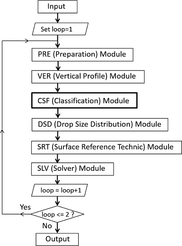
The Ku-band SF algorithm has a loop structure, and the data go through the modules within the loop twice. In other words, the data return to the start point of the loop only once.
The data flow of the Ka-band SF algorithm is the same as that shown in Fig. 3 except for the fact that the starting point of the loop is after the PRE module in the Ka-band SF algorithm. In the V06A algorithms, Ka-MS data and Ka-HS data are separately processed by a data flow similar to that shown in Fig. 3. In V06X algorithms, Ka-FS data are processed by a data flow similar to that shown in Fig. 3.
The data flow of the DF algorithm is the same as that shown in Fig. 3 but without the loop structure. In the V06A CSF module, the DF processing developed based upon Le and Chandrasekar (2013a, b) is applied to the combination of Ka-MS and the inner swath of the Ku-NS data and to the combination of Ka-HS and the corresponding interpolated Ku data, respectively. In the V06X CSF module, however, updated DF processing is applied to the combination of Ka-FS and the corresponding Ku-FS data. New output items related to the V06X CSF module are summarized in Appendix.
3. Overview of the V06X CSF modules
In the GPM DPR L2 V06X algorithms, there are three CSF modules: two SF CSF modules (Ku-FS CSF module and Ka-FS CSF module) and one DF CSF module (DPR-FS CSF module). The main purposes of the CSF modules are to detect bright band (BB) and classify precipitation as three major types: stratiform, convective, and other.
Figure 4 shows the precipitation type decision flow in the Ku-FS CSF module, which includes two main methods for precipitation type classification: the vertical profiling method (V-method) and the horizontal pattern method (H-method) (Awaka et al. 2009, 2016). The precipitation type decision is completed on a “pixel” basis so that a precipitation type is given to each antenna beam as a whole (i.e., does not change along the antenna beam), and each antenna beam is mapped to each corresponding pixel.

BB is detected first in the V-method because its existence is a good indicator of stratiform precipitation (Battan 1973; Houze 1993). The V-method can detect BB because BB can be characterized by a unique, strong peak near the freezing height in the height profile of the radar reflectivity factor (Z) near the freezing height (Klaassen 1988; Fabry and Zawadzki 1995). In the V-method, detection of BB is made by a peak search of Z in a BB search window determined by the height of the 0°C isotherm. The 0°C height is estimated in the VER module using the global analysis data (GANAL) of the Japan Meteorological Agency (JMA) (Kubota et al. 2020). The BB search window is from 0°C height − 2 km to 0°C height + 1 km. This choice of BB search window is based on a statistical finding by the Tropical Rainfall Measuring Mission (TRMM) precipitation radar that the BB peak appears about 0.5 km below the 0°C height on average (Awaka et al. 2009). Rigorously speaking, what is used in the detection of BB is Z-factor corrected for attenuation by nonprecipitation (NP) particles, ZNPcorrected (Iguchi et al. 2020).
The V-method also examines ZNPcorrected along the antenna beam. The V-method makes the following decision on the precipitation type of the pixel being considered. (1) If BB is detected, the precipitation type is basically stratiform but is convective when ZNPcorrected of precipitation close to the surface is exceptionally strong (i.e., when ZNPcorrected > 46 dBZ). (2) If BB is not detected, then ZNPcorrected of precipitation echo along the antenna beam is examined. If the maximum value of ZNPcorrected along the beam exceeds the convective threshold (set to 40 dBZ), the precipitation type is convective. (3) If the precipitation type is neither stratiform nor convective, the precipitation type obtained by the V-method is other.
Table 1 summarizes the V-method and also lists the percentages of each precipitation type for July 2020. The main target of the V-method is the detection of stratiform precipitation that accompanies detectable BB. Another target of the V-method is the detection of strong convective precipitation. But the above two targets do not cover all cases. The table lists 76.9 % of precipitation types as being other, which means that precipitation types of a large number of precipitation pixels are left undecided. The following H-method clears this indecisive situation.

Based on the University of Washington convective/stratiform separation method (Steiner et al. 1995; Yuter and Houze 1997), the H-method examines the horizontal pattern of Zmax (i.e., maximum value of ZNPcorrected along the antenna beam in the rain region), which means Zmax is obtained from ZNPcorrected below the BB region when BB exists. The reason why the CSF module uses Zmax is as follows. The University of Washington convective/stratiform separation method was developed for analyzing the data obtained by a ground-based radar to classify precipitation into two categories, and the method examines the horizontal pattern of Z at a given height. To examine Z at a given height is appropriate for ground-based radars, but it is inappropriate for the GPM DPR because it observes precipitation over the ocean and land. Over the ocean, it would be easy to examine Z at a given height by the DPR. However, it would become impossible for the DPR to select the appropriate data height over land when it observes precipitation over very high mountain regions. Nevertheless, it is requested that the DPR analyze the data over high mountain regions and decide on precipitation types. In order to solve this problem, the H-method in the CSF module uses Zmax in place of Z at a given height.
The main target of the H-method is the detection of the convective type. Thus, the H-method starts with the detection of a convective center.
When either of the following conditions is satisfied, the pixel being considered is judged to be a convective center.
-
(1) Zmax of the pixel exceeds the convective threshold (which is 40 dBZ in V06X); or
-
(2) Zmax of the pixel stands out against those in the surrounding background area.
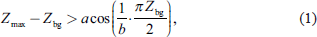
In (2), Zmax is compared with Zbg, an average value of Zmax in a surrounding background area. If the following inequality is satisfied, then it is said that Zmax satisfies the stand-out condition:
where
a and
b are parameters. The analytical formula on the right side of
Eq.(1), described in
Yuter and Houze (1997), can reasonably approximate the formula given by
Steiner et al. (1995). Since the right side of
Eq.(1) is continuous, it is easy to use. The parameter values used in the Ku-band H-method are
a = 9.0 and
b = 43.75. For simplicity, those values are also used in the Ka-band H-method.
The precipitation type of the convective center is convective, and the precipitation type of four pixels adjacent (not diagonally) to the convective center is also convective when the adjacent pixel is a precipitation pixel. When not convective, the H-method precipitation type is stratiform if Zmax exceeds a predetermined noise threshold. Otherwise, it is other. Thus, the other type obtained by the H-method means a case where ZNPcorrected in the rain region is noise (e.g., realized in case of clouds only). The introduction of the other category is needed for the H-method because it should handle the case when there is no precipitation on the surface, but there is precipitation in the upper region. The noise threshold used in the Ku-FS H-method is 12.0 dBZ. For simplicity, the noise threshold of 15.0 dBZ is used in the Ka-FS H-method for both inner and outer swath. However, a smaller threshold value should be used in the outer swath where Ka-band radar operates in HS mode, which is an issue for V06X.
The V-H precipitation type is obtained as follows from the V- and H-method precipitation types:
-
(1) When the V-method precipitation type is stratiform, the V-H precipitation type is stratiform because BB is detected by the V-method.
-
(2) When the V-method precipitation type is convective, the V-H precipitation type is convective because Z is strong.
-
(3) When the V-method precipitation type is other, the H-method precipitation type is the V-H precipitation type.
Table 2 summarizes the V-H precipitation type with percentages obtained by using the July 2020 V06X data. Through process (3) above, the V-method other type that occupies 76.9 % of precipitation pixels in the July 2020 V06X statistics (see Table 1) is broken down into 64.3 % stratiform, 7.3 % convective, and 5.3 % other. Thus, the overall percentage of the V-H precipitation types are 83.9 % stratiform, 10.8 % convective, and 5.3 % other.
As shown in Fig. 4, the V-H precipitation types undergo unification by consulting the results of small size precipitation detection, shallow rain detection, and Heavy Ice Precipitation (HIP) detection. But the V-H other type is not affected by the unification; if the V-H precipitation type is other, then the unified precipitation type is other even when a small size cell, shallow rain, or HIP is detected.
Small-sized precipitation is defined as (a) a single precipitation pixel surrounded by no-precipitation pixels or (b) two adjacent precipitation pixels surrounded by no-precipitation pixels. The type of smallsized precipitation could not be stratiform because the smallness of the precipitation size disagrees with the wide-spreading nature of stratiform precipitation. Therefore, if small-sized precipitation is detected, the unified type of small-sized precipitation is convective when the V-H precipitation type is not other. Small-sized precipitation was detected in 2.6 % of V06X Ku-FS precipitation pixels in July 2020.
Shallow rain is defined as precipitation whose storm top height is lower than the freezing level height by at least 1 km (Awaka et al. 2016; Iguchi et al. 2020). When shallow rain is detected, the unified precipitation type is convective when the V-H precipitation type is not other. Shallow rain was detected in 9.1 % of V06X Ku-FS precipitation pixels in July 2020.
Iguchi et al. (2018) conceived the idea of HIP. Since version 05 (V05) was released in May 2015, the CSF modules have been looking for HIP in the upper region of a storm where the temperature is lower than −10°C. The definition of HIP is different for Ku-, Ka-, and DPR-data processing, as listed in Table 3. For Ku-FS data, HIP is defined as precipitation consisting of ice particles that produce a large measured Z factor (Zm) (i.e., Zm > 35 dBZ). If HIP is detected, the unified precipitation type is essentially convective. However, if the V-H precipitation type is stratiform because of BB being detected, the unified precipitation type is stratiform even when HIP is detected. In this case, the upper ice region is convective because of the detected HIP, but the lower rain region is stratiform because of the detected BB. For the purpose of precipitation rate retrieval, the precipitation type in the lower precipitation region matters; therefore, the unified precipitation type is stratiform in this case. If the V-H precipitation type is other, then the unified precipitation type is other even when HIP is sensed. HIP was detected in 0.5 % of V06X Ku-FS precipitation pixels in July 2020.

Houze and Brodzik (2017, private communication) noticed that the V05 Ku-band CSF module incorrectly classified many stratiform pixels as convective pixels. They developed a “slope” method to solve the problem. The method examines the Z profile above the 0°C isotherm for convective precipitation, and if the slope resembles that in the upper part of BB, the convective type is reclassified as the stratiform type. As shown in Fig. 4, the slope method is implemented in the last part of the V06X Ku-FS CSF module. The slope method was first introduced in the V06A Ku-NS CSF module, whose data flow is the same as shown in Fig. 4.
The V06X Ka-FS CSF module has the same data flow as shown in Fig. 4, except that there is no slope method in the Ka-band module. The reason why the V06X Ka-FS CSF module does not include the slope method is because the strong rain attenuation of the Ka-band makes the detection of convective type infrequent, and there is no need to reclassify convective type to stratiform by the slope method. The slope method is considered most necessary in the outer swath where the BB peak smears and some BB peaks may be masked by smeared surface clutter. In the inner swath, strong Ka-band rain attenuation and slightly lower sensitivity of the Ka-MS mode radar reduce the chances of detecting convective type, so that reclassification from the convective type to stratiform by the slope method is unnecessary. Notably, the slope method is introduced to solve the problem of too many convective type counts in the V06A Kuband data. This problem originates from the fact that the V-method does not detect some smeared BBs. If the smeared BB is not identified, then the type is not decided as stratiform, and the V-method proceeds to examine ZNPcorrected along the entire radar beam. Furthermore, if the peak value of ZNPcorrected exceeds the Ku-band convective threshold, then the V-method decides that the type is convective though, in reality, it is stratiform because there is the smeared BB that the V-method fails to detect. The slope method remedies this problem by examining the slope of ZNPcorrected above the 0°C isotherm. In the case of Ka-band data, however, a large attenuation makes the peak values of ZNPcorrected small. Therefore, the chances of ZNPcorrected exceeding the convective threshold are small even when the Ka-band V-method fails to detect a smeared BB. Thus, in the case of Ka-band, precipitation type for missed BB would mostly be stratiform. Notably, the V06A Ka-MS data do not exhibit the “too many convective type” problem. However, the next version of the Ka-FS CSF module includes the slope method if necessary since the Ka-FS mode is a full swath mode and has high sensitivity data in the outer swath.
The DPR-FS CSF module uses the method developed based upon Le and Chandrasekar (2013a, b) of Colorado State University (CSU). Their method is based on using the measured Dual-frequency Ratio (DFRm) for precipitation type classification. The definition of DFRm is as follows:
where
Zm (Ku) and
Zm (Ka) are the measured
Z (in dB) in the Ku-band and Ka-band, respectively. This paper calls Le and Chandrasekar's method the CSU DFRm method to differentiate it from any other method that also uses DFRm. The CSU DFRm method not only classifies precipitation types but also detects melting layer (ML) boundaries. The ML concept has a wider meaning than BB in a sense that BB is a subset of ML because the melting of solid particles causes BB and because ML exists in both stratiform and convective precipitations. In the case of stratiform precipitation, ML can be identified with BB.
Figure 5 shows an example of the DFRm height profile that shows a clear “bump” near the 0°C isotherm. The figure shows key points B and C for the CSU DFRm method. At point B, DFRm takes a local maximum value, and at point C, DFRm takes a local minimum value.

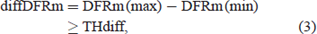
The CSU DFRm method is applied to the precipitation pixel where both Ku-band and Ka-band precipitation echoes exist. When these DF precipitation echo data exist, then the CSU DFRm method examines precipitation echo data in a possible ML region near the 0°C isotherm. Here, the possible ML region means the height region between 0°C height - 2 km and 0°C height + 1 km, where 0°C height is the estimated height obtained by using the GANAL data. If there is not enough precipitation echo data in the possible ML region, then the CSU DFRm method skips the processing. If not skipped, then the CSU DFRm method looks for the points B and C, defined in Fig. 5, of the DFRm “bump” in the possible ML region. It is requested that the following condition is satisfied:
where DFRm (max) is the DFRm value at point B, DFRm (min) is located at point C, and THdiff is a threshold. In V06X, THdiff = 2.0. If points B and C are determined, which satisfy the above
Eq.(3), then the following quantities (i.e.,
V1 and
V2) are calculated. The definition of
V1 is
where DFRmLIN(max) is the linear value of DFRm at point B, and DFRmLIN(min) is the linear value of DFRm at point C. By
Eq.(4), the difference DFRm (max) - DFRm (min) is mapped to
V1 because
V1 is uniquely determined by DFRmLIN(max)/DFRmLIN(min), and this mapping is one-to-one. In
Eq.(4), the linear value of DFRm is used so that
V1 is guaranteed only to take on a value between zero and one.
The definition of V2 is
where DFRm in the rain region corresponds to DFRm below point C (see
Fig. 5), and the slope is measured with respect to height in km. If
V2 is smaller than 0.5 dB km
−1, then the DFRm processing is skipped. Otherwise, the following
V3 is calculated.
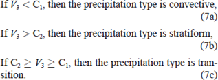
The CSU DFRm method determines precipitation type by the following rule:
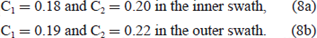
In the above, C1 and C2 are empirical parameters and take the following values:
After the precipitation type decision, the CSU DFRm method performs ML detection. First, the CSU DFRm method examines the DFRm profile exhibiting the “bump” that satisfies Eq.(3). In this examination, if a point where the absolute value of the DFRm slope becomes largest is found in the possible ML region then the point is judged as the ML top, and point C is regarded as the ML bottom.
As shown in Fig. 6, as the CSU DFRm method alone could not handle all precipitation cases, the V06X DPR-FS CSF module also uses the Ku-FS results (or Ka-FS results when Ku-FS results are not available) for determining unified precipitation types. The CSU DFRm method classifies precipitation into three types: stratiform, convective, and transition. If the CSU DFRm precipitation type is transition, the Ku-FS CSF decision is used for the unified precipitation types. The precipitation types by the CSU DFRm method are 7.6 % stratiform, 2.6 % convective, and 0.6 % transition in the July 2020 V06X statistics.
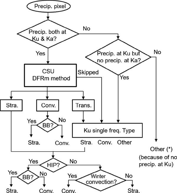
As shown in Fig. 4, the Ku-FS CSF module performs additional decisions on small-sized precipitation, shallow rain, and HIP. In the V06X DPR-FS CSF module, small-sized precipitation and shallow rain decisions are copied from the Ku-FS CSF module but not from the Ka-FS CSF module because a large Ka-band rain attenuation and a lower sensitivity of Ka-band data, particularly in the inner swath, cause unreliable Ka-FS results on small-sized precipitation and shallow rain. On the other hand, however, the V06X DPR-FS CSF module adds a DFRm decision to HIP (see Table 3). The HIP decision is made at a later part of the flow, as shown in Fig. 6. Furthermore, a winter convection detection that examines DFRm at and around the storm top follows after the HIP decision and examines whether HIP exists nearby (see Iguchi et al. 2020 for details). The V06X DPR-FS CSF module uses the HIP information and winter convection detection results to produce the final outcome of unified precipitation types. Incidentally, the addition of the DFRm decision to HIP is also made in V06A.
The right hand side of Fig. 6 indicates that precipitation type is other if the condition “precipitation at Ku but no precipitation at Ka” is not satisfied, which is a bug. If this condition is not satisfied, Ka-band single frequency precipitation type should be used instead of other. The effect of this bug is apparent as shown later in Fig. 11. The bug is fixed in V07A.
4. CSF-related V06A problems mitigated in V06X
There are two significant CSF-related problems in the standard V06A products: one concerns the slope method and the other concerns the detection of a clutter-free bottom in the PRE module that affects BB detection and is thus CSF-related. The V06X algorithms solve both problems.
4.1 Improvement of the slope method
The slope method examines the Ku-band Z profile of convective precipitation. When the absolute value of the slope of ZNPcorrected relative to height is very large above the 0°C isotherm, the convective type is reclassified as the stratiform type. The slope method is implemented in the V06A (and V06X) Ku-band CSF module.
Immediately after the release of V06A data, the near-surface precipitation rate (PNS) of the reclassified stratiform type was found to sometimes become very high because the V06A slope method only examines the height region above the 0°C isotherm. However, it is difficult to imagine that stratiform precipitation accompanies a very high precipitation rate near the surface. Therefore, to solve this problem, a limit was set on the slope method's input so that the technique could be applied to convective precipitation whose PNS is smaller than a threshold, which is 20 mm h−1 in V06X (Awaka and Brodzik 2019). The idea behind this is as follows: if convective precipitation having a smaller PNS were reclassified as stratiform, the PNS of the reclassified stratiform precipitation would also be small.
Figure 7 displays the PNS of the reclassified stratiform precipitation in the form of a histogram. The figure is based on July 2020 data. Figure 7a shows the histogram of PNS obtained by the V06A slope method and clearly shows that the reclassified stratiform precipitation produces appreciable numbers of large PNS (> 50 mm h−1). Figure 7b shows the corresponding histogram obtained by the improved V06X slope method. In Fig. 7b, the large PNS (> 50 mm h−1) disappears. Therefore, it can be concluded that the improved V06X slope method works well. However, though the threshold of 20 mm h−1 is introduced into the V06X slope method, Fig. 7b shows that the PNS of the reclassified stratiform precipitation still exceeds the threshold in a small number of cases. The following explains this behavior.
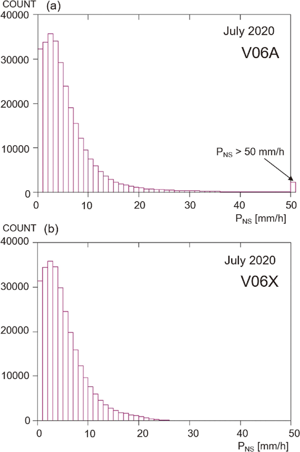
As shown in Fig. 3, since the CSF module is placed in an earlier part of the flow in the loop, the CSF module can use PNS obtained by the SLV module in the 1st loop [PNS (1st loop)] but not that obtained in the 2nd loop [PNS (2nd loop)]. Users can use PNS (2nd loop) but not PNS (1st loop) because the latter is an internal quantity. The PNS quantity in Fig. 7 is PNS (2nd loop). Furthermore, the non-uniform beam filling (NUBF) effect (Seto et al. 2021) is included in the SLV module in the 2nd loop but not in the 1st loop. Consequently, PNS (2nd loop) can generally become greater than PNS (1st loop). In the V06X slope method, a limit is imposed on PNS (1st loop) because the method could not access PNS (2nd loop). Therefore, in Fig. 7b, PNS (2nd loop) may sometimes exceed the limit imposed on PNS (1st loop).
4.2 Improvement in the decision on a clutter-free bottom
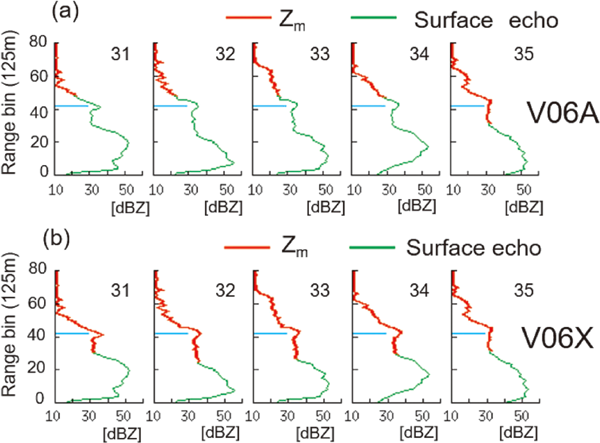
Due to a bug in the Ku-band V06A PRE module, a few cases occur where a BB peak is misjudged as the upper part of surface echo. When this happens, a clutter-free bottom is falsely set at an altitude higher than the BB peak height, which eliminates the opportunity to observe BB and rain below BB. This problem has thus far been found in the following two cases: (a) high BB case and (b) low BB case.
a. High BB case
The problem mentioned above can be found in the V06A data over mountainous areas where the surface echo takes a complicated and broadened shape. Figure 8 shows examples where the profile of Ku-band Zm is plotted for a few angle bins. Figure 8a shows some V06A Zm profiles where each BB at angle bin numbers 31–34 is regarded as a part of surface echo. Figure 8b shows the bug-fixed V06X results that clearly distinguish BB from the surface.
b. Low BB case
The problem mentioned above could occur near nadir in winter when BBs appear very close to the surface. Notably, Watters et al. (2018) reported this problem. Figure 9 shows Ku-band Zm profiles for low BB, where Fig. 9a shows the Zm profiles before the bug fix (V06A), and Fig. 9b shows those after the bug fix (V06X).
5. Statistical results
Figure 10 shows one-month (July 2020) statistics on precipitation type counts obtained by the V06X single frequency modules: Ku-FS and Ka-FS results are shown by thin and thick lines, respectively. The abscissa shows the angle bin number, which indicates the antenna beam direction within one antenna scanning plane that is perpendicular to the direction of satellite movement; the angle bin number 25 corresponds to the nadir direction. The figure shows that among the counts of three major precipitation types for both Ku-FS and Ka-FS, the stratiform count is the largest, followed by the convective count and then the other count. Notably, each type count of Ka-FS exhibits a stepwise change at both edges of the inner swath because the Ka-band radar operates in low-sensitivity Ka-MS mode in the inner swath, but the radar operates in high sensitivity Ka-HS mode in the outer swath (Masaki et al. 2020).
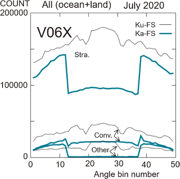
Though unclear in the figure, the other type count of Ka-MS is not zero. The other count of Ka-MS in the figure is approximately 1000 for each angle bin in the inner swath. We simply interpret that this occurs because the low sensitivity of Ka-MS makes the detection of weak precipitation very difficult. Surprisingly, the other type count of Ka-HS is larger than that of Ku-FS in the outer swath. We think this occurs because the noise threshold for the Ka-HS is 15.0 dBZ, which is the value used for Ka-MS. Since the Ka-HS data is obtained by HS mode operation, the noise threshold for the Ka-HS should be smaller than 15.0 dBZ. This is a parameter tuning issue, and V07A data is processed using appropriate parameters.
Figure 10 also indicates the following very interesting fact. If we add up all three type counts at each angle bin, we obtain the precipitation count at each angle bin because precipitation consists of three types of precipitation. Then we can conclude that the precipitation counts of Ku-FS data are higher than those of Ka-HS data. However, it is reported that the sensitivity of HS mode Ka-band radar is higher than that of Ku-band radar (Masaki et al. 2020). Though HS mode Ka-band radar has higher sensitivity, its precipitation counts are lower than Ku-band radar. The main reason for this would be that the radars observe not only rain but also ice and snow. If the radars observe only rain, the HS mode Ka-band radar would observe weaker rain that the Ku-band radar cannot detect. However, the situation is different for the observation of ice and snow. Liao and Meneghini (2011) showed that the reflectivity of solid particles at Kaband could be smaller than that at Ku-band by more than a few dB. There may be other reasons, but Liao and Meneghini's findings may be the main reason that the Ku-band radar can detect precipitation more than the higher sensitivity Ka-band radar. The strong attenuation at the Ka-band would not be the reason for the higher precipitation count of Ku-FS radar because strong attenuation is caused by moderate or intense rain, then the upper part of such precipitation should be observed by both Ka- and Ku-band radars.
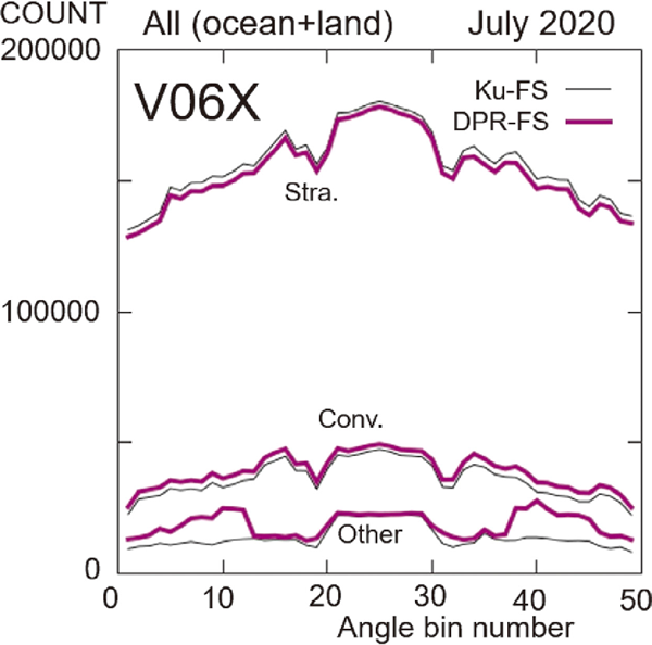
The angle bin dependence of each unified precipitation type count obtained by the V06X DPR-FS CSF module (thick lines) is shown in Fig. 11. The thin lines plot the corresponding Ku-FS results for comparison. Compared to the Ku-FS results, the DPR-FS stratiform count is slightly lower (almost parallel-shifted downward), whereas the DPR-FS convective count is slightly higher (almost parallel-shifted upward). The almost parallel-shift behavior observed above in stratiform curves and convective curves indicate that the CSU DFRm method works well in the outer swath. This finding is important because the CSU DFRm method is applied to the outer swath data for the first time in V06X.
Figure 11 shows that the DPR-FS other type count is much greater than the corresponding Ku-FS count in the outer swath because of the V06X bug described at the end of Section 3. When the bug is fixed, the bump of the other count by DPR-FS disappears, and stratiform and convective counts by DPR-FS slightly increase in the outer swath. The bug fix is made in V07A.
Figure 12 is essentially the same as Fig. 11 but shows the statistics separately over the ocean and land. The general trend of the curves in Fig. 12a is almost the same as that in Fig. 12b, although the statistics shown in Fig. 12a have larger counts than those in Fig. 12b; nothing strange seems to occur over the ocean or land. This fact implies that the CSF module V06X works well over ocean and over land.
Incidentally, Fig. 12 shows that the difference of each type count between Ku-FS and DPR-FS over land is smaller than that over the ocean. However, care should be taken that precipitation statistics over land are susceptible to sampling errors and seasonal biases.
Figure 13 depicts the angle bin dependence of the BB counts obtained by the V06X Ku-FS CSF module (thin line) and the V06X DPR-FS CSF module (thick line). The advantage of DF processing is evident, particularly in the outer swath, as shown by the thick line.
Table 4 summarizes the improvement of BB detection because of the introduction of DF processing. The following quantity assesses the enhancement:
where A is the BB count obtained by the V06X Ku-FS CSF module, and B is the BB count obtained by the V06X DPR-FS module. The table shows the 22.1, 12.0, and 68.9 % improvement in the full, inner, and outer swaths, respectively, confirming the advancement of BB detection in the outer swath using DF processing in the outer swath.

In the V06X DPR-FS CSF module, the CSU DFRm method makes an “extension” to ML detection. The detection of ML can be made by THdiff, whose value is different from the value used to determine precipitation type. If ML is not detected using THdiff = 2.0, which is used to find the precipitation type, the ML detection is attempted using THdiff = 0.5. The “extension” means that the detection of ML is made using THdiff = 0.5. In V06X, the information about whether ML is detected by the “extension” or not is given to a quality flag. From Eq.(3), it is understood that the use of a smaller value of THdiff means the detection of ML is made for the data showing less clear DFRm “bump”, signifying that the reliability of ML detected by the “extension” could be low. Consequently, a trial to identify ML as BB is not performed for the ML detected by the “extension” in V06X. Introducing a BB identification process for ML detected by the “extension” would increase the number of detected BBs, but this is a matter for V07A.
6. Conclusions
This paper described the CSF modules in GPM DPR L2 V06X that were released in June 2020. The V06X algorithms were developed to process full swath Ka-band data that have been obtained since May 18, 2018, when the antenna scan pattern of the Ka-band radar was changed.
The following problems related to the CSF module are solved in the V06X Ku-band algorithm: (a) appearance of a very large near-surface precipitation rate (PNS) of stratiform precipitation reclassified by the slope method and (b) a rare case of misjudging BB peak as an upper part of surface echo.
One-month statistics show that a significant jump occurs in the Ka-band precipitation type counts at the edges of the inner swath because the sensitivity of Ka-band radar in Ka-MS mode differs from that in Ka-HS mode. In the V06X DPR-FS CSF module, the CSU DFRm method is applied to DF data in the outer swath for the first time. The statistics show that the CSU DFRm method works well not only in the inner swath but also in the outer swath. The statistics also show a considerable improvement in BB detection in the outer swath when using DF data.
The following two tasks are also undertaken as part of algorithm development for V07A to be released in 2021.
(1) Improvement of BB detection in both SF and DF modules
This is a long-standing issue. An interesting possibility of improving BB detection in the DF CSF module is related to “MixedPhaseTop” in Appendix.
(2) Re-examination of weak stratiform precipitation not accompanying BB
This is also a long-standing issue. If BB is not detected, some stratiform precipitation determined by the current CSF module may be convective, which can occur in winter data, for example. Studies on this issue should be continued.
Acknowledgments
This work is a result of the Precipitation Measurement Mission (PMM) of the Japan Aerospace Exploration Agency (JAXA) and the National Aeronautics and Space Administration (NASA). One of the authors, Jun Awaka, wishes to thank Prof. T. Ushio of Osaka University for making the work possible by allowing the author to be his co-investigator in JAXA's research program on PMM.
Appendix: New output items related to the CSF module in DPR L2 V06X
This appendix briefly describes the new output items of the V06X CSF modules. Details can be found in Iguchi et al. (2020).
A.1 Additional information about Heavy Ice Precipitation (HIP)
In V06X, the following new items relating to HIP were introduced to present information about the ranges where HIP is detected.
-
a) binHeavyIcePrecipTop
-
b) binHeavyIcePrecipBottom
-
c) nHeavyIcePrecip
Notably, a) shows the range bin corresponding to the top height where HIP is detected, b) shows the range bin corresponding to the bottom height where HIP is detected, and c) shows the number of HIP events detected in the range between binHeavyIcePrecipTop and binHeavyIcePrecipBottom. These items were added to Ku-FS, Ka-FS, and DPR-FS outputs.
A.2 flagGraupelHail (Experimental)
This flag shows the existence of graupel and hail detected by the method developed by Le and Chandrasekar (2019, 2021). Since the method uses DFRm information, this flag is only available in DPR-FS output.
A.3 MixedPhaseTop (Experimental)
This flag shows the location where the phase of precipitation particles turns from solid (ice) to liquid (water). Details are described in Iguchi et al. (2020). As DFRm information is needed for determining the location above, this flag is only available in DPR-FS output.
The method for detecting MixedPhaseTop is apparently applicable to BB detection once certain modifications are made to the method. Then there arises a very interesting possibility that BB and melting layer (ML) detections could be separated in a future DPR-FS CSF module. BB detection would then become straightforward, whereas BB detection using dual-frequency data is currently made indirectly using information about ML.
References
- Awaka, J., and S. Brodzik, 2019: Improvements of GPM DPR rain type classification algorithm. 2019 IEEE International Geoscience and Remote Sensing Symposium, Yokohama, Japan, 4470-4472.
- Awaka, J., T. Iguchi, and K. Okamoto, 2009: TRMM PR standard algorithm 2A23 and its performance on bright band detection. J. Meteor. Soc. Japan, 87A, 31-52.
- Awaka, J., M. Le, V. Chandrasekar, N. Yoshida, T. Higashiuwatoko, T. Kubota, and T. Iguchi, 2016: Rain type classification algorithm module for GPM Dual-frequency Precipitation Radar. J. Atmos. Oceanic Technol., 33, 1887-1898.
- Battan, L. J., 1973: Radar Observation of the Atmosphere. University of Chicago Press, 324 pp.
- Fabry, F., and I. Zawadzki, 1995: Long-term radar observations of the melting layer of precipitation and their interpretation. J. Atmos. Sci., 52, 838-851.
- Hou, A. Y., R. K. Kakar, S. Neeck, A. A. Azarbarzin, C. D. Kummerow, M. Kojima, R. Oki, K. Nakamura, and T. Iguchi, 2014: The Global Precipitation Measurement mission. Bull. Amer. Meteor. Soc., 95, 701-722.
- Houze, R. A., Jr., 1993: Cloud Dynamics. Academic Press, 573 pp.
- Houze, R. A., Jr., and S. Brodzik, 2017: Identification of mesoscale convective precipitation in GPM data. PMM Science Team Meeting, 16–20 October 2017, San Diego, CA, USA, 34 pp. [Available at https://atmos.uw.edu/∼houze/PRESENTATIONS/.]
- Iguchi, T., 2020: Dual-Frequency Precipitation Radar (DPR) on the Global Precipitation Measurement (GPM) mission's core observatory. Satellite Precipitation Measurement. Levizzani, V., C. Kidd, D. Kirschbaum, C. Kummerow, K. Nakamura, and F. Turk (eds.), Advances in Global Change Research, 69, Springer, 183-192.
- Iguchi, T., N. Kawamoto, and R. Oki, 2018: Detection of intense ice precipitation with GPM/DPR. J. Atmos. Oceanic Technol., 35, 491-502.
- Iguchi, T., S. Seto, R. Meneghini, N. Yoshida, J. Awaka, M. Le, V. Chandrasekar, S. Brodzik, T. Kubota, and N. Takahashi, 2020: GPM/DPR level-2 algorithm theoretical basis document (revised for V06X). 175 pp. [Available at https://www.eorc.jaxa.jp/GPM/doc/algorithm/ATBD_DPR_202006_with_Appendix_a.pdf.]
- Klaassen, W., 1988: Radar observations and simulation of the melting layer of precipitation. J. Atmos. Sci., 45, 3741-3753.
- Kojima, M., T. Miura, K. Furukawa, Y. Hyakusoku, T. Ishikiri, H. Kai, T. Iguchi, H. Hanado, and K. Nakagawa, 2012: Dual-frequency Precipitation Radar (DPR) development on the Global Precipitation Measurement (GPM) core observatory. Proceedings of SPIE 8528, Earth Observing Missions and Sensors: Development, Implementation, and Characterization II, 85281A, Kyoto, Japan, doi:10.1117/12.976823.
- Kubota, T., N. Yoshida, S. Urita, T. Iguchi, S. Seto, R. Meneghini, J. Awaka, H. Hanado, S. Kida, and R. Oki, 2014: Evaluation of precipitation estimates by at-launch codes of GPM/DPR algorithms using synthetic data from TRMM/PR observations. IEEE J. Sel. Top. Appl. Earth Obs. Remote Sens., 7, 3931-3944.
- Kubota, T., T. Iguchi, M. Kojima, L. Liao, T. Masaki, H. Hanado, R. Meneghini, and R. Oki, 2016: A statistical method for reducing sidelobe clutter for the Ku-band precipitation radar on board the GPM Core Observatory. J. Atmos. Oceanic Technol., 33, 1413-1428.
- Kubota, T., S. Seto, M. Satoh, T. Nasuno, T. Iguchi, T. Masaki, J. M. Kwiatkowski, and R. Oki, 2020: Cloud assumption of precipitation retrieval algorithms for the Dual-frequency Precipitation Radar. J. Atmos. Oceanic Technol., 37, 2015-2031.
- Le, M., and V. Chandrasekar, 2013a: Precipitation type classification method for dual-frequency precipitation radar (DPR) onboard the GPM. IEEE Trans. Geosci. Remote Sens., 51, 1784-1790.
- Le, M., and V. Chandrasekar, 2013b: Hydrometeor profile characterization method for dual-frequency precipitation radar onboard the GPM. IEEE Trans. Geosci. Remote Sens., 51, 3648-3658.
- Le, M., and V. Chandrasekar, 2019: Study of vertical features of snow, graupel and hail on a global scale using GPM products. 2019 IEEE International Geoscience and Remote Sensing Symposium, Yokohama, Japan, 4557-4560.
- Le, M., and V. Chandrasekar, 2021: Graupel and hail identification algorithm for the dual-frequency precipitation radar (DPR) on the GPM core satellite. J. Meteor. Soc. Japan, 99, 49-65.
- Liao, L., and R. Meneghini, 2011: A study on the feasibility of dual-wavelength radar for identification of hydrometeor phases. J. Appl. Meteor. Climatol., 50, 449-456.
- Masaki, T., T. Iguchi, K. Kanemaru, K. Furukawa, N. Yoshida, T. Kubota, and R. Oki, 2020: Calibration of the dual-frequency precipitation radar onboard the Global Precipitation Measurement Core Observatory. IEEE Trans. Geosci. Remote Sens., doi:10.1109/TGRS.2020.3039978.
- Meneghini, R., H. Kim, L. Liao, J. A. Jones, and J. M. Kwiatkowski, 2015: An initial assessment of the surface reference technique applied to data from the dual-frequency precipitation radar (DPR) on the GPM satellite. J. Atmos. Oceanic Technol., 32, 2281-2296.
- Nakamura, K., 2021: Progress from TRMM to GPM. J. Meteor. Soc. Japan, 99, 697-729.
- Seto, S., and T. Iguchi, 2015: Intercomparison of attenuation correction methods for the GPM dual-frequency precipitation radar. J. Atmos. Oceanic Technol., 32, 915-926.
- Seto, S., T. Iguchi, and T. Oki, 2013: The basic performance of a precipitation retrieval algorithm for the Global Precipitation Measurement mission's single/dual-frequency radar measurements. IEEE Trans. Geosci. Remote Sens., 51, 5239-5251.
- Seto, S., T. Iguchi, R. Meneghini, J. Awaka, T. Kubota, T. Masaki, and N. Takahashi, 2021: The precipitation rate retrieval algorithms for the GPM Dual-frequency Precipitation Radar. J. Meteor. Soc. Japan, 99, 205-237.
- Skofronick-Jackson, G., W. A. Petersen, W. Berg, C. Kidd, E. F. Stocker, D. B. Kirschbaum, R. Kakar, S. A. Braun, G. J. Huffman, T. Iguchi, P. E. Kirstetter, C. Kummerow, R. Meneghini, R. Oki, W. S. Olson, Y. N. Takayabu, K. Furukawa, and T. Wilheit, 2017: The Global Precipitation Measurement (GPM) mission for science and society. Bull. Amer. Meteor. Soc., 98, 1679-1695.
- Steiner, M., R. A. Houze, Jr., and S. E. Yuter, 1995: Climatological characterization of three-dimensional storm structure from operational radar and rain gauge data. J. Appl. Meteor., 34, 1978-2007.
- Watters, D., A. Battaglia, K. Mroz, and F. Tridon, 2018: Validation of the GPM version-5 surface rainfall products over Great Britain and Ireland. J. Hydrometeor., 19, 1617-1636.
- Yuter, S. E., and R. A. Houze, Jr., 1997: Measurements of raindrop size distributions over the Pacific warm pool and implications for Z-R relations. J. Appl. Meteor., 36, 847-867.