Article
日本初のアイウォール貫通型航空機観測により捉えられた2017年台風第21号(ラン)の二重暖気核構造

2021 年 99 巻 5 号 p. 1297-1327

詳細
2021 年 99 巻 5 号 p. 1297-1327
Upper-tropospheric aircraft reconnaissance was carried out for Typhoon Lan (2017) using a civil jet with a newly developed dropsonde system. This was the first time a Japanese research group observed the inner core of an intense typhoon using dropsondes. This paper describes the warm-core structure in the eye and the associated thermodynamic and kinematic features of the eyewall. During two days of reconnaissance, the typhoon preserved its peak intensity in an environment with strengthening vertical shear. The dropsondes captured a double warm-core structure with a higher perturbation temperature in the middle and upper troposphere, which persisted between the two missions. The two warm cores showed a difference in equivalent potential temperature (θe) of more than 10 K, suggesting different air origins. Saturation-point analysis suggests that the air observed in the upper warm core was entrained from the eyewall. The eyewall updraft in the left-of-shear semicircle had a two-layer structure with a higher θe and lower absolute angular momentum on the inner side of the updraft core. Analyses of the saturation point and parcel method suggest that the warmer air with a θe exceeding 370 K on the inner side of the updrafts originated from the eye boundary layer and was eventually transported into the upper warm core. These results led us to hypothesize that the vertical transport of high-θe air from the eye boundary layer contributed to the continuous eye warming in the upper troposphere against the negative effect of strengthening environmental wind shear on storm intensity. This study demonstrates the significance of eyewallpenetrating upper-tropospheric reconnaissance for monitoring the warm-core structure in the present situation, where accurate measurements of both humidity and temperature for calculating θe can only be made with dropsonde-type expendables.
In the western North Pacific (hereafter, WNP), aircraft reconnaissance of typhoons by the United States Air Force ceased in 1987. The central pressure of typhoons has not been observed for approximately 30 years except in limited cases (e.g., Elsberry and Harr 2008; D'Asaro et al. 2014; Wong et al. 2014). An empirical estimation based on satellite images of cloud patterns (Dvorak 1984) is used for operational intensity analysis. A major concern in the research community is the heterogeneity of the best track records of typhoon intensity among the operational centers. Schreck et al. (2014) showed that the maximum wind speeds of intense typhoons estimated by the Japan Meteorological Agency (JMA) are substantially lower than those estimated by the Joint Typhoon Warning Center (JTWC). This discrepancy may affect the global measurements of tropical cyclone (TC) activity and their long-term trend. Many attempts have been made to clarify the cause of this discrepancy (e.g., Nakazawa and Hoshino 2009; Song et al. 2010), however, it is difficult to reduce uncertainty due to a lack of ground-truth data obtained from in situ observations.
Recently, the JMA has employed new techniques for intensity estimation, such as an objective Dvorak technique (Kishimoto et al. 2013), and the estimation of warm-core strength using data from the Advanced Microwave Sounding Unit (AMSU, Oyama et al. 2016). Ground-based Doppler radar is also employed experimentally for central pressure estimation (Shimada et al. 2016, 2018a, b). However, the problem remains that most of these techniques have not been verified by direct observation in the WNP. Because the troposphere of a typhoon environment is generally warmer and deeper than that of a hurricane environment (Bell and Kar-sing 1973), different conversion tables of the Dvorak intensity estimation have been prepared for each basin (Dvorak 1984; Koba et al. 1990). There is no doubt that aircraft reconnaissance is still necessary in the WNP to obtain reliability in intensity-estimation techniques. Although reconnaissance flights have been conducted near Taiwan since 2003 (e.g., the DOTSTAR project, Wu et al. 2007), dropsondes are deployed not in the storm center, but in the surrounding region due to safety issues.
We conducted aircraft reconnaissance using a civil jet with a newly developed GPS dropsonde system for Typhoon Lan on 21–22 October 2017. This reconnaissance was carried out as an activity of the Tropical Cyclones–Pacific Asian Research Campaign for the Improvement of Intensity estimations/forecasts (T-PARCII). We succeeded in flying into the eye1 and deploying dropsondes in the inner-core region from the upper troposphere without suffering severe turbulence or heavy icing. This was the first reconnaissance by a Japanese research community to obtain eye soundings in an intense typhoon. Ito et al. (2018) evaluated the impact of dropsondes on the accuracy of the track and intensity forecast for this typhoon. Dropsonde data provide an opportunity to not only validate the intensity estimates and forecasts, but also investigate the kinematic and thermodynamic processes associated with typhoon intensity.
To briefly introduce this typhoon, photographs taken inside the eye during the first day of flight are shown in Fig. 1. The view of shallow stratocumuli surrounded by outward-sloping eyewall clouds, like a stadium (Fig. 1a), shows that the inner core with a large eye was well established by the time of reconnaissance. Figure 1b provides a close look at the inner eyewall boundary, showing small-scale cloud features (indicated by red arrows), such as curved and finger-like features that have been reported in previous intense hurricanes (e.g., Bluestein and Marks 1987; Aberson et al. 2006, 2017; Marks et al. 2008). A satellite infrared image taken during this flight is shown in the lower part of Fig. 2. The cloud distribution was marked by a wide eye (∼ 90 km in diameter) surrounded by well-established eyewall convection, but with little rainband activity outside the eyewall. These characteristics are inherent in annular TCs (Knaff et al. 2003; Chu and Tan 2014). Knaff et al. (2003) pointed out that these storms maintain their mature intensity longer than average TCs, resulting in larger-than-average intensity forecast errors.
In this paper, we focus on the thermodynamic processes in the large eye of this annular typhoon. Previous studies focused on two thermodynamic features of the well-established eye. One is the formation of a warm core (e.g., Willoughby 1998; Stern and Nolan 2012; Stern and Zhang 2013a, b; Munsell et al. 2018) associated with dry adiabatic subsidence as a response to diabatic heating in the eyewall (e.g., Pendergrass and Willoughby 2009; Vigh and Schubert 2009). Observational studies have shown a positive relationship between the temperature anomaly and storm intensity (Durden 2013; Doyle et al. 2017), which is expected for a balanced vortex (Shapiro and Willoughby 1982). Some studies pointed out that a mature TC sometimes possesses a double warm-core structure (Hawkins and Imbembo 1976; Schwartz et al. 1996; Kieu et al. 2016; Rogers et al. 2017). Although various theories have been proposed for the origin of air in the eye based on numerical simulations (e.g., Cram et al. 2007; Stern and Zhang 2013b; Ohno and Satoh 2015; Kieu et al. 2016), this phenomenon is not yet fully understood due to the lack of observations in the upper troposphere.
Another interesting feature of eye thermodynamics is the surface boundary layer of high-enthalpy moist air in a well-established eye of an intense TC. Previous observations reported an equivalent potential temperature (θe) exceeding 370 K in this layer (e.g., Eastin et al. 2005; Bell and Montgomery 2008; Sitkowski and Barnes 2009; Barnes and Fuentes 2010; Munsell et al. 2018). A composite analysis of dropsondes by Zhang et al. (2013) and observational measurements of surface heat fluxes by Zhang et al. (2017) suggest that surface sensible and latent heat fluxes are responsible for building a high θe reservoir. The outward advection of the high-θe air into the eyewall generates locally buoyant updrafts near the inner eyewall boundary, as documented in observational (Eastin et al. 2005) and numerical (e.g., Braun et al. 2006; Wang and Heng 2016; Hazelton et al. 2017) studies. The role of excess eye energy in intensity change is a hot topic in TC research, and there is controversy (Persing and Montgomery 2003; Cram et al. 2007; Bryan and Rotunno 2009; Zhou et al. 2020) as to whether eye excess energy contributes to development above the analytical maximum potential intensity (Emanuel 1986, 1995).
These previous studies motivated us to investigate the thermodynamic structure of the large eye and its relationship to the longevity of the peak intensity of Typhoon Lan. It is known that an intense TC can resist the weakening effects of environmental vertical shear and maintain its strength or intensify (Reasor et al. 2004; Stern and Zhang 2013b) if sufficient energy is provided to the TC from the ocean (e.g., Black et al. 2002). Although the annular eyewall structure formation was investigated using idealized numerical simulations (Wang 2008; Zhou and Wang 2009), attention had not been paid to the maintenance of the annular structure under a vertically sheared environment. The purpose of this study is to accumulate observational evidence associated with the maintenance of a steadystate, annular TC based on the case of Typhoon Lan. Since the importance of the inner-core thermodynamics during the mature phase of Typhoon Lan is examined in parallel with the present study using a numerical simulation with trajectory analysis by Tsujino et al. (2021), the results of the present study serve as a validation of their modeling study.
We provide a brief explanation of the dropsonde observations and data in Section 2. An overview of the Lan's development and environmental conditions is given in Section 3. The effect of vertical wind shear is presented in Section 4, and the thermodynamic features of the eye are described in Section 5. The radial and vertical structure of the eye and eyewall is described in Section 6, and the thermodynamic and kinematic features of the eyewall updraft are described in Section 7. A conceptual model and the summary are provided in Sections 8 and 9, respectively.
The T-PARCII flights were carried out using a Gulfstream II jet operated by Diamond Air Service (Fig. 3a). The aircraft was equipped with two dropsonde receivers that have two receiving channels, which enabled us to receive signals from up to four dropsondes simultaneously. Figure 3b shows the body of an iMDS-17 dropsonde, characterized by having no parachute to avoid breakup just after release from the launcher (indicated by a bold arrow in Fig. 3a) on a high-speed flight (i.e., 200–240 m s−1 during eyewall penetration). No dropsondes were destroyed at the time of release. Pressure, temperature, humidity, wind direction/speed, and three-dimensional GPS position were sampled at a frequency of 1 Hz. We noticed a warm-temperature bias just after release; our method of correction is described in Appendix A. The vertical air velocity was calculated using the fall rate of a dropsonde and an empirically derived relationship between the fall rate and air density. The fall rate is approximately 12 (20) m s−1 in an air density of 1.1 (0.4) kg m−3. The calculation method is described in Appendix B.

Photographs taken inside the eye of Typhoon Lan from 13.8 km MSL (a) toward the south (i.e., the left side of the shear vector) at 0642 UTC and (b) toward the northeast (i.e., the upshear-right side) at 0626 UTC on 21 October 2017. Red arrows indicate finger-like cloud features.

Flight paths on 21 October (orange) and on 22 October (green) superimposed onto Himawari-8 infrared images at 0630 UTC and 0100 UTC on each day. The 150 km radius from the storm center at each time is indicated by a broken circle. The best track positions are plotted every 6 hours along a black line with circles. Open purple squares indicate the location of radiosondes (Naze and Minamidaitōjima) and a dropsonde (DS-Z), which were used for computing an environmental reference profile. An open triangle indicates the surface weather station 15 km away from the point of landfall.

Photographs of (a) the Diamond Air Service Gulfstream II jet and (b) a Meisei iMDS-17 dropsonde.
Figure 4 shows the position of 25 dropsondes (labeled from A to Z, except for O2) relative to the storm center. On the first day, four sondes were deployed in the eye (E, P, R, and S, shown in red), four in the eyewall (F, G, Q, and T, shown in blue), and 12 in the surrounding region (shown in black). On the second day, three sondes were released in the eye and two were released in the near-storm environment3. All dropsondes were released from an altitude of approximately 13.8 km above mean sea level (MSL). Deployment from the upper troposphere enabled us to examine the thermodynamic and kinematic features throughout most of the troposphere.

Position and altitude (indicated by the color bar) of dropsondes relative to the typhoon center, superimposed on visible images at (a) 0600 UTC on 21 October and (b) 0100 UTC on 22 October, close to the time of release for dropsondes K and V, respectively.
In addition to dropsondes, conventional upper-air soundings obtained at the Naze (JMA 47909) and Minamidaitōjima (JMA 47945) sites were employed to create an environmental reference profile to calculate a warm anomaly within the eye. The location of these stations is indicated by open purple rectangles in Fig. 2. As the strength of a warm core is sensitive to the shape of the reference profile (Durden 2013; Stern and Zhang 2016), careful selection of reference profiles is necessary. Table 1 shows a list of seven soundings selected to compute the reference profile. They were 270–800 km from the storm center in a direction between southwest and northeast. These seven soundings were averaged to create the reference profile, and this profile was used on both days of analysis. The adequacy of the reference profile for diagnosing warm-core strength is discussed in Appendix C.

Rapid-scan visible and infrared images, scanned every 2.5 min by the Himawari-8 geostationary satellite, were used to reexamine the storm center position and analyze horizontal cloud patterns. This repositioning is important because the horizontal resolution (i.e., 0.1°) and interval (6 h) of the best track position were too coarse to accurately identify the position of each dropsonde relative to the storm center. The position error significantly affects the calculation of radial and tangential wind components. The center was identified every 2.5 min as the centroid of the eye clouds, defined as locations with an infrared brightness temperature higher than 3.0°C (i.e., lower than approximately 5 km MSL). Before positioning, the geometric deformation of deep clouds according to the viewing angle from the satellite was adjusted using the method of Harada (1979). The mean distance between the reexamined position and the best track position is 6.0 km, which causes a 21 (11 %) error in the calculation of radial and tangential wind components at a range of 20 (40) km. The corrected longitude and latitude were further interpolated at 1-s intervals to calculate the dropsonde position at each time step relative to the storm center. As an example, the identified center position at 0600 UTC on 21 October (during the first flight) was 10.7 km north-northeast of the best track position.
The satellite-derived cloud-top height data, provided by the Meteorological Research Institute, JMA, were utilized to identify the height of the upper cloud edge, which is used in Section 6. The rain rate distribution of the Ku-band radar (Level 2A product) on board the Global Precipitation Measurement (GPM) core spacecraft was used to examine the eyewall structure with a focus on vortex tilt in relation to the vertical shear effect (Section 3). The daily Optimum Interpolation Sea Surface Temperature (OISST) provided by the National Oceanic and Atmospheric Administration (NOAA) was used for examining the sea surface temperature along the typhoon track. The perturbation temperature derived from the AMSU was supplementally employed for examining the altitude of an upper-tropospheric warm core in the eye.
2.3 Vertical wind shear and translation speedThe environmental vertical wind shear was calculated every 6 h using the JRA-55 Reanalysis dataset (Kobayashi et al. 2015). The shear was identified as the difference between horizontal wind components at 200 hPa and those at 850 hPa and was calculated within the annuli 200–600 km from the storm center. Since the circulation center in the reanalysis data is slightly different from that in the actual typhoon position, the calculation was made based on the circulation center at 850 hPa in the reanalysis data.
The translation speed of the typhoon was estimated every 6 h based on the displacement of the storm center estimated using satellite imagery. This speed was used to calculate the system-relative radial and tangential wind components.
This section gives an overview of the typhoon strength, environmental features, and structural evolution. Figure 5a shows the time series of the central pressure in the best track from the JMA (blue line) and JTWC (green line) during the period that Lan preserved typhoon strength. The two records show that the typhoon rapidly intensified on 20 October and reached peak intensity on 21 October, with a central pressure range of 915–922 hPa. The 1-min maximum sustained winds estimated by the JTWC (not shown) were, at most, 135 knots at 1200 UTC on 21 October, corresponding to Saffir–Simpson Category-4 intensity and the JTWC super-typhoon category. During and after the peak intensity, the two records show a difference in central pressure of up to 26 hPa, suggesting uncertainties in the intensity estimation among operational centers.

(a) Time series of the central pressure in the best track records of the JMA (blue segments) and JTWC (green segments). Red stars and a brown triangle indicate the minimum sea-level pressures observed in eye soundings and the JMA Omaezaki station, respectively. Red broken lines and blue dash-and-dotted lines indicate the time of the eye soundings and GPM radar observation, respectively, while a long-dashed line indicates the time of landfall. (b) Time series of the vector and magnitude of both the environmental vertical shear between 850 hPa and 200 hPa (purple) and the storm motion (black). The range of moderate shear strength defined by Rios-Berrios and Torn (2017) is shaded.
For comparison, Fig. 5a also shows the sea-level pressures obtained from two eye soundings (indicated by red stars) and at a surface station close to the landfall point (brown triangle). The period between the two flights corresponds to a steady state of Lan. The observed values from the dropsonde labeled R (written hereafter as DS-R) on the first day and from DS-V on the second day were 926.2 hPa and 929.1 hPa, respectively. These pressure measurements are close to the JTWC record4, although the measurement by DS-V was probably made just off from the storm center and seems slightly higher than the actual central pressure, as described in Section 5. With a correction of 1 hPa for each full 10 knots of wind at the “splash” time, which is an operational practice at the National Hurricane Center, NOAA (James Franklin, personal communication), the minimum surface pressure estimated using DS-V on the second day is 923.1 hPa. Both the measurement and estimation of the surface pressure suggest a slight change in intensity between the two flights. During landfall (1800 UTC on 22 October), the sea-level pressure at the JMA Omaezaki station, located approximately 15 km from the landfall point, was 952.7 hPa. This value is closer to the JMA record (950 hPa at 1800 UTC) than to the JTWC record (970 hPa at 1800 UTC). This suggests that the weakening rate was slower than that estimated by the JTWC.
The time series of the environmental vertical shear and storm motion (Fig. 5b) show significant changes in both the magnitude and direction of the shear, as well as the acceleration of the storm motion as the storm approached the midlatitudes. The shear changed from 4.8 m s−1 toward the west at 0600 UTC on 21 October to 12.9 m s−1 toward the north-northeast at 0000 UTC on 22 October. Based on the climatology of the TC environment by Rios-Berrios and Torn (2017), a vertical shear range of 4.5–11.0 m s−1 corresponds to “moderate” strength. This implies that the peak intensity was maintained against the strengthened vertical shear, or the weakening was delayed due to a lag in the response of intensity to shear. The shear magnitude is stronger than the mean value (2.7 m s−1) of Atlantic and eastern Pacific annular hurricanes (Knaff et al. 2003) and is comparable to that (6.2 m s−1) of WNP typhoons (Chu and Tan 2014). The influence of increasing vertical shear on the typhoon structure is described in the next section.
The satellite images in Figs. 2 and 4 show a marked change in the cloud pattern between the two flights; the annular typhoon structure was transformed into one with an eye that had filled in a bit by the time of the second flight. A continuous eye contraction was identified in microwave satellite images from the intensification to steady-state periods (Fig. 6). The eye radius, subjectively estimated from the inner edge of the eyewall precipitation in each image, decreased from 75 km on 19 October to 33 km on 22 October. The change in cloud distribution in the inner core is highlighted using a radius-time plot of the azimuthalmean infrared cloud-top temperature (Fig. 7). A bold broken line indicates the eye radius identified from the microwave images (Fig. 6). A cloud-free area with cloud-tops warmer than 0°C (indicated by a curved yellow line) became apparent after the dissipation of deep clouds near the storm center on 20 October. Deep clouds of eyewall convection (outside the bold broken line) show continuous shrinkage until 22 October. The purple crosses on the right side of Fig. 7 indicate the times at which the annular typhoon structure was identified using the objective technique of Knaff et al. (2003). In this technique, the annular structure requires both a warmer infrared brightness temperature of the eye than 0°C and a larger radius of the coldest azimuthally averaged brightness temperature than 54 km. The results imply that the annular structure with contraction was maintained during the first flight mission on 21 October (as indicated by DS-R) and ceased due to the filling in of the eye just before the second mission on the next day (DS-V).
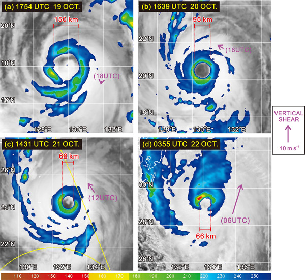
Satellite appearance of Typhoon Lan at the 85 GHz wavelength polarization-corrected temperature (courtesy of the Naval Research Laboratory/Monterey). The imagery is from (a) SSMI at 1754 UTC on 19 October, (b) GCOM-W at 1639 UTC on 20 October, (c) GPM at 1431 UTC on 21 October, and (d) GPM at 0355 UTC on 22 October. A vector on each panel indicates the vertical wind shear derived from the JRA-55 Reanalysis data at the closest hour from observation.

Radius-time plot of the azimuthal-mean infrared cloud-top temperature. Contours of 0°C are highlighted in yellow. Horizontal lines indicate the time of eye soundings (DS-R and DS-V), microwave satellite observations (shown in Fig. 6), and landfall. Purple crosses indicate the period during which this typhoon possessed an annular typhoon structure. A bold broken line indicates the eye radius subjectively estimated using microwave satellite images (Fig. 6).
The detailed three-dimensional structure of the eyewall approximately 3 h after the second flight mission was captured by the Ku-band radar on board the GPM core spacecraft (Fig. 8). This was the only three-dimensional precipitation distribution of Lan observed near the two flight missions. The eye had been masked by upper-level cloud shields (Fig. 8a), while a clear eyewall structure was maintained below that (Figs. 8b, c). The storm center was subjectively identified using the precipitation patterns at the altitudes of 8.0 km and 2.0 km MSL, which are indicated by an open circle and an open square, respectively. The vertical section along the A–A′ line (Fig. 8d) shows that the storm center tilted toward the north-northeast with height, in accordance with the vertical shear direction (indicated in Fig. 8a). The center displacement between the two altitudes was 15–20 km. This shearrelative typhoon tilt is consistent with composite analysis using an airborne radar by Reasor et al. (2013), although the tilt was greater than that in their composite (∼ 3 km between the altitudes of 2 km and 7 km MSL), probably due to the vertical shear magnitude (13.6 m s−1 at 0000 UTC), which was larger than that in their study (0–10 m s−1). In this vertical section, the radius of a precipitation-free region of the eye at 2.0 km MSL was 22 km, and that of the heaviest precipitation core of the eyewall was 42 km. The eye radius identified using microwave imagery (i.e., 33 km, Fig. 6) was approximately in the middle of these radii. The vertical section along the B–B′ line (Fig. 8e) shows that deep eyewall convection developed to the northwest of the center, corresponding to the left side of the shear vector. The development of eyewall convection in the downshear left side is consistent with the results of previous observational studies (Black et al. 2002; Eastin et al. 2005; Reasor et al. 2013).

Horizontal distributions at 0355 UTC on 22 October of (a) the infrared cloud-top temperature observed by Himawari-8 and (b, c) the precipitation rate at 8 km and 2 km MSL observed by the Ku-band precipitation radar on board the GPM core satellite. A cross indicates the interpolated storm center using the JMA best track. A red open circle (square) indicates the storm center subjectively identified from the precipitation rate at 8 (2 km) MSL. A broken circle indicates the 150 km range from the subjectively identified storm center at 8 km. (d, e) The vertical cross sections of the precipitation rate and cloud-top height along A–A′ and B–B′ lines.
In summary, the evolution of Lan was characterized by the formation of an annular structure, followed by an increasing vertical wind-shear effect. We speculate that the uncertainty in the operational intensity estimation on 22 October, as seen in the discrepancy of the best track records, was related to the fact that the eyewall structure was masked by the upper clouds as the shear increased. It is also speculated that the annular eyewall structure began to be affected by moderate vertical shear during the first flight. The speculation motivated us to clarify how the thermodynamic structure in the eye changed with increasing shear. In subsequent sections, we describe these points using dropsonde data.
The shear-induced wavenumber-1 asymmetry was examined using dropsondes deployed on 21 October. Figures 9a–d shows the azimuth–height plots of the system-relative radial velocity (Vr , left panels) and the equivalent potential temperature (θe, right panels) using nine dropsondes (labeled C, D, and H–N) deployed during a circumnavigational flight in the radii between 80 km and 150 km (see Fig. 4a). We consider that all of these dropsondes were deployed just outside the eyewall updrafts because the upward vertical velocities estimated using these dropsondes were at most 1.5 m s−1 in the upper troposphere, and the microwave image on this day (Fig. 6c) indicates the concentration of intense eyewall precipitation within a radius of approximately 60 km. The sounding data were linearly interpolated in the azimuthal direction (top panels), and harmonic analysis was performed at each altitude to compute the wavenumber-1 asymmetric components (middle panels). Nine soundings in a full circle (i.e., mean azimuthal intervals of 40°) are generally within an acceptable range to extract the wavenumber-1 component. The directions relative to the environmental shear vector (Fig. 5b) are indicated in the middle panels of Fig. 9. A hodograph of the wavenumber-1 Vr component is shown in Fig. 9e. This represents the shear-induced flow structure above 4 km MSL: a flow of ∼ 9 m s−1 toward the west-northwest (i.e., downshear-right) above 10 km MSL and that of ∼ 5 m s−1 toward the east-southeast (upshear-left) at about 4 km MSL. This shear-induced wind structure is consistent with that associated with observed (e.g., Black et al. 2002; Reasor et al. 2013) and numerically simulated (e.g., Braun et al. 2006; Cram et al. 2007; Zhang and Rogers 2019) TCs with a moderate vertical shear. In contrast, the directions below 4 km MSL deviate from the shear-induced flow direction: a counterclockwise rotation with decreasing height and the direction at around 1 km MSL corresponding to that of the storm motion5. Since this flow causes a divergence ahead of (convergence behind) the storm motion, this is different from an asymmetry induced by a frictional convergence in the boundary layer (e.g., Shapiro 1983; Corbosiero and Molinari 2003). We consider two possible factors related to the wind shift in the lower troposphere. One is the enhancement of inflow due to the merging of a weak spiral band with the eyewall on the southern side, which can be identified from the cloud distribution (Fig. 2). The other is the acceleration of the storm motion during flight time (dotted line in Fig. 5b), probably related to a change in the environmental flow structure as the storm approached the midlatitude. Although an investigation of the flow structure outside the inner core is beyond the scope of this study, it is noteworthy that the inflow toward the eyewall was enhanced on the southern side (i.e., the left-of-shear semicircle) in the lower troposphere. The shear magnitude between 2 km and 11 km MSL (generally corresponding to the 850–200-hPa layer) was approximately 13.1 m s−1, which was more than twice as strong as the environmental shear (4.8 m s−1, Fig. 5c), while the simulation by Tsujino et al. (2021) represented a comparable strength of vertical shear (∼ 14 m s−1 in Fig. 1c of their paper). We consider the dropsondes to have effectively captured the near-storm vertical shear, which cannot be sufficiently represented in the JRA-55 dataset. The shear-induced asymmetry is also evident in the wavenumber-1 component of the θe (Fig. 9d) in the boundary layer: a warmer peak of ∼ 8 K on the left side of the shear vector. The asymmetric distribution of θe outside the eyewall convection, with a warm anomaly on the left side of the shear vector, is identified in the composite analysis by Zhang et al. (2013) although the focus of their study is the asymmetry inside the eyewall. The boundary-layer inflow with warmer air on the left side of the vertical shear corresponds to the peak rainfall intensity on the southern side of the eyewall, identified in the microwave satellite image (Fig. 6c). The results suggest that the asymmetry of the eyewall convection was already apparent during the first flight. It is necessary to consider the effect of shear in the subsequent analysis of the structure in the inner-core region.

(top) The azimuth-height plots of the (a) radial velocity (Vr) and (b) equivalent potential temperature (θe), observed by nine dropsondes in a radius between 80 km and 150 km from the storm center on 21 October. Trajectories of the dropsondes are shown as bold curves. (middle) The wavenumber-1 components of the (c) Vr and (d) θe . Broken lines indicate the directions relative to the environmental shear vector shown in Fig. 5. (e) Hodograph computed using the wavenumber-1 Vr component. Each black box indicates the altitude. A bold white arrow indicates the vertical wind shear between 2 km and 11 km MSL, and a bold gray arrow indicates the environmental shear vector between 850 hPa and 200 hPa computed using the JRA-55 dataset (shown in Fig. 5), while a thin arrow indicates the storm motion at 0600 UTC.
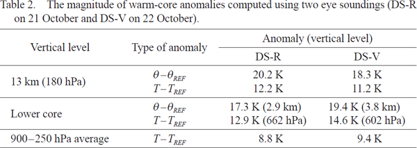
The vertical profiles of two eye soundings, DS-R (DS-V) on the first (second) day, are shown in Fig. 10. The profiles from DS-R were obtained at a radius of 5.5–7.5 km from the storm center (see Fig. 4a). The magnitudes of the radial (Vr) and tangential (Vt) winds relative to the storm center were less than 6 m s−1 in the whole layer, suggesting that the dropsonde fell within a calm region of the circulation center. It is noteworthy that the wind profile near the circulation center was less affected by the vertical shear observed outside the eyewall (Fig. 9). The perturbation potential temperature from the reference sounding, defined as θ–θREF, shows positive values extending from the lower through the upper troposphere, with a local peak of +17.3 K at 2.9 km (∼ 662 hPa) and a maximum of +20.2 K at 13.0 km MSL (180 hPa). With regard to the upper warm anomaly, we checked the height of the peak anomaly using the AMSU perturbation temperature (see Supplemental Fig. S1a), which showed a peak at 150 hPa. This pressure level was approximately 1.1 km above the upper limit of the eye sounding (180 hPa). Hence, it follows that the increasing trend of θ–θREF above 11 km MSL corresponds to the bottom of the upper-tropospheric warm core. This is a rarely observed double warm-core structure; there is a very limited number of cases in which in situ and/or dropsonde observations have been made at such a high altitude above an intense TC (i.e., Hawkins and Imbembo 1976; Schwartz et al. 1996; Stern and Zhang 2016; Rogers et al. 2017). The altitude of the lower core (2.9 km MSL) was lower than that (5–6 km MSL) in previous observations6 (Hawkins and Imbembo 1976; Halverson et al. 2006; Munsell et al. 2018) and numerical simulations (e.g., Stern and Nolan 2012; Kieu et al. 2016; Zhang et al. 2020).

Vertical profiles within the eye of (a, c) the potential temperature θ, the equivalent potential temperature θe, and the saturated equivalent potential temperature θe* and (b, d) system-relative radial and tangential wind components observed by (top) DS-R and (bottom) DS-V. The potential temperature of the reference sounding (θREF) and the perturbation temperature defined as θ–θREF are drawn as a broken line and a solid purple line, respectively. For comparison, the profiles of θ–θREF and θe observed by DS-R in (a) are also drawn in (c) as dotted lines. The altitude of eyewall cloud tops, averaged azimuthally in the radii between 80 km and 120 km, is drawn as a dash-anddotted line.
The eye sounding of DS-V on the next day (bottom of Fig. 10) also shows the double warm-core structure. The peak of the perturbation temperature (θ–θREF) was +19.4 K at 3.8 km MSL. Compared with the eye sounding on the previous day (dotted line), this value increased by 4.7 K at 4.2 km MSL while it decreased by 2.5 K at 11.2 km MSL. This sounding, obtained 17–24 km north of the storm center, shows an increase in wind speed below 5 km MSL. This increase probably reflects a combination of the general increase in wind with decreasing height as the dropsonde moved away from the immediate center and the tilt of the center with height in the sheared environment (Fig. 8d). Nevertheless, this sounding provides evidence that the double warm-core structure was maintained against the strengthening environmental vertical shear (Tsujino et al. 2021). In the AMSU temperature anomaly during the dropsonde observation (Supplemental Fig. S1b), the lower warm core was missing, although slight tilting of the warm-core structure leftward with respect to the wind shear vector with height was identified. The missing lower core was probably due to the attenuation caused by upper-level precipitation and/or the insufficient horizontal resolution (> 45 km) of a microwave sensor to detect it (Stern and Nolan 2012).
The magnitude of the warm-core anomaly is summarized in Table 2. As the definition of a warm anomaly varies among studies (Durden 2013), we performed two types of calculations: the perturbation potential temperature (θ–θREF) at a certain altitude and the perturbation temperature (T–TREF) at a certain pressure level. Regardless of the definition, these values show the warming of the lower core from the first to the second day despite the cooling trend of the upper core. To examine the deep-layer strength of the warm anomaly, a mean value of the perturbation temperature between 900 hPa and 250 hPa (Durden 2013) was also computed. A slight increase in the mean anomaly from 8.8 K to 9.4 K reflects the warming in the lower core and the slight cooling in the upper core (Fig. 10c). It is known that a warm anomaly in the eye results from the adiabatic descent as a response to condensation heating in the eyewall (e.g., Shapiro and Willoughby 1982; Vigh and Schubert 2009). A positive relationship between the warm anomaly and storm intensity was demonstrated in previous observational (e.g., Durden 2013; Doyle et al. 2017) and numerical (Zhang et al. 2015, 2020) studies. We speculate that the continuous eye warming reflected the maintenance of eyewall convection, which is identified from the azimuthal-mean infrared cloud-top temperature (Fig. 7), with cloud tops near or colder than −75°C at radii between 60 km and 150 km in the period between DS-R and DS-V.
In Fig. 10c, the two eye soundings show common characteristics of the θe profile: a lower value (∼ 355 K) at the lower warm core and a higher value (> 365 K) in both the upper troposphere (> 9 km) and the near-surface boundary layer (∼ 1 km MSL). Since θe is conserved in dry adiabatic and irreversible moist adiabatic processes, this difference implies that the lower core had a different origin from the upper core and the boundary layer. Willoughby (1998) hypothesized that the air in the lower core had remained isolated and subsided a few kilometers at most in the eye since the time it was enclosed by eyewall clouds. In our observation, the idea of dry adiabatic descent is supported by an extremely large value of the saturation equivalent potential temperature (θe*) reaching 420 K or higher. The increase in θe* is explained by an exponential increase in the saturation vapor pressure with increasing temperature due to adiabatic compression.
The maximum θe values observed in the upper troposphere and the boundary layer on each day are summarized in Table 3. It is noteworthy that these values are similar, near 380 K, with only small differences. Such a high θe was not observed outside the eyewall (Fig. 9b): the maximum was 363 (373) K at 0.5 (13.0) km MSL. The boundary layer with an extremely high θe value in the eye is known as a reservoir of high-enthalpy air, built through sensible and latent heating from the sea surface (e.g., Dolling and Barnes 2012; Zhang et al. 2013). The connection between the boundary layer and the upper warm core in the eye is described in Sections 6 and 7.

To quantitatively assess the depth of subsidence, saturation-point analysis (Betts 1982) was performed. In subsaturated air, the saturation point is essentially the lifting condensation level determined by expansion of the parcel along a dry adiabat, keeping a constant water vapor mixing ratio, until saturation is reached at pressure PSAT (Willoughby 1998). Thus, the saturation pressure difference from the original pressure (PSAT–P) corresponds to the maximum depth of adiabatic descent. In the case of air entrained from the eyewall, PSAT corresponds to the pressure level of entrainment. For convenience, the saturation point is represented as the altitude (ZSAT), and the saturation height difference (ZSAT–Z) is represented as the difference from the original altitude, under the assumption of hydrostatic balance. Note that this analysis assumes adiabatic processes and does not consider turbulent mixing or radiative cooling. Figure 11 indicates the vertical profiles of the saturation height difference observed by all dropsondes within the eye. On 21 October (Fig. 11a), two profiles near the storm center (P and R) show a saturation point of approximately 2 km at the lower core (∼ 3 km MSL). All soundings on 22 October (Fig. 11b) show similar values at the lower core (∼ 4 km MSL). This result supports the idea that the lower warm core was formed through a dry adiabatic temperature rise with a subsidence depth of ∼ 2 km. If we assume the entrainment of saturated air from the eyewall, the entrainment altitude is estimated to be 5–6.5 km MSL, roughly corresponding to the melting level.
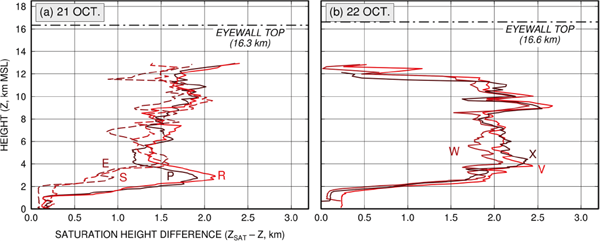
Vertical profiles of the saturation height difference (ZSAT–Z) calculated using all the eye soundings on (a) 21 October and (b) 22 October.
The profiles in Fig. 11 are also marked by the increase in ZSAT–Z in the whole middle troposphere (4–8 km MSL) and the significant decrease above 11.5 km MSL on the second day. They quantitatively support the idea of enhanced subsidence in the eye and strengthened ventilation of the upper warm core on the second day. An interesting point is that the θe at 13 km MSL was almost constant on these days (∼ 379 K, Table 3) despite the strengthened ventilation. The saturation point (ZSAT) at this altitude was approximately 15 km (i.e., ZSAT–Z of ∼ 2 km) on 21 October (Fig. 11a), lower than the mean cloud-top height of the eyewall derived from the satellite product (16.3 km, indicated by a dash-dotted line). In the reference sounding (θREF in Fig. 10), air with a similar θe in the eye was found at a considerably higher altitude (∼ 17 km MSL) than indicated by saturation-point analysis (i.e., 15 km MSL). This implies that the air observed in the upper warm core could not have occurred solely by subsidence from the lower stratosphere. However, this is somewhat contrary to the idea in previous studies (Stern and Zhang 2013b; Ohno and Satoh 2015; Kieu et al. 2016) showing the subsidence (or inflow) from the lower stratosphere. Since turbulent mixing is not considered in the saturation-point analysis, it is possible to hypothesize that the air descending from altitudes above the cloud tops mixed with moist air from the eyewall. Even in this case, since air from the stratosphere contains a very small amount of water vapor, supply of water vapor from the eyewall is necessary to keep the saturation point below the cloud top. The numerical study of Lan by Tsujino et al. (2021) showed that the warming in the upper warm core was partly induced by inward acceleration from the eyewall due to departure from the gradient wind balance. The importance of total temperature advections in warm-core development is also demonstrated by Biswas et al. (2020). These studies led us to speculate that the shear ventilation effect could cause the transport of warm and moist air from the eyewall, which was transported through the eyewall updraft from the boundary layer. The kinematic and thermodynamic structure between the eye and the eyewall are described in the following sections.
To illustrate the radial and vertical structure of the eye and eyewall, dropsondes deployed in the inner core on 21 October were employed for further analysis. Figure 12 shows the descent trajectories for eight dropsondes within a 60-km radius from the storm center, superimposed on visible satellite images. Four sondes (E, P, R, and S) were deployed in the eye with a cloud-top temperature (indicated by contours) higher than 10°C, while two sondes (F and G) were deployed in the eyewall with colder cloud tops on the left side of the environmental shear vector (indicated by an arrow). These dropsondes are used to show the radialvertical structure in the left-of-shear semicircle where the low-level inflow was enhanced (Fig. 9). In addition, two more sondes (Q and T) were deployed in the eyewall on the downshear side.
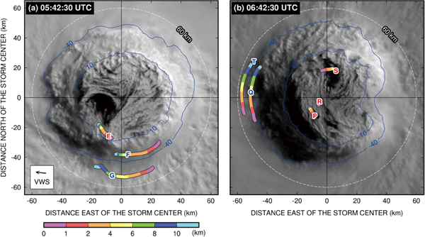
Visible satellite images at (a) 05:42:30 UTC and (b) 06:42:30 UTC on 21 October. Blue solid curves indicate −40°C and 10°C contours of the infrared brightness temperature. The descending trajectories for eight dropsondes relative to the storm center are indicated by color. Letters indicate the position of the dropsondes at the time of each satellite image, except for T, which indicates the drop location 3 min and 20 sec after this time. The vertical wind shear (VWS) vector at 0600 UTC is indicated in panel (a).
It is worth mentioning that Fig. 12 captured cloud features suggesting an eye–eyewall mixing process. The eye was filled by convoluted cloud streets with a relatively large cloud-free region, corresponding to shallow stratocumuli in the aerial photograph (Fig. 1a). Tsukada and Horinouchi (2020) examined the rotation speed of these clouds using a spectral analysis of visible satellite images. They revealed that clouds between 15 km and 25 km radii rotated almost as a rigid body, with a constant angular velocity of ∼ 1.2 × 10⁻³ rad s−1 (i.e., a full orbit in approximately 85 min). They also showed a radial increase in the angular velocity near a 30-km radius, where curved and finger-like cloud features were identified (Fig. 1b). Figure 13a shows the radial profile of the angular velocity (Vt/r, where r is the radius) at 1.0 km MSL, computed using the dropsondes. This profile shows an almost constant value in the radii between 15 km and 30 km, consistent with the results of Tsukada and Horinouchi (2020). The profile also shows the maximum value near a 40-km radius and a decrease in roughly inverse proportion to the distance outside this, implying a radius of maximum tangential wind near 40 km. A distinct radial increase in the angular velocity between dropsondes E and F reflects a barotropically unstable flow field (i.e., Regime 1 of Kossin and Eastin 2001) that is usually observed in intensifying TCs (Rogers et al. 2013a). Mesovortices develop in a barotropically unstable flow across the eye–eyewall interface and cause vigorous turbulent mixing, as reported in previous studies (Kossin et al. 2002; Guimond et al. 2016; Braun et al. 2006). We speculate that a series of curved and finger-like cloud features along the inner eyewall boundary, most pronounced in the eastern and northern sides (i.e., the leeward side of the low-level flow), resulted from tornado-scale vortices and extreme low-level updrafts (Zhu et al. 2014; Stern et al. 2016; Stern and Bryan 2018; Wu et al. 2018). An observational study by Sanger et al. (2014) shows that convective-scale rotating updrafts develop near and just within the radius of maximum tangential winds where the winds are significantly supergradient near the top of the boundary layer. They suggest that the rotating updrafts and supergradient winds in the eyewall are important elements in the spin-up process in the boundary layer (e.g., Smith et al. 2009). Although the importance of supergradient winds in storm intensification is still under debate, an idealized numerical study by Li et al. (2020) shows that the upward advection of the supergradient winds contributes about 10–15 % to the final storm intensity due to the enhanced inner-core air–sea thermodynamic disequilibrium. To briefly examine the dynamically balanced state in the eyewall boundary layer, the gradient wind speeds (Vtgr) were calculated using the regressed radial pressure distribution in a manner similar to that in Sanger et al. (2014). Figure 13b shows the result of cubic polynomial curve fitting to the observed pressure. The curve fitting was judged to be good7 with a coefficient of determination values (R2) of 0.97. The plot of the computed gradient wind speeds as well as observed tangential wind speeds (Vt) in Fig. 13c shows that significant supergradient winds were captured by the eyewall soundings (F and G) in the left-of-shear side, which suggests that the spinup process remained in the eyewall boundary layer, at least on this side, even though the storm had reached steady-state intensity. In the following analyses, we emphasize the kinematic and thermodynamic contrasts between the eye and the eyewall.
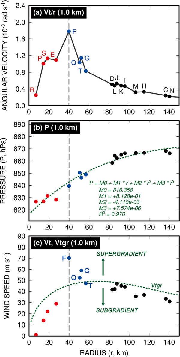
The radial plots of (a) angular velocity (Vt/r), (b) pressure, and (c) tangential wind speed (Vt) at 1.0 km MSL. A broken line indicates the approximate location of the radius of maximum tangential winds. Observations in the eye are plotted in red while those in the eyewall (the surrounding region) are plotted in blue (black). A green dotted curve in (b) shows the cubic polynomial curve fitting to the pressure, and that in (c) shows the gradient wind speed (Vtgr) computed using the cubic polynomial curve of the pressure.
The sounding data were projected onto a single radius–height domain (Fig. 14) with horizontal (vertical) grid spacing of 1.0 (0.1 km). The radial displacement of the dropsondes relative to the storm center during descent is considered in this plot (Fig. 14a). Data were first interpolated onto grid points adjacent to a sounding point using the Cressman (1959) weighting factor within an influence ellipsoid with the horizontal (vertical) radius of 3.0 (0.5) km. Gaps outside the Cressman interpolation were linearly interpolated only in the horizontal direction. In each panel, a bold broken line indicates a 70 % contour of relative humidity (Fig. 14b) as a proxy for the cloud edge, while a hatched area indicates a Vt equal to or greater than 50 m s−1 (Fig. 13f) to highlight the area of maximum wind. The horizontal spacing of the soundings (shown in Fig. 14a) is less than 10 km in the eye, while it is approximately 13 km in the eyewall. Because this resolution is less than that needed to appropriately resolve structures, particularly in the high-gradient region of the eyewall, it is necessary to pay attention to this sampling issue when examining the eyewall structure. For example, in the radial velocity (Vr) distribution (Fig. 14e), a lack of positive radial velocity near a 43-km radius at 6 km MSL, where a contiguous outward-tilting updraft is expected, is probably due to lack of observation.
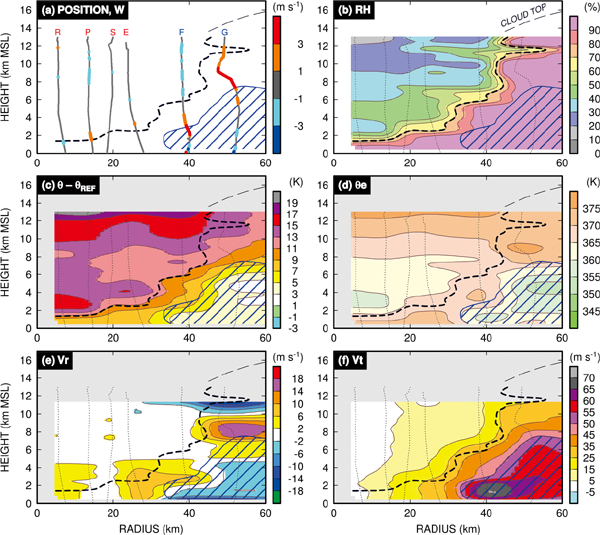
The radius-height plots of (a) the dropsonde position and vertical velocity, (b) relative humidity, (c) potential temperature perturbation, (d) equivalent potential temperature, and system-relative (e) radial and (f) tangential velocities, observed in the eye and the left-of-shear semicircle between 0515 UTC and 0654 UTC on 21 October. A bold broken line indicates the 70 % contour of relative humidity, and a long-dashed line indicates the azimuthally averaged cloud-top height above 13 km MSL. A hatched area indicates the tangential velocity equal to or larger than 50 m s−1.
The 70 % humidity contour sloped outward with increasing height between radii of 30 km and 45 km and roughly connected with satellite-derived cloud tops (a thin long-dashed curve). This sloped structure corresponds to the visual feature in the photograph (Fig. 1a). The outward-sloping shape near the inner eyewall boundary is also identified in the contours of the perturbation potential temperature (θ–θREF, Fig. 14c) and those of the Vt (Fig. 14f), in accordance with the thermal wind relationship. In Fig. 14e, the Vr distribution between dropsondes E and F is marked by a near-surface inflow at a 40-km radius and the prevalence of an outflow inside and above it. This corresponds to the overshoot of the boundary layer inflow into the eye before returning outward to the eyewall updraft, which is consistent with the numerical simulation by Tsujino et al. (2021) and supports the idea of eye–eyewall mixing mentioned above (Fig. 13). The prevalence of the near-surface inflow beyond the 40-km radius is also consistent with the asymmetry of Vr in the lower troposphere (Fig. 9). Figure 14a shows that vertical velocities greater than 3 m s−1 (red dots) were diagnosed in a narrow region between the cloud boundary and high-Vt area, and they corresponded to the eyewall updraft. The location of the eyewall updraft inside the radius of the maximum Vt is consistent with that examined in previous studies of intensifying storms (e.g., Rogers et al. 2013a). This updraft area is generally characterized by a θe exceeding 365 K (Fig. 14d) and an outward radial flow (positive Vr) greater than 2 m s−1 (Fig. 14e), although a discontinuity due to a sampling issue is seen at around 6 km MSL. The coexistence of a high θe with upward motion is highlighted using a scatterplot of the two variables (Fig. 15). This plot was drawn using individual sounding data within a 60-km radius rather than the interpolated data used in Fig. 14. Four eyewall soundings (F, G, Q, and T) show updrafts stronger than 3 m s−1, and two of them (F and G) show updrafts stronger than 5 m s−1, which is close to the magnitude of updrafts treated as convective bursts (> 5.5 m s−1) in previous studies (e.g., Rogers et al. 2013a; Hazelton et al. 2017). The profile of DS-G clearly shows that the eyewall updraft at 9.1 km corresponds to rising air with a θe higher than 370 K. Interestingly, the profile of DS-F shows that the updrafts in the layer between 2 km and 4 km MSL (drawn in orange) possessed a wide range of θe from 363 to 371 K, with a higher value on the upper side. This led us to speculate that the eyewall updrafts had a two-layer structure with different origins of air in the lower troposphere. Eastin et al. (2005) described similar characteristics of buoyant updraft cores that exhibited a higher θe on the inner side of the eyewall. They pointed out that the θe was higher than that observed in the low-level eyewall but equivalent to that observed in the eye boundary layer.
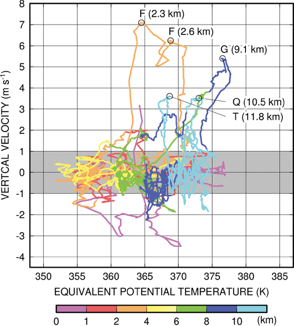
Scatterplot of the equivalent potential temperature versus vertical velocity, using noninterpolated dropsonde data within a 60 km radius from the storm center. Color indicates the altitude of measurement. The peak updrafts observed by dropsondes within the eyewall are highlighted by open circles with a label noting the altitude.
Returning to Fig. 14d, areas of θe higher than 370 K are concentrated in the eye boundary layer, eyewall updraft, and upper warm core. This suggests that a flow of high-θe air from the boundary layer through the eyewall updraft contributed to the development of the upper warm core. However, it should be mentioned again that the 370 K contours of θe were not continuously connected in the eyewall near the altitudes of 3 km and 6 km MSL due to the horizontal sampling issue with this plot. In addition, it is speculated that the distribution in Fig. 14d includes a narrow zone of downdrafts along the eye–eyewall interface (e.g., Stern and Zhang 2013a; Tsujino et al. 2021). This makes it difficult to identify the path of air solely from this distribution. Thus, the flow between the eye and eyewall is diagnosed from the viewpoint of thermodynamics in the next section.
We attempt to trace the flow of high-θe air in the eyewall using a concept based on the parcel method. Since the eye boundary layer was almost saturated (Fig. 14b), rising air parcels originating from the eye should have undergone temperature decreases according to the moist adiabatic lapse rate. In other words, rising air parcels should conserve the pseudo wet-bulb potential temperature (θw) unless it undergoes turbulent mixing or diabatic heating other than condensation. Thus, a layer in which the observed temperature fits to a single moist adiabatic line should represent air originating from the eye boundary layer if upward motion would have coexisted. Three dropsondes (E, F, and G) across the eyewall in the left-of-shear semicircle (Fig. 12a) were employed for this diagnosis because they were released almost in the radial direction within a short period of time (∼ 5.5 min).
Figure 16 shows the skew T-log p diagrams (top panels) and the vertical profiles of wind components (bottom panels). In the eye (Fig. 16a), the boundary layer (< 2.1 km MSL) was almost saturated, and the temperature in this layer almost fits to the pseudo wetbulb potential temperature (θw) of 27.7°C at 1000 hPa (indicated by a solid purple curve) except for the layer closest to the surface. This higher temperature in the lowest level is probably due to sensible and latent heating from the sea surface (e.g., Dolling and Barnes 2012; Zhang et al. 2013). The observed air temperature at the lowest point was 26.7°C, which was slightly colder than the satellite-derived sea surface temperature (27.8°C) averaged before and after the passage of Lan.
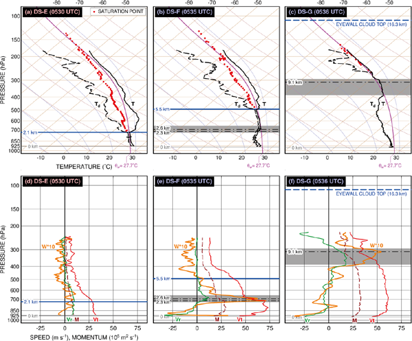
(top) Skew T-log p diagrams and (bottom) the vertical profiles of wind components (Vr, Vt, W) and the absolute angular momentum (M) observed by dropsondes in the eye (DS-E) and eyewall (DS-F and DS-G). The vertical velocities are multiplied by a factor of 10. Layers with updrafts greater than 3 m s−1 are shaded. Horizontal dash-and-dotted lines indicate the altitude with a peak updraft (Fig. 15) while blue solid lines indicate the top of the moist layer with relative humidity greater than 80 %. Red circles in the upper panels show the saturation point of undersaturated layers at every 10 hPa.
The θw profile of the same value is superimposed onto the thermodynamic diagrams in the eyewall (Figs. 16b, c). The temperature profile observed by DS-F almost fits to this θw profile in a layer between 700 hPa and 500 hPa (i.e., 2.5–5.5 km MSL), which partly overlaps with an updraft layer (W > 3 m s−1 at 2.3–2.6 km MSL, shaded). Within this updraft layer, the temperature profile almost fits to the θw profile above 2.6 km MSL while the temperatures below 2.3 km MSL were lower than the θw profile. This implies that the updraft core observed by DS-F had a two-layer structure with warmer air on the upper (inner) side than on the lower (outer) side, as shown in Fig. 15. In the profile of DS-G, the θw profile almost fits to the temperature profile in the saturated updraft layer between 400 hPa and 300 hPa (i.e., 7.1–9.3 km MSL). This profile also shows that the air temperature was slightly higher (lower) than the θw profile in the upper (lower) side of the updraft layer. The constant θw value in the eyewall updraft suggests that saturated air parcels from the eye boundary layer moved upward in the eyewall under an irreversible moist adiabatic process.
Next, the flow structure between the eye and eyewall is examined using the vertical profiles of wind components (Vr, Vt, W) and absolute angular momentum (M ≡ rVt + 0.5 fr2, where r is the radius and f is the Coriolis parameter). The eyewall soundings (Figs. 16e, f) show that updrafts (shaded layers) coincided with positive values of the radial velocities (Vr), implying that the eyewall updrafts sloped outward with increasing height. This feature is similar to the outflow numerically simulated by Hazelton et al. (2017), which flows from the eye to the eyewall, helps mix high-θe air into the eyewall, and aid in the development of convective bursts. The updraft layer is also marked by decreases in both Vt and M with height. The M profile of DS-F decreases from 28.3 × 10⁵ m2 s−1 (at 2.1 km MSL) to 19.7 × 10⁵ m2 s−1 (at 3.1 km MSL), while that in the DS-G profile decreases from 27.1 × 10⁵ m2 s−1 (at 7.4 km MSL) to 17.5 × 10⁵ m2 s−1 (at 9.5 km MSL). The angular momentum greater than 25 × 105 m2 s−1 coexisted with a Vt greater than 50 m s−1, probably resulting from the typical transverse secondary circulation. The significant change in the M in the updraft suggests that the eyewall updraft was composed of two types of air flows with different thermodynamic and kinematic properties. This supports the idea that the higher θe air with a lower M in the upper (inner) part of the updraft originated from the eye boundary layer. The different origins of eyewall updrafts are described not only in previous observations (Eastin et al. 2005), but also in numerical simulations (e.g., Cram et al. 2007; Hazelton et al. 2017).
In the upper troposphere, the profile of DS-G shows a strong inward radial velocity (i.e., negative Vr). This flow is not erroneous because it followed the inward shift of the GPS position (Fig. 12a), and it was observed within inward-projecting anvil clouds near the cloud top, as seen in Fig. 1a. At and around the height of the peak inward radial velocity (230 hPa, 11.3 km MSL), the temperature almost fits to the θw of 27.7°C. Although this inflow layer was not saturated, the saturation points (indicated by red circles) almost fit to this θw profile due to the very small value of the mixing ratio (qv ∼ 0.5 g kg−1). The highest altitude of the saturation points (indicated by red circles) was 12.9 km (180 hPa), which was evidently lower than the highest eyewall cloud tops (16.3 km MSL, corresponding to 107 hPa, indicated by a long-dashed line). Thus, it follows that the inward radial velocities of subsaturated air in the upper troposphere correspond to a flow of high-θe air entrained into the eye, which probably had reached the saturation point via updrafts and turned to descend to this level in a dry adiabatic process. We speculate that this inflow corresponds to the one induced by the departure from a gradient-wind balanced state (Tsujino et al. 2021).
Based on the radius–height sections, saturation-point analysis, and parcel method, we propose a schematic view (Fig. 17) of the thermodynamic and geophysical pathway for high-θe air parcels from the eye boundary layer through the upper warm core. In the radius–height section in the left-of-shear semicircle (right panel), the parcels in the eye boundary layer were mixed with the overshooting boundary layer inflow from the outside, moved upward on the inner side of the eyewall updrafts, and entrained to the upper warm core. This updraft is distinct from that of the transverse secondary circulation on the outer side of the eyewall in terms of the higher θe and lower absolute angular momentum (M). This pathway, indicated by purple and green arrows, can be superimposed onto the skew T-log p diagrams (left panel). Since the high-θe air in the eye boundary layer is almost saturated, the ascending parcels undergo a temperature change according to the moist adiabatic process with a constant wetbulb potential temperature (shown as a purple curve). After reaching the top of the updrafts, they turn to descend with the dry adiabatic temperature rise (shown as a green curve) and eventually form the upper warm core. The temperature profile of the eye sounding (by DS-R, shown as a solid red curve) shows a value similar to that of this dry adiabatic line (θ ∼ 373 K) near 200 hPa. Note that Lan had an asymmetric structure, and the proposed thermodynamic pathway can only be applied in the left-of-shear direction where eyewall convection was active. As seen in the photograph (Fig. 1b), the eyewall cloud features on the opposite (right-of-shear) side were very different, with no inward protrusion of the upper-tropospheric anvil, suggesting weak eyewall updrafts.
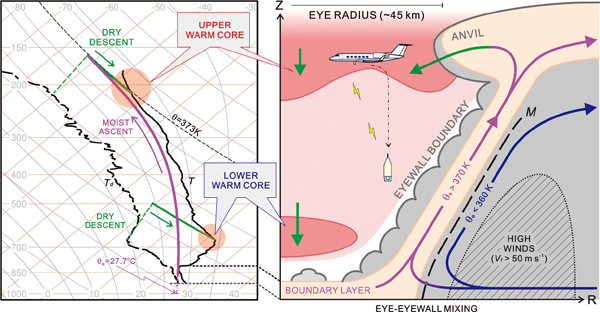
Schematic views of the pathway for air parcels reaching the upper and lower warm cores of annular Typhoon Lan during its mature stage in (a) the skew T-log p diagram and (b) the radius-height section on the left-of-shear semicircle. Purple (green) curves and arrows show moist (dry) adiabatic ascending (descending) flows while a blue arrow shows the transverse secondary circulation. A long-dashed curve shows a contour of the absolute angular momentum. The mixing at the eye–eyewall interface (indicated by a dotted curve) is a speculation based on the radial distribution of the angular velocity (Fig. 13), radial velocity (Fig. 14), and cloud features (Fig. 1).
The lower warm core, on the other hand, differed from the upper core in terms of θe. Saturation-point analysis suggests that the warm-core anomaly can be formed through dry adiabatic subsidence at a depth of up to 2.5 km. Under the assumption of an adiabatic process, this depth suggests that the origin of air in the lower warm core was not the upper troposphere. An entrainment from the eyewall into the eye in the middle troposphere was, however, not captured by dropsondes in the eyewall region (Fig. 14). One possible interpretation is that entrainment occurred in a direction other than the left-of-shear side. The hodograph (Fig. 9a) suggests that the downshear (i.e., western) side was a preferrable region for the entrainment at 4–6 km MSL although the horizontal distribution of dropsondes was not sufficient to diagnose the flow structure in this direction. Another possibility is the isolation of parcels within the eye due to less stirring with the eyewall within an intense TC (Willoughby 1998). A trajectory analysis of simulated TCs by Stern and Zhang (2013b) demonstrated that the degree of stirring between the eye and the eyewall varies greatly with time and height and is a strong function of intensity. In their analysis, stirring is suppressed when a storm reaches sufficient intensity. The simulation of Lan by Tsujino et al. (2021) also demonstrated the reduction of entrainment into the lower warm core in the mature stage. The maintenance of the lower core during the two days of reconnaissance (Fig. 10) during the mature stage supports this idea.
Although dropsonde distribution is insufficient to compute the trajectory of individual air parcels, the numerical study of Typhoon Lan with trajectory analysis by Tsujino et al. (2021) clearly shows that air in the upper warm core originated in the eye boundary layer during the mature stage of this typhoon. In addition, our idea is partly supported by an upper-tropospheric ozone measurement of a mature intense typhoon by Newell et al. (1996). Their study showed a modest decrease in ozone content within the eye, suggesting that the eye in the upper troposphere was filled with air originating from the lower troposphere rather than the lower stratosphere. However, since the maximum altitude of the observation was 13 km MSL, it is not known whether the air descended from the stratosphere at higher altitudes.
Our idea can be applied to estimating the maximum potential strength of the upper warm core if turbulent mixing in eyewall updrafts and a downward transport from the lower stratosphere can be ignored. Assuming an ideal situation, in which all of the air in the upper warm core originates from the eye boundary layer that is saturated, the temperature of the warm core at the level of inflow from the eyewall can be estimated based on the sea surface temperature. In the present case, using the sea surface temperature (27.8°C), the sea-level pressure near the eye–eyewall intersection (928.3 hPa, observed by DS-E), and the associated moist adiabatic line of 303.3 K, the warm-core temperature can be estimated as −42.7°C at 165 hPa (corresponding to a flight level)8. Since the flight-level air temperature measured by a probe mounted on the aircraft body was approximately −50°C in the eye (not shown), the difference of 7.3°C would correspond to the cooling effect of ventilation caused by the environmental wind shear and/or turbulent mixing on the eye warming. If the warm-core temperature is higher than the estimated one, it could be used to diagnose other processes, such as a subsidence from the lower stratosphere. The advantage of this method is that it does not require a reference profile, as compared to using the perturbation temperature.
In this paper, we described the double warm-core structure of Typhoon Lan (2017) as observed through upper-tropospheric flight missions on 21–22 October. This T-PARCII reconnaissance is the first case of a Japanese research group observing the inner core of a typhoon using dropsondes. During the flights, this typhoon achieved a steady state, with an observed minimum central pressure of 926.2 hPa although the environmental wind shear strengthened. Based on satellite images and reanalysis data, this typhoon was characterized by an annular eyewall structure, involving a large eye (∼ 90 km in diameter) that persisted under the strengthened influence of environmental vertical shear. The results of our analysis are summarized below.
These results led us to hypothesize that the vertical transport of high, moist enthalpy air from the eye boundary layer through the eyewall updrafts contributed to the continuous eye warming against a ventilation effect by the strengthening environmental vertical wind shear. This idea is supported by the trajectory analysis using a numerical simulation of this typhoon in the stages from intensifying to mature (Tsujino et al. 2021). We consider the pathway of high-θe air to be important because the warm anomaly in the eye is necessary to maintain a warm-core vortex structure. Although the importance of high, moist enthalpy air for strengthening buoyant eyewall updrafts was pointed out in a previous observational study (Eastin et al. 2005), the present study captured the pathway from the boundary layer to the upper warm core using dropsondes deployed from the upper troposphere. Although the mass of high-θe air in the eye reservoir is considerably smaller than the total mass in the eyewall (Bryan and Rotunno 2009; Zhou et al. 2020), it would not be so small compared with that in the upper warm core. In a rough estimation of mass using the radius–height plot (Fig. 14d), a reservoir (density of 1.0 kg m−3) with a radius of 30 km and a depth of 1 km is equivalent to an upper core (density of 0.3 kg m−3) with a radius of 50 km and a depth of 1.2 km.
Our study demonstrates the significance of eye-penetrating upper-tropospheric reconnaissance to understand thermodynamic processes related to typhoon intensity in the present situation where accurate measurements of both humidity and temperature for calculating θe and saturation-point analysis can only be made with dropsonde-type expendables. Since the altitude of ∼ 13.8 km MSL is almost the upper limit for civil aircraft flight, it is difficult to directly observe the peak temperature anomaly above this altitude. Nevertheless, we could demonstrate that dropsondes deployed from this altitude are useful to capture the warm anomaly in a deep layer (i.e., 900–250 hPa) of the eye.
Another noteworthy point is that the eye-penetration flights could be achieved using a civil jet aircraft, which is usually used for synoptic surveillance flights (e.g., Wu et al. 2007; Aberson and Franklin 1999; Rogers et al. 2013b) and not for eyewall penetration in a TC except in limited cases (e.g., Black et al. 2000). The idea of eyewall penetration within the upper troposphere was proposed about 40 years ago by Gray (1979). He argued that, in the upper troposphere, winds are significantly weaker, and turbulence is generally less intense if echoes can be avoided using aviation weather radar. This was the case in Typhoon Lan (2017), as dropsondes revealed that the wind speed was less than 40 m s−1 above 11 km MSL (Fig. 14f), and there were some portions of the eyewall with weak precipitation (not shown). Our flights were the first attempt to implement Gray's proposal in the WNP. However, two concerns remain with regard to upper-tropospheric reconnaissance. One is the risk of stalling in the eye. The abrupt temperature increase in the warm core causes an increase in the stall speed and increases the risk of stalling. Rogers et al. (2002) pointed out a problem with the cruising speed of the NOAA G-IV jet aircraft, which is close to the stall threshold during the deployment of dropsondes. The reason is that the cruise speed must be as slow as possible to launch a dropsonde without damaging its parachute. We considered this problem to be minor in our flights because the cruise speed during eyewall penetration was in the range of 200–240 m s−1 (i.e., Mach 0.67–0.78), which was close to the maximum speed (Mach 0.85) and had a sufficient margin above the stall speed (Mach ∼ 0.45, corresponding to ∼ 140 m s−1 at ∼ 14 km MSL)9. This safe margin is due to the ability of the iMDS-17 dropsonde to withstand release from a high-speed flight without a parachute.
Another concern is the risk of turbulence due to eyewall updrafts and/or convectively induced gravity waves in the upper troposphere. Previous studies documented signals of gravity waves radiating from TCs (Sato 1993; Nolan and Zhang 2017). Although we fortunately succeeded in reconnaissance without meeting any severe turbulence, there is no guarantee that an aircraft will not meet severe turbulence in a typhoon. Even though convective updrafts with intense precipitation can be avoided using the nose radar system, it is difficult to avoid the clear-air turbulence associated with convectively induced gravity waves and/or deep subsidence. In fact, previous studies reported upper-tropospheric temperature perturbation in the vicinity of deep convective clouds (Holland et al. 1984; Foley 1998; Rogers et al. 2002), possibly associated with gravity waves, subsidence, or instrument error. It is worth investigating and predicting the occurrence of upper-tropospheric disturbances (such as gravity waves from convective bursts) to avoid severe turbulence during reconnaissance. This will be essential to the resurgence of typhoon reconnaissance in the WNP.
The data analysis files are available in J-STAGE Data. https://doi.org/10.34474/data.jmsj.16759906.
Figure S1: Zonal-vertical cross sections of the temperature anomaly derived from AMSU-A data (a) along 23.29°N at 0925 UTC on 21 October and (b) along 28.17°N at 0105 UTC on 22 October. Contours are drawn every 0.5°C above the storm environmental temperature. (Figure courtesy of the AMSU homepage of the Cooperative Institute for Meteorological Satellite Studies, University of Wisconsin-Madison, https://tropic.ssec.wisc.edu/real-time/amsu/.)
The authors express their gratitude to Diamond Air Service Inc. for their support of reconnaissance flights, especially to pilots Dairo Kageyama and Yukinobu Kaneko and flight engineer Hisaaki Kato for their flexibility in flight-route determination inside the typhoon. We are grateful to Dr. Satoki Tsujino for valuable discussions on the development of Typhoon Lan. We also thank three anonymous reviewers for their constructive criticism and helpful comments. This work was supported by JSPS KAKENHI (Grant Numbers JP16H06311, JP16H04053, JP19K03973, and JP21H04992) and University of the Ryukyus Research Project Promotion Grant (Strategic Research Grant 18SP01302). Himawari-8 rapid-scan imagery was provided by the Science Cloud of the National Institute of Information and Communications Technology (https://sc-web.nict.go.jp/SCindex.html). Himawari-8 cloud-top height data were obtained from a data server of the Meteorological Research Consortium (https://www.mri-jma.go.jp/Project/cons/). The 89 GHz polarization-corrected temperature (PCT) imagery was obtained from the Naval Research Laboratory Monterey Tropical Cyclone webpage (https://www.nrlmry.navy.mil/TC.html). The NOAA OISST dataset was downloaded from https://www.ncdc.noaa.gov/oisst. The GPM Ku-radar dataset (Level-2A product) was obtained from the Tropical Cyclone Database of the Earth Observation Research Center (EORC), Japan Aerospace Exploration Agency (JAXA) (https://sharaku.eorc.jaxa.jp/TYP_DB/.) Upper-air soundings at Naze and Minamidaitōjima were provided by the JMA.
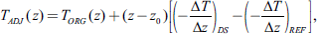
Before the reconnaissance of Typhoon Lan, we deployed dropsondes over the Sea of Japan on 27 July 2017, in a test flight under fine weather conditions with scatted nonprecipitating cirrus clouds (Fig. A1). Based on a comparison with Meisei RS-11G radiosondes launched from Wajima (indicated by a red cross), 100–200 km away from the dropsondes, we recognized that the temperature measured by a dropsonde possesses a positive bias within 125 s after release from the aircraft. The temperature profiles in Fig. A1a show a warm bias of dropsondes from radiosondes above 10 km MSL, causing a decrease in the temperature lapse rate of 1.4 K km−1. Note that the radiosonde profiles (green lines) include measurements during not only ascent, but also descent, suggesting that the warm bias is unique to dropsonde profiles (black lines). Although the cause of this bias has not been elucidated, one potential factor is the influence of radiant heat from the dropsonde body, which is made of expanded polystyrene foam. Since each dropsonde is ejected from the aircraft cabin with an air temperature of ∼ 23°C (indicated by a red star), it seems to take time for the body to cool to the outside temperature. Figure A2 shows the temperature profiles measured by dropsondes in Typhoon Lan and those measured by radiosondes at the JMA 47945 site. In the original profiles (Fig. A2a), the temperature measured by DS-B and DS-A (deployed in the radii of 193–258 km from the storm center; see Fig. 4a) shows a warm bias of up to several degrees from the radiosondes (shown as green lines) above 11 km MSL. Because this bias may negatively affect analysis of the warm-core strength, the temperature bias was corrected using the following equation:
 |

(a) Vertical profiles of temperature measured by radiosondes (green line) and doropsondes (black line) during a test flight over the Sea of Japan on 27 July 2017. Bold-dotted green (black) lines indicate the mean temperature lapse rate between 10 km and 12 km MSL, computed using radiosondes (dropsondes). A red star indicates the mean temperature in the aircraft cabin, measured by dropsondes. (b) The release points of radiosondes and dropsondes, with a four-digit number indicating the time of release, superimposed on a Himawari-8 infrared image on 0340 UTC. The color table is the same as that in Fig. 2.

Vertical profiles of the (a) original and (b) corrected temperature, observed at JMA 47945 (green), in the surrounding area (black), in the eyewall (blue), and in the eye (red) during the flight on 21 October 2017. Green (red) dotted lines indicate the mean lapse rate of the environmental (eye) soundings between 10 km and 12 km MSL.
The vertical velocity was calculated based on the fall rate of dropsondes. Figure A3 shows the relationship between the dropsonde fall rate and air density. It is known that the square of the fall speed of an object (VF2) is generally inversely proportional to the air density (ρ). We performed regression analysis using dropsondes deployed during the test flight on 27 July 2017 (Fig. A1) and obtained the relationship VF = −[148.62/(ρ − 0.014)]0.5. The regression curve shows a fall velocity of −22.6 m s−1 near 200 hPa (ρ of 0.3 kg m−3) and −11.7 m s−1 near the surface (ρ of 1.1 kg m−3). The fall rates are generally equivalent to that of the Vaisala RD93 GPS dropsonde (Fig. 2 of Hock and Franklin 1999) whereas the iMDS-17 dropsonde has no parachute. In the analyses, the vertical air velocity (w) was represented as the deviation of the observed fall velocity from the regressed one. Since the standard deviation was 0.88 m s−1, fall velocities with a deviation greater than 1 m s−1 (indicated in color in Fig. B1) were employed in the analyses (Figs. 14–16).

Relationship between the fall velocity of dropsondes and the air density using dropsondes deployed on 21 October 2017. A regression curve, obtained from dropsondes during a test flight on 27 July 2017, is shown as a bold line. The range of ±3 m s−1 from the regression is indicated by broken lines. Fall velocities with a deviation of more than 1 m s−1 from the regression are colored.
In analyzing the warm core, it is important to choose the reference profile carefully, because the strength of the warm core is sensitive to the shape of the reference profile (Durden 2013; Stern and Zhang 2016). The mean temperature profile of soundings listed in Table 1, obtained at a distance between 270 km and 800 km from the storm center, is employed as an environmental reference in this study. This profile is drawn as a blue curve in Fig. C1a and compared with an azimuthally averaged temperature profile 550–600 km from the storm center, calculated using the JRA-55 Reanalysis dataset and shown as a dashed curve. The two profiles are almost identical, with discrepancies of, at most, 1.1 K at 8.5 km MSL. Figure C1b shows the radius–height distribution of the difference in temperature of the JRA-55 azimuthal mean profiles from the reference profile. This distribution shows that closer soundings are warmer than farther ones, as discussed by Durden (2013) and Stern and Zhang (2016). At an altitude of 8 km MSL, the difference ranges from +1 K near 300 km to −2 K near 750 km. We consider that this ∼ 3 K of uncertainty is small compared to the perturbation temperature of the warm cores (shown in Table 2) using the eye soundings (red curves in Fig. C1a) and does not have a large influence on the analysis of the warm-core structure. This figure also shows the mean temperature profile of the Atlantic hurricane season proposed by Jordan (1958) and that of moist tropical airmass periods proposed by Dunion (2011). These profiles have a colder temperature than the reference profiles. For example, the Jordan profile is 7.8 K colder than the environmental profile at 200 hPa (∼ 12.4 km MSL). This indicates a warmer local environment of a TC compared to the mean environment of the tropics. For reference, using the Dunion profile, the perturbation potential temperature (θ–θREF) of the upper (lower) warm core on 21 October (shown in Table 2) was estimated to be 29.4 (20.5) K at an altitude of 13.0 (2.9) km MSL.
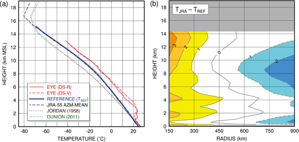
(a) Vertical temperature profiles of the eye soundings (red), the environmental reference sounding (TREF, blue), the azimuthal mean sounding 550–600 km from the storm center, calculated using the JRA-55 Reanalysis dataset (dashed), Jordan's (1958) hurricane season (brown dotted), and Dunion's (2011) moist tropical (green dotted). (b) Radius-height plot of the difference in temperature between the azimuthal mean profiles calculated using the JRA-55 Reanalysis dataset (TJRA) and the reference profile (TREF). Contour interval is 1 K.
The data analysis files are available in J-STAGE Data. https://doi.org/10.34474/data.jmsj.16759906
1An original flight plan to circumnavigate outside the eyewall was modified to penetrate the eyewall after discussion among the first author and the pilots based on aviation weather radar displaying weak precipitation echoes of the eyewall at the flight level.
2Dropsonde O was excluded from analysis due to signal loss in the eyewall.
3The small number of sondes on the second day is because the total number of prepared sondes was 26, and 21 were consumed on the previous day. Originally, the purpose of the second flight was to acquire a water vapor profile in the outer region using a different type of sensor. However, because the typhoon translation speed increased more than expected and the storm center approached the proposed flight track, the mission was changed to a penetration flight.
4It is unclear whether the dropsonde data were used by JTWC for their best track estimates.
5We confirmed that the similar flow structure outside the eyewall was represented in the numerical simulation of Tsujino et al. (2021), although the radial wind distribution near the surface is not shown in their paper.
6An exception is Tropical Storm Humberto (2001), which had a warm-core maximum at an altitude of 2 km (Dolling and Barnes 2012), although that was a much weaker storm than the one analyzed in this study.
7We confirmed that the result changes little if a quartic (quintic) polynomial curve is used, with an R2 of 0.974 (0.978). The choice of curve fitting causes a small range of gradient winds between 40.2 and 47.1 m s−1 at a 40-km radius, as compared with the observed tangential wind speeds of 70.2 m s−1 by DS-F and 58.8 m s−1 by DS-G.
8The surface air temperature is generally a degree or two less than the SST. If the air temperature is assumed to be 26.8 (25.8°C), the warm-core temperature is estimated to be −46.1 (−49.5°C), which is closer to the flight-level air temperature.
9The increase in stall speed due to the 20-K temperature increase is ∼ 6 m s−1.