Materials and methods
1. Statistical methods
1.1. Estimation of the proportion of resistance alleles
Here we discuss how to estimate the proportion of resistance alleles from a given proportion of DNA observed from dead specimens with degraded DNA in the field. The probability distribution of the observed values has three components: (1) the distribution of the numbers of resistant alleles captured by the traps, (2) the distribution of the amount of DNA in an allele, and (3) the distribution of the proportion of resistance DNA for a given number of captured alleles. We will formulate these three distributions consecutively and then combine them to produce the full probability distribution, which can be utilized to estimate the proportion of resistance alleles in the field.
1.1.1. Number of resistant alleles in a trap
We first derive the distribution of the numbers of resistant alleles captured by the traps. Let p be the proportion of the resistant alleles in the field, m the number of resistant alleles in a sample obtained by a trap, and n the total number of the alleles in the sample. The number of susceptible alleles in a sample is given by n−m. We assume that the alleles are mixed well by random mating of the individuals. The distribution of the numbers of captured resistant alleles is given by a binomial distribution with the parameters n and p:
 | (1) |
We use an approximation to describe the probability density function of the amount of measurable DNA per allele in a trapped individual. Let y be the amount of measurable DNA per allele, T the total duration of trapping, and t the time from trapping to collection of an individual. We can use a uniform distribution of the range from 0 to T for the time from trapping to the collection of individuals (t) if we ignore the decrease in attracting ability of a trap (e.g., depletion of pheromone lures or saturation of sticky sheets) and if no information about the phenology of the insects is available. We can assume that individuals enter the trap at random in such situations. We denote the uniform distribution by U(t|0, T). Trapped individuals soon die in the trap, and then DNA degradation (fragmentation) begins because of remnant endogenous DNase activity and ultraviolet solar radiation.10) Exponential decay can generally be assumed for DNA as well as for other materials.16,17) Therefore, the amount of measurable DNA after duration t is given by a exp(−λt), where λ is the rate of decay and a is the initial amount of DNA. The duration of decay, t, follows the uniform distribution U(t|0, T); hence, we obtain the probability density function of the amount of DNA by transforming U(t|0, T) by the function a exp(−λt). Therefore, the probability density function of the amount of DNA (denoted by y) for a given set of λ and T is given by the reciprocal distribution18)
 | (2) |
This equation indicates that the probability density of the amount of DNA (y) falls sharply to zero when y exceeds its maximum quantity a. A schematic example of the probability density is shown in the hatched area of Fig. 1.
The quantity of a in Eq. 2, which indicates the initial amount of DNA before the beginning of decay, will vary between individuals due to the variability in body size.19) Hence, the actual probability density distribution of DNA will be given by a mixture distribution of Eq. 2, i.e., a mixture reciprocal distribution, where the initial amount of DNA (a) varies between individuals. We do not know the distribution of the initial amount of DNA, but the mixture reciprocal distribution will be generally given by a distribution smoothly decreasing toward the right. An example of a mixture reciprocal distribution is shown in the histogram in Fig. 1. This example was generated in a simulated calculation by assuming that the initial amount of DNA follows a lognormal distribution, but the basic form of mixture reciprocal distribution will not largely depend on the underlying distributions of the initial amount of DNA.
We use another class of distribution, a gamma distribution, for approximately describing the mixture reciprocal distribution of the amount of DNA:
 | (3) |
where Γ(∙) indicates a gamma function. The parameters k and θ are the shape and scale parameters of the gamma distribution, respectively. The mean and variance are given by kθ and kθ2, respectively. The quantity of 1/k is equivalent to the coefficient of variation (CV) for the distribution. The validity of this approximation will be shown using the actual field data in a later section. Note that if the trapping duration T is large compared to the mean life-time of DNA (1/λ), i.e., if the quantity of λT is sufficiently large, Eq. 2 becomes identical to Eq. 3 with k=1/(λT) and θ=(λT)2, even if no variability exists in the initial amount of DNA.
1.1.3. Proportion of resistance DNA for a given number of alleles
We next calculate the probability of obtaining a certain proportion of the resistance DNA for a given set of numbers of resistant alleles (m) and the total number of alleles in the sample (n). Let r be the observed proportion of resistance DNA. The amount of resistance DNA in a trap is given by the sum of the DNA of m alleles. The amount of DNA in an allele is approximately given as a gamma variable with the shape parameter k and the scale parameter θ, as discussed above (Eq. 3). We further assume that the distribution of the amount of DNA in an allele is approximately independent although it is not exactly true for diploid insects. Then, the total amount of resistance DNA follows a gamma distribution with the shape parameter km and the scale parameter θ because of the reproducible property of the gamma distribution. Similarly, the total amount of the susceptible DNA in a trap follows a gamma distribution with the shape parameter k(n−m) and the scale parameter θ. Consequently, the distribution of the proportion of resistance DNA, which is denoted by r, is given by a beta distribution with the parameters km and k(n−m) due to the relationship between a gamma distribution and a beta distribution.20) We denote the distribution Beta(r|km, k(n−m)) as follows:
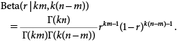 | (4) |
Finally, we calculate the probability of observing the proportion of resistance DNA (r) for a given total number of alleles in the sample (n). The number of resistant alleles (m) among the total alleles in the sample (n) follows a binomial distribution given by Eq. 1. The proportion of the resistance DNA for a given set of m and n follows a beta distribution given by Eq. 4. Hence, we can calculate the probability of observing the proportion (r) for a given number of the total alleles (n) by the convolution of the binomial distribution and the beta distribution for m=1, 2, …, n−1, if the proportion falls within a range of 0<r<1. The proportion becomes r=0 if and only if m=0. The proportion becomes r=1 if and only if m=n. Thus, the probability h(r|n, k, p), in which the obtained proportion of resistance DNA in a trap is r, is given by a set of discrete and continuous distributions:
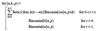 | (5) |
If we calculate the proportion of resistance (r) for each bulk sample, we can estimate the proportion of the resistant alleles (p) as well as the parameter k of the gamma distribution by finding a set of p and k that maximizes the sum of loge(h(r|n, k, p)) given by Eq. 5. A computer program for the estimation of parameter p and its approximate confidence intervals using the R language21) is provided in Electronic Supplementary Material 1 (ESM1). The approximate confidence intervals are calculated using the inverse of the Hessian matrix evaluated at the last iteration of the program.
1.2. Example of estimation using the R function
The proportion of resistant individuals can be estimated by using the R function Resist_est() that is based on the theory described above. The R function is given in ESM1. All ESMs are available on the journal site and on the following site: ‹http://cse.naro.affrc.go.jp/yamamura/Resistance_estimation_from_bulk.html›. We test the function using data generated by simulations. We use the binomial distribution with the proportion of resistant individuals p=0.1 (Eq. 1) and the gamma distribution with the parameter k=1 (Eq. 3).
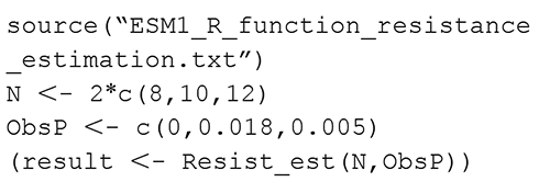
Let us first consider a case where the numbers of captured individuals in three traps are 8, 10, and 12 and the corresponding proportions of resistance DNA are 0, 0.018, and 0.005. The numbers of alleles are 2×(8, 10, 12) for a diploid species. The text file ESM1_R_function_resistance_estimation.txt, which contains the R function, should be placed in the working directory of R software. Then we can perform the estimation as follows: We first use the source function to enable the function. Then we create two vectors named N and ObsP; the N vector contains the number of individuals in each trap, and the ObsP vector contains the quantity of the observed proportion of resistance DNA. The vectors are passed to the R function Resist_est().
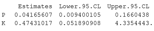
The output is as follows:
The maximum likelihood estimate of the proportion of resistance is p̂=0.042. It should be noted that the estimate is larger than any of the three observations (0, 0.018, and 0.005). The 95% confidence interval is from 0.009 to 0.166. The estimate of the shape parameter of the gamma distribution is k̂=0.474. If we know a reliable estimate of parameter k beforehand from other sources of data, we can use the k-value by adding an optional statement. For example, if we know beforehand that k=1.00, we can use the following script by adding option K=1, although the value of k seems not to largely influence the estimate of p in this case.
The output is as follows:
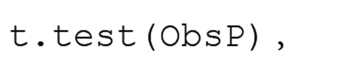
The confidence interval of the proportion of resistance alleles may be biased if we use the classical method, which is based on the assumption of normal errors. For example, if we use the t.test() function of R by specifying
then the results are as follows:
The lower limit of confidence intervals becomes negative (−0.015), and we cannot show the lower limit of the proportion of resistance.
We next use the data for a single trap, where the number of captured individuals is 8 and the observed proportion of resistance DNA is 0.052. The number of alleles is 16 for a diploid species. Hence, we use the following script:
The output is as follows:
The estimate of the proportion of resistance is p̂=0.062. The 95% confidence interval is from 0.009 to 0.335. If we know beforehand that k=1.00, for example, we can add an option K=1. The output is as follows:
The estimate of the proportion of resistance seems to be improved by using this option. Note that the t.test() function cannot yield an estimate of the confidence interval in this case because we have only one observation for the proportion of resistance DNA.
We next use the data for three traps, where the numbers of captured individuals are 4, 2, and 2 and the observed proportion of resistance DNA is 0, 0, and 0, respectively. The numbers of alleles are 8, 4, and 4 for diploid species. No resistance genes are detected in this case; hence, the function yields the simple binomial estimate as follows:
The estimate of the proportion of resistance is p̂=0, and the 95% confidence interval is from 0 to 0.206.
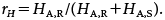
1.3. Calculation of the proportion of resistance DNA from the output of a Sanger sequencer
We next discuss the procedure to calculate the proportion of the resistance DNA (r) from the output of a Sanger sequencer. The DNA sequencer reports the peak height of the fluorescence detector corresponding to each base of the DNA. We denote the peak heights of the critical base of the resistant type (R) and the susceptible type (S) as HR and HS, respectively. The sequencer is designed for qualitative analysis to determine the sequence of DNA; it is not designed for quantitative analysis. Consequently, the peak height does not necessarily indicate the amount of DNA. Therefore, considerable bias may arise if we directly correspond the peak height to the amount of DNA. A proper transformation of the peak height is required to obtain an appropriate quantity of the proportion of resistance DNA (r).
Let xR and xS be the DNA amount of the resistant and susceptible types, respectively. Our current purpose is to calculate the ratio, r=xR/(xR+xS), from the observed peak heights, HR and HS. In the procedure of qualitative detection of materials, the signal for detection should be clearly expressed as a binary form, such as 0 or 1. The signals should increase rapidly with increasing amount of material, while the signals should plateau if the amount of material is sufficiently large. If we want to utilize the qualitative output as a quantitative output, we should take account of the saturation characteristics of the signals. We use the following empirical form of the saturation curve, which is sufficiently flexible:
 | (6) |
 | (7) |
where HMax is a constant that indicates the plateau of the strength of the signals; aR and aS indicate the sensitivity of the signals to the DNA amount of the resistant and susceptible types (xR and xS), respectively; and b determines the form of the saturation curve. This form of saturation-curve has frequently been used empirically. For example, Kono and Sugino22) used it to describe the proportion of rice stems damaged by the rice stem borer, Chilo suppressalis (Walker) (Lepidoptera: Crambidae). Uhlig et al.23) also used it for the detection probability in PCR assays.
Let HA,R and HA,S be the adjusted peak heights for the resistant and susceptible DNA, respectively, which are defined by the following equations:
 | (8) |
 | (9) |
By combining Eqs. 6–9, we obtain the following relation:
 | (10) |
where d is given by d=bloge(aR/aS).
The true proportion of resistance DNA is defined by r=xR/(xR+xS). Hence, the formula inside the bracket on the right side of Eq. 10 is identical to logit(r), that is, loge(r/(1−r)). Similarly, we define the adjusted proportion of the resistant peak height by
 | (11) |
Then the left side of Eq. 10 is identical to logit(rH), that is, loge(rH/(1−rH)). Thus, Eq. 10 is simply written as
 | (12) |
The intercept parameter d is defined by d=bloge(aR/aS), where the parameters aR and aS indicate the sensitivity of signals to the amount of resistant and susceptible DNA types (xR and xS), respectively, as defined above. The sensitivity may fluctuate depending on the conditions of the samples and DNA-sequencing instruments. However, the ratio of sensitivity, aR/aS, should be nearly constant for each (detector) instrument; hence, we can assume that d is a constant in the following analysis.
A nonlinear least squares method is used to estimate the parameters b, d, and HMax in Eq. 12. The peak height is influenced by various factors in a multiplicative manner. Consequently, the error concerning each factor also influences the peak height in a multiplicative manner. If we use a logarithmic scale, the error influences the logarithmic height in an additive manner. Therefore, the logarithmic height will follow a normal distribution with a common variance because of the central limit theorem. Consequently, it is appropriate to apply a nonlinear least squares method to logit(rH) when estimating the parameters of Eq. 12.
A potential problem may arise in the process of estimation in that the peak height (HR or HS) may exceed the quantity of HMax if the peak height is very high. The estimation procedure fails in such cases; hence, the peak height exceeding the quantity of HMax should be replaced by HMax(1−∆) for the convenience of estimation, where ∆ is a small quantity for adjustment. Therefore, we have four unknown parameters: b, d, HMax, and ∆. We can calculate the proportion of the resistance DNA by using the estimated parameters as follows:
 | (13) |
where the peak height (HR or HS) is replaced by ĤMax(1−∆̂) when the peak height is greater than ĤMax. An example of the estimation is provided in an Excel spread sheet in ESM2. The detailed procedure for calculating r is provided in ESM3.
2. Laboratory methods
We demonstrate the validity of our method by using the data for the diamondback moth, P. xylostella, which is a major pest of cruciferous vegetables (ESM2). A single nucleotide mutation of the ryanodine receptor gene (RyR) causes the amino acid mutation from glycine to glutamate at amino acid position 4946 (G4946E), which is responsible for resistance to diamide pesticides such as flubendiamide and chlorantraniliprole.24,25) On September 6–26, 2015, one of the authors (Shoji Sonoda) collected adult males of P. xylostella in the cabbage field of Kagawa Prefectural Agricultural Experiment Station (in Ayagawa: 34°13′54″N, 133°56′08″E) (hereafter referred to as the Kagawa population) using sticky traps equipped with pheromone lures (Sumitomo Chemical Co., Ltd., Osaka, Japan). We extracted DNA individually from the collected insects, time of capture varying from one to five days after installation of the traps. Genotyping for the G4946E mutation was conducted using the individually extracted DNA according to the method reported previously.25) In all, 47 susceptible homozygotes (SS individuals having the nucleotide G) and 48 resistant homozygotes (RR having A) were obtained and used for the subsequent analysis.
PCR amplification of partial RyR was conducted using primers 5′-tgtaaaacgacggccagtagactggcgctaccaagtgt-3′ and 5′-cccgttatgcgtgacagact-3′. In the former primer, the M13-21 primer sequence was included in the 5′ end, as underlined. Quick Taq HS DyeMix (Toyobo Co., Ltd., Osaka, Japan) was used for the PCR amplification. The PCR conditions were 1 cycle of 2 min at 98°C, 32 cycles of 10 sec at 98°C, 15 sec at 58°C, and 15 sec at 68°C, finishing with the final extension of 68°C for 5 min. Amplified DNA fragments were sequenced directly using the M13–21 primer. The nucleotide sequencing was conducted using a dye terminator cycle sequencing kit (Applied Biosystems, Carlsbad, CA, USA) and a DNA sequencer (3130xl, Applied Biosystems). The peak heights of nucleotides corresponding to G4946E were measured from the sequence chromatogram using software (PowerPoint 2016; Microsoft Japan, Tokyo, Japan).
During the process of capillary electrophoresis conducted in a Sanger sequencer, the signal intensities of fluorescence detectors basically correspond to the amounts of the terminal bases, i.e., adenine (A), cytosine (C), guanine (G), and thymine (T), in the hybrid DNA solution. Although the DNA solution contains up to four types of a single-base polymorphism (A, C, G, and T), we discuss only two genotypes, the resistant type R and the susceptible type S, since the frequencies of the other two were negligibly low.
Results
1. Estimation of the calibration parameters (first experiment)
In this experiment, we estimated the parameters of Eq. 13 to calculate the proportion of the resistance DNA (r). We generated artificial solution samples of DNA in which the proportions of resistance DNA were set exactly at predetermined quantities. We first created genuine DNA solutions for the RR and the SS types separately. We mixed a sufficient number of individuals to create the DNA solutions in which the heterogeneity in the amount of DNA among individuals disappeared. We mixed 47 and 48 individuals for the RR and SS types, respectively. An equal volume of DNA solution was used for each individual. We next created solution samples by dispensing the genuine solutions of RR and SS types in the following nine ratios: 1 : 15, 1 : 9, 1 : 5, 1 : 2, 1 : 1, 2 : 1, 5 : 1, 9 : 1, and 15 : 1; that is, we set r(=xR/(xR+xS)) at 1/16, 1/10, 1/6, 1/3, 1/2, 2/3, 5/6, 9/10, and 15/16. Three replicate solution samples were prepared for each ratio.
We obtained the following estimates of parameters by using the nonlinear least squares for Eq. 12: b̂=1.28, d̂=0.268, ĤMax=4.35, and ∆̂=2.71×10⁻⁴. A sample Excel spreadsheet for the calculation is given in ESM2. The left panel of Fig. 2 indicates that the logit of the non-adjusted peak height, loge(HR)−loge(HS), curvilinearly increases with increasing logit proportion of resistance DNA, and the fitted curve of second-order polynomial regression fits better than the linear regression. In contrast, the right panel of Fig. 2 indicates that the logit of the adjusted peak height, loge(HA,R)−loge(HA,S), almost linearly increases with increasing logit proportion of resistance DNA, loge(xR)−loge(xS), as was indicated by Eq. 10.
2. Evaluation of the validity of the assumption (second experiment)
We assumed a gamma distribution (Eq. 3) as an approximation of the mixture reciprocal distribution, which was derived from the assumption of an exponential decay of DNA. We conducted the second experiment to evaluate the validity of this assumption.
We used the same field samples as in the first experiment (ESM2). However, in the second experiment, the DNA mixing procedure was changed: we mixed the DNA solutions of a fixed number of RR individuals with those of a fixed number of SS individuals. The individuals were selected at random from the whole samples of the RR and the SS individuals (47 individuals for SS and 48 individuals for RR). Five combinations were used for the number of mixed individuals: RR:SS=1 : 15, 1 : 9, 1 : 5, 1 : 2, and 1 : 1; that is, the combination of (n, m) is (16, 1), (10, 1), (6, 1), (3, 1), and (2, 1). In the case of (n, m)=(10, 1), for example, one DNA tube was selected at random from the 48 DNA tubes of the RR type, while nine DNA tubes were selected at random from the 47 DNA tubes of the SS type. The same amount of solution was used from these tubes to create a mixed solution. Twelve replicates were prepared for each of the five combinations.
We examined the histogram of the proportion of resistance DNA by calculating the proportion of resistance DNA using Eq. 13 with the parameters we estimated from the first experiment (b̂=1.28, d̂=0.268, ĤMax=4.35, and ∆̂=2.71×10⁻⁴). If the mean of r is not large, a beta distribution is given approximately by a gamma distribution,26) where the shape parameter of the gamma distribution coincides with the “first parameter” of the beta distribution. We fixed the number of the RR individuals at m=1 in the second experiment; hence, the “first parameter” of the beta distribution of Eq. 4, that is km, was fixed at k in this case, i.e., the shape parameter of the corresponding gamma distribution was fixed at k. The gamma distributions with a fixed shape parameter further reduce to an identical gamma distribution if we adjust the mean of the gamma distributions by changing the scale parameter of the distribution.27) Therefore, we adjusted r so that the average of r becomes (1/16), which is the minimum quantity of the average of r in our experiment; we can adjust the average of r to any other quantity if we like. In the case of (n, m)=(10, 1), where the average of r is (1/10), for example, all r values were multiplied by (1/16)/(1/10) so that the average of r changes from (1/10) to (1/16). This procedure is useful in evaluating the validity of the underlying assumptions of the probability distribution in the field.27)
The resultant histogram is shown in Fig. 3. Three observations from the experiment of (n, m)=(2, 1) were excluded in this histogram because the peak height was greater than the maximum quantity HMax in these observations; such an observation may significantly distort the estimate of the histogram. The estimate of common k (and the 95% confidence interval) was k̂=1.57 (1.09, 2.19) if we fitted a beta distribution and k̂=1.66 (1.15, 2.32) if we fitted a gamma distribution. We judge the approximation by gamma distributions (Eq. 3) and the resultant beta distributions (Eq. 4) seems satisfactory based on this histogram.