Machine Learning-Based Identification of Pesticide Presence in River Water Using Excitation-Emission Matrix Image Analysis
2024 年 5 巻 2 号 p. 1-9
詳細
2024 年 5 巻 2 号 p. 1-9
The interpretation of measurement result data is crucial in non-target analysis, an approach that has gained prominence in recent years for screening chemical substances in environmental samples. In this context, the authors have proposed a novel method that utilizes machine learning and image classification to analyze excitation-emission matrix (EEM) spectrum image data, offering a streamlined approach for screening environmental samples. This study specifically explored the viability of using AI to identify EEM spectrum image data from river water samples, both with and without added pesticides. Additionally, the qualitative and quantitative efficacy of image data as training data was scrutinized. The findings indicated that this method could be employed as a straightforward screening technique. However, merely increasing the volume of data derived from precise EEM spectrum measurements does not automatically enhance the accuracy of AI-based decisions. This highlights a critical aspect of data analysis in non-target screening methods, highlighting the importance of not only data quantity but also its relevance and quality in improving AI-driven analytical processes.
Targeted analysis has been commonly employed in the quantitative and qualitative analysis of chemical substances in environmental samples. However, with advancements in analytical instruments, non-targeted analysis is increasingly becoming a mainstream approach 1, 2, 3, 4). This method primarily involves chromatographic separation followed by scanning detection via mass spectrometry, particularly time-of-flight mass spectrometry 5). Instruments such as the liquid chromatograph/time-of-flight mass spectrometer (LCTOFMS) and the gas chromatograph/time-of-flight mass spectrometer (GCTOFMS) are specialized for non-targeted analysis. Despite their utility, the high initial and operational costs of these devices pose a challenge for widespread use in environmental analysis 6, 7, 8).
In the field of non-targeted analysis, excitation-emission matrix (EEM) analysis is recognized as a specialized technique for analyzing fluorescent substances 9, 10, 11, 12, 13). Unlike standard fluorescence spectrum measurements, where a specific excitation wavelength must be selected for the target substances 14, 15), EEM analysis involves irradiating a sample with a range of excitation light wavelengths in stages, and detecting the intensity of the resulting fluorescence for each wavelength 16). The fluorescence intensity produced by excitation is represented as contour lines, with excitation and fluorescence wavelengths on the vertical and horizontal axes, respectively 16). Although EEM does not facilitate chromatographic separation or chemical structure estimation such as LCTOFMS and GCTOFMS, it enables the characterization of the composition of fluorescent chemical substances within a sample based on the emitted fluorescence and the interactions among various mixed chemical substances 16). A key advantage of EEM in analyzing environmental samples is its ability to perform precise measurements swiftly and without extensive pretreatment. Nevertheless, comprehensive information on effective analysis techniques for the resultant spectral and EEM data is insufficient 17, 18, 19, 20).
Recent advancements in image classification using artificial intelligence (AI) have been remarkable. These AI technologies are now integrated into mobile phones, making them easily accessible to end-users. Software tools such as MATLAB, Python, and CoreML facilitate the development and utilization of AI-based machine learning applications and are readily available to the public.
As a preliminary investigation, we developed a new method, “environmental-spectral AI (namely, environmental-spectrAI)” employing AI to identify and analyze EEM spectrum image data obtained from environmental samples. This method demonstrated its efficacy in identifying EEM spectrum images from raw and slow-sand filtered water samples from a drinking water purification plant. Significantly, it reduces the time required for preprocessing and pretreatment of samples, which normally ranges from half a day to a full day, allowing for the rapid classification of spectral images of unknown samples against pre-learned training data.
In this study, we endeavored to identify river water samples spiked with multiple pesticides using the environmental spectrAI method, exemplifying its application in non-target analysis of aqueous environmental samples, such as river water. Additionally, we assessed the qualitative and quantitative suitability of EEM spectrum image data as training data for this purpose.
(1) Overview
In this study, we employed transfer learning using a convolutional neural network (CNN), specifically AlexNet 21), which is already trained with extensive data on common objects, including various species of dogs and cats, etc. Initially, river water samples were collected and pretreated. The spectral data derived from measuring the EEM spectra of these samples were then transferred to and learned by AlexNet. This process was complemented by comparing several types of networks in terms of the time required for training and their accuracy rates.
(2) Water sample collection
The river water samples were collected from Nishihara Bridge on the Togo River in Shobara City, Hiroshima Prefecture, Japan (latitude/longitude: 34.84889, 133.01702). This sampling occurred between March and June 2022. Pertinent data such as the weather conditions, water volume, and surrounding environmental conditions were documented at the time of sampling. The water samples were subsequently refrigerated until further use.
(3) Preparation sample of with/without addition pesticides
For the experiment, two 50 mL samples of each river water were utilized from the stored stock. One sample served as the control sample without added pesticides, while the other was treated with added pesticides. A mixture of 28 different pesticides, consistent with those listed in the Japanese tap water quality standards, was prepared 22). These 28 pesticides are included among the 115 pesticides subject to water quality standards under Japan’s Waterworks Law. Although not exhaustive, they serve as a sufficient model case. These pesticides were initially in a standard solution (suitable for pesticide residue testing, provided by Fujifilm Wako Pure Chemical Industries, Ltd.), including a list of pesticides targeted in water quality management. From the 20 µg/mL stock solutions, dilutions of 40 ng/mL, 80 ng/mL, and 120 ng/mL were prepared using acetonitrile (appropriate for spectroscopic analysis, also supplied by Fujifilm Wako Pure Chemical Industries, Ltd.). These prepared pesticide samples, ranging from 50 to 300 µL per 50 mL of river water, equated to actual pesticide amounts of 4 to 36 ng per 50 mL of sample. These samples with added pesticides were used for the study. Table 1 delineates the 28 types of pesticides included in this standard reagent.

(4) Pre-treatment of river water samples
Each 50 mL sample of river water, both with and without added pesticides, was placed into a 60 mL plastic vessel. To facilitate salting out, 5 g of NaCl (designed for residual pesticides and PCB testing, provided by Fujifilm Wako Pure Chemical Industries) was added. Additionally, 3 mL of hexane (also intended for residual pesticides and PCB testing, from Fujifilm Wako Pure Chemical Industries, Ltd.) was incorporated as an extraction solvent. This mixture comprising the water sample, NaCl, and hexane in the plastic vessel was vigorously shaken for 1 min and then left to stand for 2 min. This process allowed for the separation of the hexane layer from the water layer. Once separation was confirmed, the hexane layer was filtered using a 6 mL plastic vessel equipped with a frit and a PTFE membrane filter (pore size of 0.5 µm and a diameter of 25 mm, sourced from ADVANTEC). The solution obtained post-filtration served as the extracted sample for each test.
(5) Measurement of EEM spectrum
For spectroscopic analysis, 3 mL of the extracted sample was transferred into a quartz cell with an optical path length of 1 cm. The EEM spectra of these samples were measured using a fluorometer (Hitachi High-Tech Science Co., Ltd., F-7100). The excitation wavelength (Ex) was set to range from 200 to 500 nm, and the fluorescence wavelength (Em) was similarly set from 200 to 500 nm. Measurements were taken at intervals of Ex 2 nm/Em 2 nm and Ex 10 nm/Em 5 nm. Following these measurements, the spectral image data obtained was converted into JPEG format. Theses formatted data were subsequently processed for discrimination using AlexNet, enabling a detailed analysis of the spectral characteristics of the river water samples, both with and without added pesticides.
(6) Spectrum image data classification by AlexNet
From the spectrum image data collected, 30 samples with added pesticides and 31 samples without added pesticides were obtained. From these, three samples from each category were randomly selected as test data. The remaining 27 and 28 samples with and without added pesticides, excluding the test data, were duplicated, resulting in 54 and 56 data sets for the respective categories, which were then used as training data.
This training data was organized into two distinct folders, labeled “with addition pesticide” and “without addition pesticide.” These datasets were subsequently utilized for transfer learning with the CNN model, AlexNet, using MATLAB (2022b, MathWorks). The process for training and classifying this data was as follows:
1. Reading data: The training image data were first unzipped and read as ImageDatastore objects. ImageDatastore automatically labels images based on their folder names. The data were then partitioned into a training dataset and a validation dataset, with 70% of the images allocated for training and 30% for validation.
2. Loading a pretrained network: The Deep Learning Toolbox(tm) Model for the AlexNet Network was installed, and a pre-trained AlexNet neural network was loaded.
3. Training network: The AlexNet network requires input images with a pixel size of 227 × 227 × 3. Since the images in the ImageDatastore varied in size, they were automatically resized to meet this requirement during training.
4. Classification of Test Data: The trained network was then used to classify the test data. The classification output was the folder name corresponding to the training data, thereby indicating whether the sample was “with addition pesticide” or “without addition pesticide.”
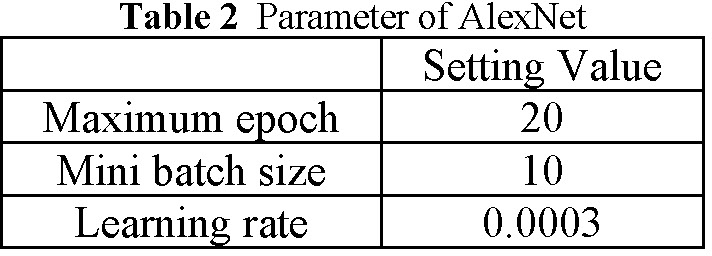
The training parameters are detailed in Table 2, and an example of the training results is illustrated in Fig. 1.
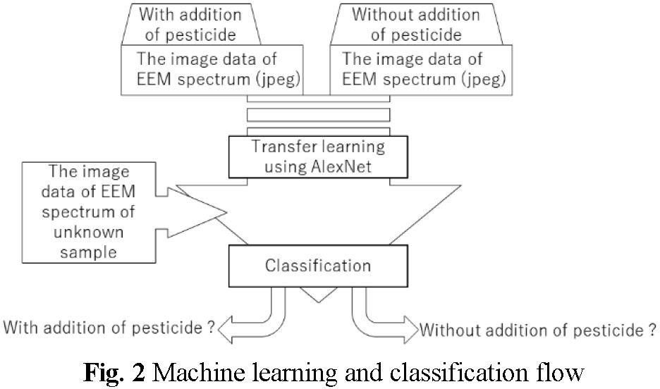
The training exercises were conducted by randomly selecting test data on five separate occasions. During each iteration, AI classified the test data as either “with addition pesticide” or “without addition pesticide”, utilizing 30 image datasets for both the “with addition pesticide” and “without addition pesticide” categories as verification data. Subsequently, metrics such as accuracy and the rate of correct answers for each assessment were meticulously recorded. Fig. 2 illustrates the process flow of machine learning and classification.

(7) Gradient-weighted class activation mapping 23) identification of critical areas for identification on EEM spectral images
In the context of employing machine learning for the classification of EEM, the critical areas and points that facilitate clarification need to be discerned and ascertained. Fig. 3 provides a visual elucidation for each prediction. This is achieved by generating a heat map through gradient-weighted class activation mapping (Grad-CAM). The heat map visually represents the segments of the input image that exert the most significant influence on the prediction, thereby offering a clearer understanding of the decision-making process of the algorithm.

(1) EEM spectrum of samples
All EEM spectra without the addition of pesticide, encompassing 28 samples, exhibited fluorescence peaks within the ranges of Ex 200-350 nm and Em 270-450 nm. Notably, the contours of these EEM maps predominantly assumed circular or oval shapes. When classified according to weather conditions, a distinct pattern emerged. For the samples collected on days characterized by fine weather, both on the day of sampling and the preceding day (5 samples), the EEM contour maps exhibited circular shapes with fluorescence peaks spanning the Em 270-420 nm region. Conversely, in instances where the weather on both the sampling day and the previous day was rainy (4 samples), the EEM contour maps were predominantly oval in shape, with fluorescence peaks extending over the Em 270-460 nm region. This observation suggests that under rainy conditions, the fluorescence peaks, as depicted by the EEM contour maps, tend to appear at longer wavelengths compared to those recorded on fine weather days. Fig. 4 exemplifies the EEM spectra for each weather condition.

(2) Changing of EEM spectrum by addition pesticide to river water samples
In this study, the highest concentration of pesticide added was 36 ng per 50 mL of sample, resulting in a cumulative amount of 1008 ng for the 28 species tested, corresponding to a concentration of 0.72 µg/L for each pesticide. Importantly, these concentrations, post-addition, were lower than the target thresholds specified for each pesticide in the Japanese Water Quality Standards. Fig. 5 presents the EEM spectrum of samples with and without the addition of pesticides as an illustrative example. In the EEM spectrum of samples to which pesticides were added, a noticeable trend was observed where the oval peak, particularly in the Ex range of 270-400 nm, expanded laterally. This expansion suggested a shift towards shorter wavelengths, though the change was not prominently visible. Similarly, when comparing samples with varying amounts of pesticides, no discernible changes that could be visually confirmed were evident.

(3) Classification by machine learning; the difference of EEM spectrum with/without addition pesticide
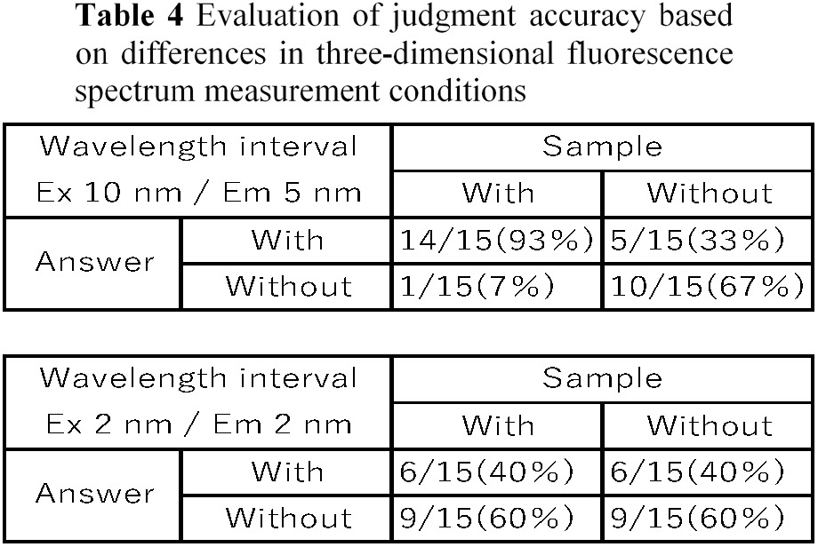
Table 3 presents the results of five verifications conducted using three sets of EEM image data, both with and without the addition of pesticides, as verification data. A total of 30 evaluations were conducted with a measurement wavelength interval of Ex 10 nm / Em 5 nm. Of these, the instances where the presence or absence of pesticide was accurately identified were 24 out of 30 (correct answer rate of 80%), and the accuracy ranged from 0.4848 to 0.7576. Conversely, when the measurement wavelength interval was reduced to Ex 2 nm / Em 2 nm, allowing for more precise EEM image data, the correct identification rate declined to 15 out of 30 times (50%), with accuracy ranging from 0.2727 to 0.5758. Table 4 details the evaluation of judgment accuracy for each sample. With the measurement wavelength interval extended to Ex 10 nm / Em 5 nm, the sensitivity, or the percentage of samples with pesticide addition correctly identified as “with” was 93%. The specificity, or the percentage of samples without pesticide addition correctly identified as “without,” was 67%. The positive predictive value (assuming a condition of 50% spiked sample) stood at 73%, while the negative predictive value reached 90.9%. Despite instances where samples with pesticides were misidentified as without, the results indicate that when the objective is detection, judgments can be made with a relatively high degree of accuracy. However, when the measurement wavelength interval was narrowed and data from more precise spectral measurements were used, both sensitivity and specificity dropped to 40% and 60%, respectively, and both the positive and negative predictive values stood at 50%. This highlights a significant reduction in judgment accuracy despite an increase in the volume of information.

(4) Grad-CAM
Grad-CAM was utilized to discern the regions of the EEM spectrum crucial for the image classification process in machine learning. The grad-CAM results are depicted as a heat map, where the red color signifies the primary areas of identification, and the blue color indicates regions of lesser significance. As illustrated in Fig. 6, two distinct types of heat maps were observed: (a) where the primary red area is concentrated in the center, and (b) where the primary red area is dispersed and not focused on a single point. In instances corresponding to Fig. 6(a), a propensity for correct answers was noted when the red areas were centrally clustered. Conversely, Fig. 6(b) demonstrates that a likelihood of incorrect answers arose when the main red area was not concentrated in a single point.

In this study, we measured the EEM spectrum of river water samples with low-concentration additions of a mix of 28 pesticide standards, as well as samples without any pesticide addition. These spectra served as training data for machine learning classification using AlexNet, aimed at distinguishing between samples with and without pesticides addition.
The maximum addition amount of each pesticide was 0.72 µg/L, with the 28 pesticides selected from those listed in the Water Quality Management Target Setting Items of the Tap Water Quality Standards -Individual Standards for Pesticides. The concentration of the spiked pesticides was considerably low, ranging from 1/10 to 1/1,000 of the standard values, except for Carbofuran (CAS No. 1563-66-2) and Fipronil (CAS No. 120068-37-3), which have the lowest standard values of 0.3 µg/L and 0.5 µg/L, respectively.
EEM spectrum image identification by the AI-machine learning environmental-spectrAI method demonstrated high sensitivity in screening for low concentration pesticide contamination in river water. This EEM method, akin to non-target analysis, offers advantages over other such methods, notably its cost-effectiveness and simplicity, requiring less expensive equipment and fewer pre-treatment steps. By integrating EEM and environmental-spectrAI methods, they can be utilized in river water monitoring, especially for precision measurements during disorder alerts.
The study employed two types of EEM images from river water samples: those spiked with a mix of 28 pesticide standards and those without pesticide addition, serving as training and test data. Additional considerations need the recovery rate of each pesticide, their fluorescence properties, and detection through environmental-spectrAI. This method shows promise in screening not only for pesticides but also for various chemical substances contaminating the environment, contingent on the preparation of training data.
Otani et al. 24) report on environmental sample analysis using AI based on numerical EEM data, highlighting the simplification and accuracy improvement possible through using EEM spectrum image data, including information on areas lacking fluorescence in the spectrum image for discrimination.
The study also explored measurements under two conditions: Ex 10 nm/Em 5 nm and Ex 2 nm/Em 2 nm wavelength intervals. While the Ex 10 nm / Em 5 nm interval yielded 1800 data points, the Ex 2 nm / Em 2 nm interval produced 22,500 points. Despite the significantly larger data set with the Ex 2 nm/Em 2 nm interval, accuracy in classification notably decreased. This outcome may be attributable to image data processing challenges.
The original spectral image data, with dimensions of 476 × 335 pixels, were compressed to 227 × 227 pixels for compatibility with AlexNet. This compression may have induced blurriness in the spectra, as observed in Fig. 7. The narrower contour line spacing at Ex 2 nm/Em 2 nm potentially led to AI misinterpretation, treating lines as filled-in images, which could account for the reduced accuracy when employing Ex 2 nm / Em 2 nm spectral images as training data.

In the process of classifying samples with and without pesticide addition using the environmental-spectrAI method, it has been determined that merely increasing the detail in the EEM spectrum measurement does not necessarily enhance the accuracy of image classification by AI. This observation, specifically within the context of the current AI system employing AlexNet, suggests that a measurement wavelength interval of Ex 10 nm / Em 5 nm might be optimal for the range tested in this study. Interestingly, similar experiments utilizing Inception-v3, capable of handling larger input data sizes than AlexNet, did not yield a significant improvement in accuracy. Instead, they resulted in a substantial increase in learning time (data not shown). This finding highlights that enhancing AI judgment accuracy requires improvements in both image resolution and AI analysis, rather than simply increasing EEM analysis precision and data volume. Therefore, establishing the optimal measurement accuracy is crucial.
In the AI analysis of the EEM spectrum images, incorrect answers were noted for samples with both the presence and absence of pesticides collected on a specific date (June 7th). This could be attributed to the types and quantities (background) of chemical substances, such as pesticides, present in the river water samples. As a result, concurrently measuring the background using LCMS and creating training data that considers these factors may lead to more accurate AI judgments.
Moreover, grad-CAM analysis revealed that the regions influencing the AI’s determinations in the EEM spectrum were those where the emission wavelength (Em, horizontal axis) was longer than the excitation wavelength (Ex, vertical axis), typically where fluorescence peaks were observed. This suggests that the AI’s discrimination of the EEM spectrum in this study relied on the fluorescence emitted by substances in the sample. Thus, the study’s objective of discriminating chemical substances in water was achieved with a high degree of reliability.
In validating the application of AI image classification to EEM spectrum image data, collecting a broader range of training data and establishing conditions applicable to various water qualities and sample types, such as river water, is crucial. Particularly, to minimize the background influence of environmental samples, enhancing the training data and setting precise conditions are crucial. This necessity becomes apparent when comparing results with those of Wu et al. 25), who achieved high accuracy in detecting food product falsifications, such as in sesame oil, where component similarities and minimal background variation exist. However, reports using environmental samples with significant background variations are scarce, and these variations may contribute to lower accuracy rates compared with the findings of Wu et al. 25). Employing a more recent network than AlexNet could improve discrimination accuracy of EEM spectral images. Conversely, AlexNet might still be compatible with current analyses of EEM spectral images, necessitating comparative verifications with other newer networks or higher-resolution images. Additionally, employing techniques such as Grad-CAM could help establish these conditions, evaluate the applicability of newer networks, identify cases where important identification regions do not overlap with spectral regions, and assess water quality under conditions conducive to validating identification regions.
In this study, the utilization of AI in conjunction with EEM spectrum image data of river water samples, both with and without added pesticides, enabled the determination of pesticide presence. This approach yielded high-accuracy judgments from a screening perspective. Should the accuracy of this method be further enhanced, it holds promise as a primary screening tool for analyzing river water samples. This potential highlights the method’s significance in environmental monitoring and the assessment of water quality.