Abstract
Cracks in civil engineering infrastructures, such as bridges, tunnels, and retaining walls, are common visual indicators of structural weakening. Damage to these structures can directly or indirectly impact human lives and property. In Japan, many of these infrastructures are ageing, making their maintenance a top priority to ensure safety. Traditional crack inspection methods for concrete structures often involve visual inspection using crack scales or gauges. However, this approach is time-consuming, labour-intensive, costly, and subject to the inspector’s judgement. In recent years, research has focused on leveraging Digital Image Processing techniques to address these challenges. This research aims to automate crack width monitoring by using YOLOv5 (You Only Look Once version 5) and the OpenCV library. Reflective targets are placed on either side of a crack to serve as a reference scale. The eight circles on the targets are automatically detected and measurement of the distance between the pair can be determined. The method was tested over a two-year period on a retaining wall in Tamano, Okayama, Japan, to demonstrate its applicability and feasibility. The results show that the model detects target circles with an accuracy of 95.9% and measures the crack movement. This method, compared to the manual approach currently used by the authors, significantly reduces crack width monitoring time, allowing for more frequent inspections and enhancing overall safety.
1. INTRODUCTION
Many civil engineering structures are essential to our economy and daily life, and their safety must be ensured. When a structure is built, it is inevitable that it will deteriorate over time. However, it is the responsibility of infrastructure managers to maintain these structures, preserving them and ensuring their continued safety. In recent years, the interdisciplinary field of Structural Health Monitoring (SHM) has emerged to address the challenges posed by ageing infrastructure worldwide1). SHM involves detecting damage in infrastructures across aerospace, civil, and mechanical engineering2, 3), as well as continuously monitoring their condition4).
Cracks in structures, while often a sign of deterioration, can provide valuable insights into the condition of the material. While some minor cracks, such as those caused by thermal expansion, are not dangerous5, 6), cracks remain one of the most common indicators of damage when assessing concrete structures. The pattern, orientation, type, number and width of cracks can reveal important information about the internal stresses and forces affecting the structure as well as its durability7, 8, 9). This crack data can then be used by decision-makers to guide maintenance efforts, adjust load capacities, or implement other necessary changes to ensure the structure’s safety. Therefore, it is important to detect cracks within a reasonable time and monitor them frequently2).
To track the development of cracks, visual inspection is often the first step carried out by experienced personnel. According to the Bridge Inspectors Reference Manual10), all visible cracks in concrete structures must be recorded, noting their location, type, width, and length. This initial analysis helps determine whether a more detailed investigation is needed. For measuring crack width, a crack gauge (a type of ruler with a range from 0.03mm to 2.20mm) is placed on the crack to measure its width, while the shape is outlined with chalk. Inspectors also create manual sketches of the cracks.
While this traditional visual inspection method has been the go-to approach for years, it is time-consuming, costly, and difficult to replicate11). Moreover, performing visual inspections requires access to the structure, which can disrupt service operations. To minimise disruptions, inspections are often carried out at night, but this comes with limited time frames and increased risks for inspectors12). Adding to the challenge, Japan is experiencing a decline in its construction workforce due to an ageing population and low birth rates. Furthermore, because inspections are done manually, they are subject to individual judgement and errors caused by human fatigue1). These challenges have made regular monitoring more difficult.
In response to these limitations, the use of Digital Image Processing (DIP) techniques has gained momentum since the 2000s, fuelled by advances in computers, cameras, smartphones, and more recently, Unmanned Aerial Vehicles (UAVs). This approach uses images and computer algorithms to analyse crack details in infrastructure. With a growing number of publications on crack detection, classification, and width measurement13, 14), it is evident that a new, more effective method for crack inspection is not only sought after but has already proven to be a promising alternative.
Although cameras have provided an easy way to acquire images for crack inspections, and earlier challenges such as storage capacity15, 16) have been addressed, new challenges have emerged. Analysing these images manually remains arduous and time consuming. To overcome this, Convolutional Neural Networks (CNNs) have gained traction in automating the process. CNNs, a type of deep learning algorithm designed for image classification and object recognition, have been employed by several researchers to detect cracks17, 18), classify them5) and measure their width19). Given their robust performance and high accuracy, CNNs are a suitable solution for crack inspection.
One popular CNN architecture for real-time object detection is You Only Look Once (YOLO)20). As a one-stage detector, YOLO makes predictions in a single pass through the network, bypassing the Region Proposal Network (RPN) stage. It is especially known for its speed, ease of use and high accuracy.
For example, Shao et al.21) utilised YOLOv3 to detect the cracks in road pavement. After comparing key metrics, precision, recall, and average Intersection over Union (IOU), among YOLOv3, SDDNet, YOLOv4 and YOLOv5, they found YOLOv3 (75.29%) outperformed the SDDNet model, but lagged behind YOLOv4 (85.48%), and YOLOv5 (83.18%) in terms of precision.
Yu et al.22) combined YOLOv5 with image processing techniques for crack detection and quantification. YOLOv5 was used for the crack classification and location, while an image processing method based on a region-connected component search algorithm was applied for crack quantification. By augmenting their dataset to increase the training data, their method achieved high accuracy, with detection precision of 92.0%, recall of 97.5%, and a mean average precision (mAP) of 98.7%. The authors were also able to detect and quantify cracks as small as 0.15mm.
Similarly, Inam et al.23) used YOLOv5 to detect cracks in bridges using a combined dataset of images from Pakistan and the public SDNET2018 dataset. YOLOv5 has four different model variants, each with varying sizes: small (s), medium (m), large (l) and extra-large (x). The authors evaluated the performance of the YOLOv5s, YOLOv5m, YOLOv5l models using key metrics, precision, recall, and Mean Average Precision (mAP). The results showed that the YOLOv5m model achieved the highest performance (99.3%), followed closely by YOLOv5l (99.1%) and YOLOv5s (97.8%).
The results of these studies have demonstrated the effectiveness of the YOLO family of models for crack detection. These studies focused on detecting and quantifying the cracks. In various countries, different standards are set for the maximum allowable crack width. For example, the standard crack width limit is less than 0.5 mm in some countries24), while in Chile, a crack is defined as larger than 5mm (cracks less than 5mm are defined as fissures)25). According to the European Organisation for Technical Approvals (EOTA)26), the maximum allowable crack width for post-tensioned structures is 0.25mm. In contrast, Japan does not define specific numerical criteria for crack width or length. Instead, maintenance urgency ratings are used24). Given that cracks may expand very slowly over time, continuously monitoring their behaviour is essential 27,12).
Building on previous work, this study enhances the crack width monitoring system developed by Nishiyama et al.28), which utilised perspective transformation for crack displacement measurement. Their approach involved placing a pair of reflective targets (with four circular glass beads) on either side of a crack to measure the displacement. By calculating the centroid from a binarised image of the target circles’ centre, the distance between the two points can be measured over time, capturing the displacement of the crack width. However, this method relied on a computer programme, Image Measure(c), that required human intervention to determine the optimal threshold value. This process is time-consuming and tedious.
With the rapid advancements in deep learning techniques, this study aims to integrate YOLOv5 with image processing methods, eliminating the need for human calculations. As far as the authors are aware, there are no existing literature with this technique, marking the originality and innovation of this research. By automating the process, this research has the potential to not only reduce the time required for inspections but also improve the objectivity of the results. Using targets that are affixed to the monitoring surface enabled the measurement of the same cracks at the same location over a two year period. The method is both low-maintenance, fast and cost-effective. First, the targets are detected by the YOLOv5 model. Then using the OpenCV library, perspective transformation is performed based on the centre coordinates.
Following this, binarisation is applied to find the exact centre of gravity. Finally, the distance between the targets is calculated. This proposed method was validated using images taken of a retaining wall in Okayama, Japan.
The remainder of this article is organised as follows: Section 2 describes the equipment used for image acquisition and the methodology used including a brief explanation of YOLO. It also includes the results obtained from the YOLOv5 model. Section 3 demonstrates the application of the developed method to measure crack displacement over a two-year period in Okayama, Japan. Section 4 discusses the findings and Section 5 concludes the paper and suggests improvements for future research.
2. MATERIALS AND METHODS
(1) Principle of measurement system
The principle of this measurement system is explained in detail in Nishiyama et al.28), but a brief overview is provided in this section.
The reflective targets used in this research have four glass beads precisely positioned, ensuring light reflects the beads when the image is taken. The two- dimensional coordinates of the centre of each circle are determined by calculating the centre of gravity of the white areas in the target.
Using perspective projection, based on the collinearity condition, an image can be taken from any angle, allowing for the front facing view to be obtained, which is one of the merits of this developed measurement system. For more details on the system, refer to the paper by Nishiyama et al.28).
(2) Workflow
The method developed in this research aims to measure the distance between two reflective targets using a deep learning algorithm. Fig.1 illustrates the schematic workflow of the process resulting in the calculated measurement. This study is divided into 4 main tasks: 1) Image Acquisition 2) Data pre- processing 3) Model Training and Testing and 4) Distance calculation. Each step is explained in detail below.
(3) Image Acquisition
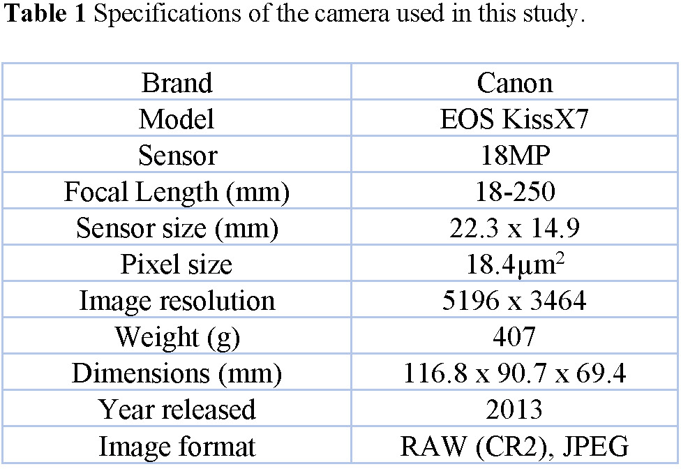
The accuracy and quality of the output image are directly influenced by the type of camera used29,30). The type of camera chosen depends largely on the specific objectives of the study. For crack detection, cameras with high resolutions are typically preferred 1,17,31). Digital Single Lens Reflex (DSLR) cameras are commonly used in digital photogrammetry applications32). DSLRs are very versatile offering the advantage of interchangeable lenses33). Furthermore, the large image sensor size of DSLRs allow for better light capture, resulting in higher image quality. In this study, the DSLR Canon EOS Kiss X7 (also known as the EOS Rebel SL1 or EOS 100D; hereafter referred to as Canon Kiss X7) was used (Fig.2). The choice of this camera was based primarily on its availability, rather than technicality. Table 1 presents the camera’s specifications.
a) Dataset
Images of the target pairs (both 55 x 55 mm and 110 x 110m size targets) were captured at various locations, including on a bridge pier, affixed to a micrometre, and outdoors surrounding actual cracks, at distances up to 15m. This variety of settings allowed for the capture of images under different conditions such as varied lighting and background objects like trees and cars. A total of 316 images were collected, which were then split into training (66%), validation (18%) and testing (16%) datasets.
For the testing dataset, the images were captured from an experiment conducted outside the laboratory. Using a measuring tape and a professional laser measure (GLM 50-27 CG), images were taken at distances of 1, 3, 5, 7, 10 and 15 metres, at angles of 0°, 22° and 45°, free hand. All images were taken with a focal length of 250mm. The micrometre was moved in increments of 0.2mm to assess the accuracy of the displacement measurements. Fig.3 shows the shooting positions. The experiment was conducted between 8 am and 12 noon, under sunny conditions. Table 2 shows the pixel density of the target circles at varying distances.
(4) Data pre-processing
For object detection machine learning models, the training and validation datasets require precise annotation and labelling. Using the labelImg tool (https://github.com/HumanSignal/labelImg), each reflective white circle on the targets was manually annotated with the YOLO bounding box method and labelled with the class “target” (Fig.4). This process resulted in a total of 1659 annotated circles for training, 448 for validation and 416 for testing. Additionally, 55 images (440 annotated circles) collected during the site visits were used for testing purposes.
5) Model Training and Testing
a) YOLO
Input images for deep learning models must be of a consistent size to ensure effective training. YOLOv5 automatically resizes images to the default resolution of 640 × 640 pixels during pre-processing. In this research, the dataset was not augmented, as the targets are specific objects that could be easily distorted through operations such as cropping and scaling. Fig.5 shows examples of images from each dataset. YOLO is a real-time object detection system capable of both localising and classifying objects in images or videos.
It was introduced by Redmon20) to solve the previous work that repurposed image classifiers (such as Region-based Convolutional Neural Network (R-CNN)) to perform the detection. Instead of using multiple steps, YOLO predicts both bounding boxes and class probabilities directly from the input image in a single pass. This design made YOLO faster than its predecessor, R-CNN.
Since its introduction, it has evolved significantly, with continuous improvements in model architecture, training strategies, and performance. It has become more accurate, efficient and user-friendly. The latest version, YOLOv11, was released in September 2024, and continues the family model’s focus on improving both accuracy and speed.
For the purposes of this research, YOLOv5 (2020), developed by Ultralytics, was used. There is no paper is available for this version of the network. YOLOv5 offers four variants: small (s), medium (m), large (l) and extra-large (x). The YOLOv5s variant was automatically selected when the model was executed, based on the dataset size. This s variant is the lightest and fastest in the YOLOv5 family, allowing for faster processing times though it may sacrifice on performance when compared to the larger models23). This paper will not delve into the full details of the YOLOv5 architecture, as comprehensive explanations are available in existing literature22, 23). In brief, YOLOv5 features a backbone network for feature extraction, a neck network for feature aggregation, and a head network for making the final predictions. For further details, readers are referred to the aforementioned sources.
b) Hardware and software configurations
The experiment was implemented using Python programming language (version 3.12.7) with the PyTorch deep learning framework34). The computer system utilised an AMD Ryzen 9 9950X processor with 16 cores and a base clock speed of 4.30GHz. It was equipped with 64 GB of RAM which was sufficient memory for processing the dataset used in this research. The operating system was Windows 11 Pro (64-bit). For faster processing and reduced training times, the use of a GPU is often recommended13, 35). In this study, the NVIDIA GeForce RTX 4090 24GB-GDDR6X GPU was used, enhancing processing efficiency and optimising training performance, reducing the training time to approximately 4 hours.
c) Training
The labelled data was input into the YOLOv5 model for training. The batch size was set to 32, and the model was trained for 230 epochs. YOLOv5 uses Stochastic Gradient Descent (SGD) as the default optimiser. The learning rate was adjusted dynamically throughout the training process using a scheduler, either cosine or linear, depending on the configuration. Fig.6 shows examples of detected and misdectected circles. Fig.7 illustrates the model’s performance during both training and validation phases. Fig.8 shows the performance during testing.
d) Performance Evaluation
The performance of the model was evaluated using standard metrics: accuracy (1a), precision (1b), recall (1c) and F1 score (1d).
TP = True Positives; TN = True Negatives; FP = False Positives; FN = False Negatives.
Accuracy is defined as the ratio of true predictions to the total number of predictions made.
Precision is the correct predictions.
Recall measures the proportion of actual positives that are correctly identified by the model.
F1 score is the mean of precision and recall. A high
F1 score indicates both high precision and high recall.
Mean Average Precision (mAP) takes into account both the precision and recall. mAP_0.5 is the IoU threshold of 0.5.
e) Relationship between RMSE, Standard Deviation and the shooting distance
Two accuracies were used to evaluate the system: Root Mean Squared Error (RMSE) and Standard Deviation.
Where n represents the number of measurements. A smaller standard deviation indicates greater stability in the observation results under the same conditions.
(6) Distance Calculation
To calculate the distance between the targets, OpenCV’s Library was utilised. OpenCV is an open- source computer vision library developed by Gary Bradski in 199936). It is widely known for its ease of use but applicable to complex scenarios.
For this research, the primary functions used included threshold operations (e.g. cv2.threshold), drawing functions (e.g. cv2.circle, cv2.line), image transformations (cv2.getPerspectiveTransform) and various other utilities for reading and writing images.
a) Binarisation
After the model successfully detects the circles, the centre coordinates of each detected circle (Centrex and Centrey) are calculated by averaging the maximum and minimum x and y coordinates of the bounding box (Fig.9A), as follows:
Where x1 and y1 represent the maximum x and y coordinates of the bounding box respectively, and x2 and y2 represent the minimum x and y coordinates, respectively. It is important to note that if the bounding box is displaced relative to the circle, the calculated coordinates will also be shifted from the true centre and would require correction.
The target image is binarised by applying a threshold intensity value (Fig.9B), which separates the image into white and black areas, using OpenCV’s cv2.threshold () function. In this process, pixels with an intensity greater than or equal to the threshold are set to 255 (white), while pixels with an intensity below the threshold are set to 0 (black). After binarisation, the white regions (255) are considered as the object of interest. The average coordinates of the white pixels are then calculated to determine the centre of gravity (also referred to as the centroid) of the white region. The centre of gravity is the point that represents the average position of all the white pixels, or the point of concentrated weight.
b) Perspective Transformation (Homography)
Perspective transformation, also known as homography, is a type of projective transformation that is used to map the coordinates of points from one plane to another. This is a type of linear transformation that maps points into points, line into line and planes into planes, making it ideal for transforming images. Specifically, it maps points in the camera coordinate system to the object space coordinate system.
In this research, the coordinates of four reference points (i.e. the centres of four circles on a target) are used to perform the perspective transformation.
To determine the correct order of the circles for the perspective transformation, first, the longest edge among the eight centre points is selected to serve as the x-axis of the object space (Fig.9C). This edge defines the primary axis along which the transformation will take place. Then the circles are labelled according to the following order (Fig.9D): Point No.1: The leftmost point of the longest edge (i.e., the point with the smallest x-coordinate). Point No.2 and No.3 are compared and the larger of the two y coordinates is Point No.2, the next is No.3. Point No.4 is the next largest x-coordinate along the line. These four points are the source coordinates (src) for the perspective transformation. These points represent the location of the target on the original image before transformation. The destination coordinates (dst) correspond to the positions of the same points in the transformed image, which give the view of the target from the front.
Using cv2.getPerspectiveTransform() function in OpenCV, the perspective transformation matrix is computed (Fig.9E). This function takes the source coordinates (before transformation) and the destination coordinates (after transformation) and calculates the homography matrix that will map the original coordinates to the transformed ones.
After obtaining the perspective transformation matrix, transformation is done to the entire image using the cv2.warpPerspective() function, which warps the original image based on the calculated transformation matrix (Fig.9F).
However, since only four of the eight coordinates are transformed during the process described above, the remaining coordinates are transformed using a projective transformation matrix and transferred onto the image. These coordinates are hereafter referred to as the transformed coordinates.
c) Binarisation2
As the transformed coordinates may not accurately capture the centre of gravity of the circle, the final distance calculation accuracy is ensured by recalculating the precise centre of gravity.
After the projective transformation, the image is binarised using the cv2.threshold() function, with an appropriate threshold value set based on the image. A circular mask is created around the centre of the transformed coordinates, and this mask is expanded. This is the same process as the aforementioned binarisation process (Fig.9B, inset). The process terminates when all pixels within the circle mask are black, effectively identifying the radius of the circle (Fig.9G).
The centre of gravity is then determined by calculating the average coordinates of all white pixels within the circle mask. These coordinates are used as the final centre of gravity for the circle.
d) Calculate the distance
Using the same labelling system as before, the circles are relabelled as Point No.1, No.2, No.3 and No.4. Point No. 5 will be the point directly opposite Point No.4 (Fig.9H). The distance between Points No.4 and No.5 is then calculated (Fig.9I), with the understanding that the true distances between Points No.1 and No.2 as well as between Points No. 1 and 3 are 35mm.
(7) Otsu Method
There have been many studies that have utilised the Otsu Method to detect and measure cracks22,37,38). The Otsu algorithm, first proposed by Nobuyuki Otsu in 1979, is commonly applied in OpenCV using the cv2.threshold() function for thresholding. Typically, thresholding is done by manually setting the threshold. However, to automate this process, the Otsu method can be applied by passing the cv2.THRESHOTSU as the value of the thresholding flag in the function. This allows the method to automatically determine the optimal threshold value for binarisation. The effectiveness and automation of this method are dependent on how well the optimal threshold value is determined37). For this reason, the authors aimed to compare the results of using the Otsu Method with those obtained by standard thresholding. In standard thresholding, the threshold value is selected by trial and error, testing values between 0 and 255 and adjusting the threshold based on how well the circles’ edges are detected. This process continues until the results are optimal.
3. APPLICATION
a) Location and Geology
Tamano City, located to the southernmost tip of Okayama Prefecture, Japan, is a small, coastal town (Fig.10). Established in 1940, the city is characterised by its rugged, steep terrain with approximately 60% being classified as mountainous and primarily composed of granite39,40). Originally, an agricultural-based city, Tamano transitioned to industrial manufacturing in the early 1900s, becoming known for its shipbuilding industry and home to one of Japan’s largest shipyards.
Uno Port serves as a key maritime hub for the Seto Inland Sea and a major gateway to Okayama Prefecture. However, the city is prone to natural hazards, particularly sediment disasters and landslides, often triggered by heavy rainfall and typhoons. In response to this, the Tamano City Crisis Management Division issued a sediment disaster index map in July 2014. Due to its vulnerability to these natural hazards, Tamano City was selected as the focus of this research.
The retaining wall (Fig.11) under investigation is located near the end of the National Route 30, a major highway connecting Okayama to Takamatsu, Japan.
This highway is critical to the country’s transportation infrastructure. Any disruption to this route could have significant repercussions on both the economy and the daily lives of millions of people. Therefore, monitoring crack width in the retaining wall is essential to ensure the continued stability and safety of this national highway.
b) Climate characteristics
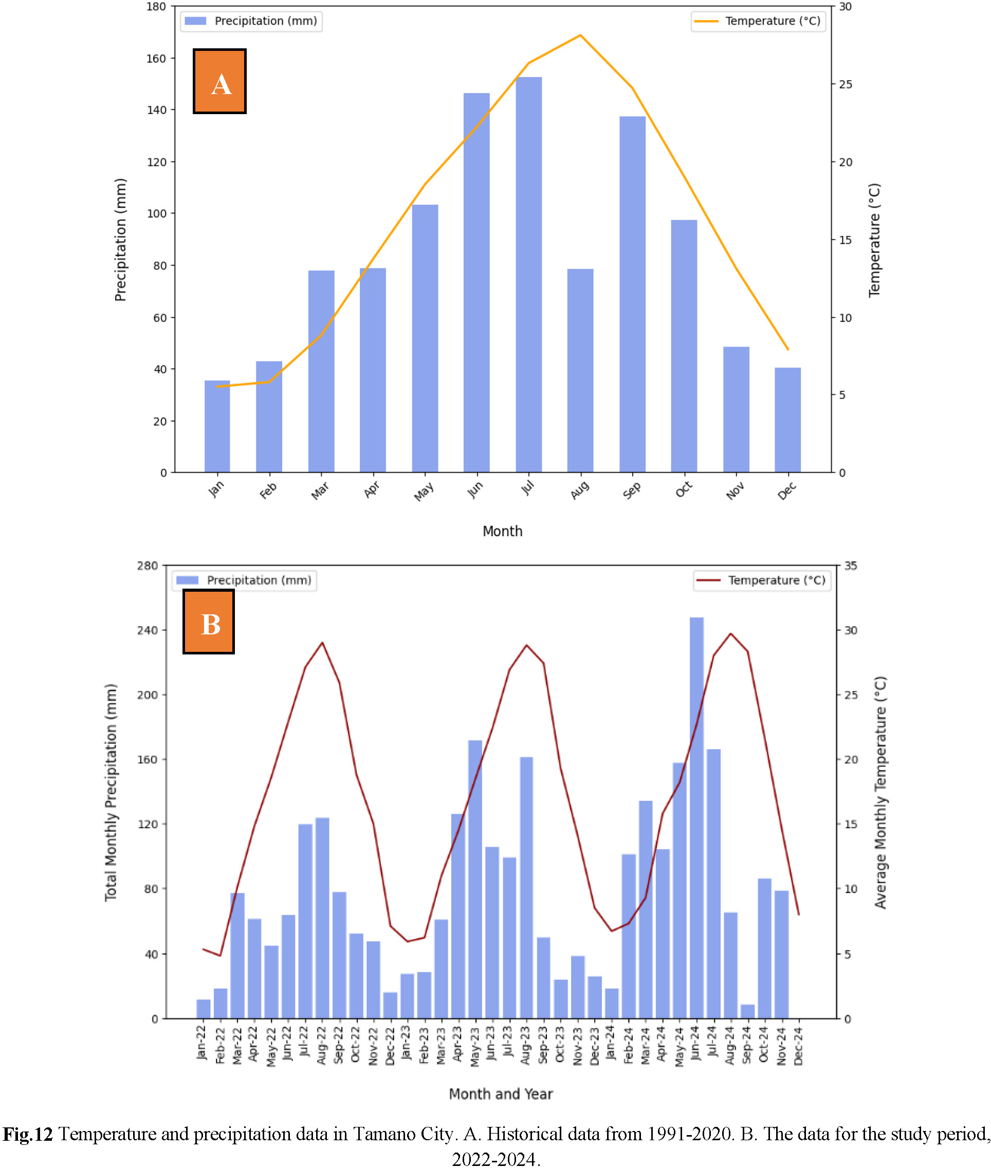
Tamano City has a humid subtropical climate. According to the Japan Meteorological Agency41) (JMA), the average precipitation and temperature from 1991 to 2020 (30 year period) were 1038.5mm and 16.1°C respectively. Fig.12A illustrates the average monthly precipitation and temperature data for the same period. The figure reveals that rainfall is concentrated from June to September, highlighting the region’s rainy season. In Japan, the typhoon season runs from May to September, with peak activity typically occurring in August and September. Fig.12B shows the total monthly rainfall data and the average monthly temperature data for the period of this research (2022-2024). In 2023, which is when the majority of the data were collected, the cumulative precipitation was 917.5mm.
c) Image acquisition
To investigate the soundness of the retaining wall, cracks were photographed from December 2022 to December 2024, covering multiple seasons, experiencing a range of temperatures and rainfall conditions. The data collection was mainly done in the morning hours (Table 4). According to the MLIT inspection report, the retaining wall is approximately 15m in height and is divided into three sections: the first level (where the targets were affixed, less than 5m in height), the second level (slope) and the third level (residential land). Reflective targets were placed at 3 positions, numbered 4, 2 and 5 (Fig.13) with cracks at points 2 and 5 extending to the top of the wall.
Images were captured free hand at varying angles and distances, using focal lengths of 18m and 51mm for a distance of 1m. The results presented in this paper are limited to these parameters.
4. RESULTS AND DISCUSSION
a) Performance of YOLOv5 Model
According to Fig.8 and Table 5, the YOLOv5 model demonstrated accurate circle detection at distances ranging from 1m to 7m. However, as the distance increased to 10m and 15m, the model’s accuracy decreased, with detection rates of 0.984 and 0.781, respectively. We noted false detections at distances of 1m and 5m. The model emphasised background features that were similar to the target. As can be seen from Table 2, at longer distances, the pixels of the circles become smaller, which increases the likelihood of misdetection (false negatives). From previous research28), it is known that as the distance and/or angle of photo acquisition increase, the accuracy and precision decreases. Similarly, when the distance and angle of image acquisition was increased, the model’s ability to detect the circles significantly decreased. From distances 1-10m, the YOLOv5 model was capable of detecting the circles at 45°, but at a distance of 15m, most circles at that angle could not be detected at all. Therefore, if the distance and/or angle is increased, the detection accuracy of the circles will decrease.

Several different attempts were conducted to evaluate the model’s performance on the dataset. First, the model was trained with a larger dataset. The training dataset contained 2,848 circles, with 560 used for validation and the same 416 circles for testing, over 200 epochs. The model took a longer time to train, and the accuracy decreased, likely due to overfitting caused by the excessive amount of data. Additionally, the default optimiser for YOLOv5 is SGD, which was used in the initial experiment. However, the Adam optimiser, known for its faster convergence and efficient performance42), was also tested. Adam helps adjust the network’s weights to minimise loss. In this study, though the number of epochs was reduced from 230 to 200, the use of Adam resulted in decreases in accuracy, precision, recall, and F1 score. However, further experimentation with optimisers should be explored by varying the hyperparameters.
b) Results of verification method
In the Fig.14, 15 and 16, the cumulative crack displacement measurement is plotted against temperature and time for crack 4, 2 and 5. According to Fujiu et al.43), if environmental conditions are not considered in maintenance plans, appropriate repairs may not be able to be set. As seen in Fig.14, the displacement is steady over the 2 year period, which is consistent with the visual inspection report by the MLIT, measured every 2 years since 1998.
The Otsu and manual methods show very similar trends, while the AI method (without Otsu) exhibits slight differences. For Fig.15 and Fig.16, the crack extends to the second level which could have an effect on the crack on the first level. The temperature has also been shown to influence crack behaviour40). The figures show that the crack opened in colder temperatures and closed in hotter temperatures. Okazaki et al.44) stated the effect of high rainfall on crack propagation.
Although Fig.15 and Fig.16 show fluctuations in the displacement during the two-year observation time, there was no significant progression of the crack width, and we consider these cracks (2 and 5) to be stable.
In Fig.14 and Fig.16, increased rainfall during the June-July period contributed to a slight rise in displacement measurements. Additionally, the soil load-bearing capacity of the retaining wall can also influence crack movement12), although this was not investigated in this research.
Fig.17 shows a scatter plot of cumulative AI and AI + Otsu against cumulative manual measurements. While Figs.14 ,15, and 16 suggest that the Otsu method is closer to the manual method than AI with standard thresholding, Fig.17 indicates that the standard thresholding method is, in fact, closer to the manual measurements. The slope of the standard thresholding method is nearer to 1, and its smaller intercept suggests a better alignment with the manual measurements. Although the difference between the two methods is minimal (5 × 10⁻⁴), the Otsu method is too inconsistent to be considered a reliable alternative at this point. For example, Fig.14 is missing data for Otsu method calculation for December 2024, and Fig.15 is missing data for February and June 2023 because the perspective transformation could not be performed, which will be explained in the next section.
c) Otsu Method
The Otsu method was compared with the standard threshold function, cv2.threshold() (Fig.18A), to enhance the automation of this research, thereby increasing the efficiency of deformation measurement. However, when the original image (Fig.18B) was binarised using the Otsu method (Fig.18C), followed by the perspective transformation, the image failed to successfully perform the transformation. This resulted in an inaccurate distance measurement of 87.07mm, compared to 44.17mm when the threshold was manually set at 200 using the cv2.threshold() function. The threshold calculated by the Otsu method was unable to properly separate the black and white regions of the target due to its consideration of the entire image, which included both the target and the concrete background. The Otsu method attempts to find a single threshold value to distinguish the foreground from the background. However, for Otsu to work effectively, the foreground and background, i.e., the black and white areas of the target, must be clearly separable. In this study, the brightness of the pixels outside the target interfered with the binarisation process (Fig. 18C).
Fig.19 shows a histogram of the brightness of all pixels in the image that could not be successfully binarised using the Otsu method and plots the threshold value obtained by the Otsu method and the threshold value that successfully binarised the image (hereinafter referred to as the true value). The figure shows that the threshold value calculated by the Otsu method is 65 smaller than the true value, which is due to the influence of the background (i.e. concrete) as mentioned earlier. However, having to choose a suitable threshold value is a shortcoming of this research method.
Given that these images have varying lighting complexities, with areas of underexposure or overexposure1), the Otsu method, may not be well-suited for them. Instead, methods like Niblack or Wolf3), both local adaptive thresholding methods, could be more effective for handling images with varying illumination.
Yu et al.22) stated that, in crack detection research, the use of Otsu and multiple filtering methods in image processing was performed on simple backgrounds, and therefore, these algorithms may fail in real-world applications. Similarly, in this research, the background was relatively simple, but in more complex scenarios, such as backgrounds with graffiti, paint, chalk, or obstacles, the binarisation process could fail.
5. CONCLUSION
In this research, reflective targets with scaled circles were used to perform perspective transformation and calculate the distance between the pair of targets using the YOLOv5 model and the OpenCV library. The detection model and distance measurement were validated with data collected between December 2022 and December 2024 in Tamano, Okayama, Japan.
The use of targets to measure crack displacement is advantageous as it allows for constant monitoring of the same crack over time. While deep learning methods can directly measure the crack width22), factors such as lighting, background noise and other environmental conditions can complicate accurate detection.
The YOLOv5 model was able to obtain a total accuracy of 95.9% for distances ranging from 1m to 15m. Additionally, when compared to manual measurement methods, the calculated distances were consistent for most months. The crack displacement is steady and the movement over the last two years has been less than 1mm. This model was trained, validated and tested on a private dataset created by the authors. However, as noted by Avendano et al.3), models trained on such specific datasets may achieve high accuracy but perform poorly on datasets with different characteristics. While the targets used in this research are unique to the study, incorporating additional features, such as varying shapes, could potentially improve detection and accuracy.
This research is limited to investigating only the crack width, although other factors such pattern, orientation, type, number, also provide important insights into the condition of the structure. Generally, crack width is considered the best indicator of deterioration18), 22). A widening crack allows moisture, salts and water to penetrate, which accelerates its growth. Hence, as mentioned earlier, some countries have an allowable limit for crack width.
Another limitation of this research is its reliance on a GPU, which can be costly. However, some researchers, including Inam et al.23) and Zoubir et al.45), have used Google Colab, which provides free access to GPUs and has been sufficient for their needs. Bach and Tung46) used Kaggle which was also adequate for their research.
For future improvements, automating the threshold determination process is crucial to eliminate manual intervention. Binarisation is a key part of the process for this developed method. Since the Otsu method was faster than the standard thresholding method, finding ways to enhance its performance in this research is essential. Drawing a bounding polygon around the target could help remove the background, potentially improving the Otsu method’s results. Additionally, the Niblack or Wolf methods should be explored to compare with the Otsu method. These methods, as well as, ensuring the centralisation of the circle is appropriate, is necessary for improving this study.
Images were captured during periodic visits to the structure, typically every couple of months. The image acquisition process was generally completed within 15 minutes. However, data analysis required additional time. To further reduce inspection and analysis time, the authors are working on developing an automated system for image acquisition and analysis using Pan- Tilt-Zoom cameras.
Acknowledgments
The authors would like to acknowledge the use of ChatGPT for assistance with code writing in the methodology section, which was reviewed by the supervisor, as well as a writing assistant in proofreading and grammar checking.
References
- 1) Świt, G., Krampikowska, A., & Tworzewski, P.: Non- destructive testing methods for in situ crack measurements and morphology analysis with a focus on a novel approach to the use of the acoustic emission method, In Materials., Vol. 16, Issue 23, 2023.
- 2) Farrar, C. R., & Worden, K.: An introduction to structural health monitoring, Philosophical Transactions of the Royal Society A: Mathematical, Physical and Engineering Sciences, Vol. 365, No.1851, pp. 303-315, 2007.
- 3) Avendaño, J. C., Leander, J., & Karoumi, R.: Image-based concrete crack detection method using the median absolute deviation, Sensors, Vol. 24, No.9, pp. 2736, 2024.
- 4) Qayyum, W., Ehtisham, R., Bahrami, A., Mir, J., Khan, Q. U. Z., Ahmad, A., & Özkılıç, Y. O.: Predicting characteristics of cracks in concrete structure using convolutional neural network and image processing, Frontiers in Materials, 10, 2023.
- 5) Bhowmick, S., Nagarajaiah, S., & Veeraraghavan, A.: Vision and deep learning-based algorithms to detect and quantify cracks on concrete surfaces from UAV videos, Sensors (Switzerland), Vol. 20, No.21, pp. 1-19, 2020.
- 6) Nyathi, M. A., Bai, J., & Wilson, I. D.: Concrete crack width measurement using a laser beam and image processing algorithm, Applied Sciences (Switzerland), Vol. 13, No.8, 2023.
- 7) Kim, H., Sim, S. H., & Cho, S.: Unmanned Aerial Vehicle (UAV)-powered concrete crack detection based on digital image processing, 6th International Conference on Advances in Experimental Structural Engineering, 2015.
- 8) Valença, J., & Júlio, E. S.: Assessment of cracks on concrete dams by image processing. The case-study of Itaipu dam, at the Brazil-Paraguay border, INGEO 2017- 7th International Conference on Engineering Surveying, 2017.
- 9) Li, S., & Zhao, X.: Automatic crack detection and measurement of concrete structure using convolutional encoder-decoder network, IEEE Access, Vol.8, pp. 134602- 134618, 2020.
- 10) Bridge Inspectors Reference Manual, [National Highway Institute], 2022.
- 11) Parente, L., Falvo, E., Castagnetti, C., Grassi, F., Mancini, F., Rossi, P., & Capra, A.: Image-based monitoring of cracks: effectiveness analysis of an open-source machine learning-assisted procedure, Journal of Imaging, Vol. 8, No.2, 2022.
- 12) Belloni, V., Sjölander, A., Ravanelli, R., Crespi, M., & Nascetti, A.: Crack Monitoring from Motion (CMfM): Crack detection and measurement using cameras with non- fixed positions, Automation in Construction, Vol. 156, 2023.
- 13) Munawar, H.S., Hammad, A.W.A., Haddad, A., Soares, C.A.P., Waller, S.T.: Image-based crack detection methods: a review, Infrastructures, Vol.6, No.8, p.115, 2021.
- 14) Hamishebahar, Y., Guan, H., So, S., & Jo, J.: A comprehensive review of deep learning-based crack detection approaches, In Applied Sciences (Switzerland), Vol. 12, Issue 3, MDPI, 2022.
- 15) Ju Lee, B., Hoon Shin, D., Won Seo, J., Deuk Jung, J., & Yeong Lee, J.: Intelligent bridge inspection using remote controlled robot and image processing technique, 2011 Proceedings of the 28th ISARC, pp. 1426-1431, 2011.
- 16) Sharma, A., and Mehta, N.: Structural Health Monitoring using image processing techniques-a review, International Journal of Modern Computer Science, Vol. 4, No. 4, 2016.
- 17) Minami, T., Urata, W., Fujiu, M., Fukuoka, T., Sagae, M., Suda, S., & Takayama, J.: Development of automatic concrete cracks detection system using average shifted mesh, In Journal of the Eastern Asia Society for Transportation Studies, Vol. 13, 2019.
- 18) Nyathi, M. A., Bai, J., & Wilson, I. D.: Deep Learning for concrete crack detection and measurement, Metrology, Vol.4, No.1, pp. 66-81, 2024.
- 19) Guo, Y., Wang, Z., Shen, X., Barati, K., & Linke, J.: Automatic detection and dimensional measurement of minor concrete cracks with convolutional neural network, ISPRS Ann. Photogramm. Remote Sens. Spatial Inf. Sci., X- 4/W3-2022, pp. 57-64, 2022.
- 20) Redmon, J., Divvala, S., Girshick, R. and Farhadi, A.: You Only Look Once: unified, real-time object detection, arXiv:1506.02640, 2016.
- 21) Shao, C., Zhang, L., and Pan, W.: PTZ camera-based image processing for automatic crack size measurement in expressways, IEEE Sensors Journal, Vol. 21, No.20, pp. 23352-23361, 2021.
- 22) Yu, L., He, S., Liu, X., Jiang, S., and Xiang, S.: Intelligent crack detection and quantification in the concrete bridge: a deep learning-assisted image processing approach, Advances in Civil Engineering, Vol.2022, No. 1, 2022.
- 23) Inam, H., Islam, N. U., Akram, M. U., & Ullah, F.: Smart and automated infrastructure management: a deep learning approach for crack detection in bridge images, Sustainability (Switzerland), 15(3), 2023.
- 24) Jeong, Y., Kim, W. S., Lee, I., & Lee, J.: Bridge inspection practices and bridge management programs in China, Japan, Korea, and U.S., Journal of Structural Integrity and Maintenance, Vol.3, No.2, pp. 126-135, 2018.
- 25) Forcael, E., Román, O., Stuardo, H., Herrera, R.F., Soto- Muñoz, J.: Evaluation of fissures and cracks in bridges by applying digital image capture techniques using an Unmanned Aerial Vehicle, Drones, Vol. 8, No. 8, 2024.
- 26) EOTA: European Organisation for Technical Assessment (EOTA), Technical Document, 2016.
- 27) Jahanshahi, M. R., & Masri, S. F.: A new methodology for non-contact accurate crack width measurement through photogrammetry for automated structural safety evaluation, Smart Materials and Structures, Vol. 22, No.3, 2013.
- 28) Nishiyama, S., Minakata, N., Kikuchi, T., & Yano, T.: Improved digital photogrammetry technique for crack monitoring, Advanced Engineering Informatics, Vol. 29, No.4, pp. 851-858, 2015.
- 29) Mohan, A., and Poobal, S.: Crack detection using image processing: A critical review and analysis, Alexandria Engineering Journal, Vol. 57, No.2, pp. 787-798, 2018
- 30) Saif, W., & Alshibani, A.: Smartphone-based photogrammetry assessment in comparison with a compact camera for construction management applications, Applied Sciences (Switzerland), Vol. 12, No. 3, 2022.
- 31) Kim, C. W., Chang, K. C., Sasaka, Y., & Suzuki, Y. A feasibility study on crack identification utilizing images taken from camera mounted on a mobile robot, Procedia Engineering, Vol. 188, pp. 48-55, 2017.
- 32) Samosir, F. S., & Riyadi, S.: Comparison of smartphone and DSLR use in photogrammetry, International Conference on Aesthetics and the Sciences of Art, 2020.
- 33) Morikawa, C., Kobayashi, M., Satoh, M., Kuroda, Y., Inomata, T., Matsuo, H., Miura, T., & Hilaga, M.: Image and video processing on mobile devices: a survey, Visual Computer, Vol. 37, No. 12, pp. 2931-2949, 2021.
- 34) Paszke, A., Gross, S., Massa, F., Lerer, A. and Chintala, S. PyTorch: an imperative style, high-performance deep learning library, arXiv:1912.01703, 2019.
- 35) Shekhow, F. and Mohamadanas, H.: Design and implementation of synchronized pan-tilt-zoom camera control for panoramic imaging, Bachelor’s thesis, 2024.
- 36) OpenCV. (n.d.). OpenCV documentation. OpenCV. Accessed January 14, 2025, from https://docs.opencv.org/4.x/index.html
- 37) Jeong, Y., Park, D., & Park, K. H.: PTZ camera-based displacement sensor system with perspective distortion correction unit for early detection of building destruction, Sensors (Switzerland), Vol. 17, No.3, 2017.
- 38) Okazaki, Y., Okazaki, S., Asamoto, S., and Chun P.: Applicability of machine learning to a crack model in concrete bridges, Computer-Aided Civil and Infrastructure Engineering, Vol. 35, No. 8, pp. 775-792, 2020.
- 39) Yamamoto, K. (2015). 「後世に伝えるべき治山」60 選シリーズ 岡山県玉野市における「はげ山」森林 復旧 [Series of 60 “Mountain Restoration for Future Generations Restoration of “Hageyama” Forest in Tamano City, Okayama Prefecture]. 水利科学 , Vol. 341, 2015. (in Japanese)
- 40) Tamano City, Summary of Tamano City for 2020. https://www.city.tamano.lg.jp/uploaded/attachment/18168.pdf, 2020.
- 41) Japan Meteorological Agency. https://www.jma.go.jp/jma/index.html
- 42) Cordaro, S., Belloni, V., Nascetti, A., Ravanelli, R.: Automatic detection of infrastructure defects through segmentation models: the pioneer case of TACK project, The International Archives of the Photogrammetry, Remote Sensing and Spatial Information Sciences, Vol. XLIII-B4, 2020
- 43) Fujiu, M., Minami, T., & Takayama, J.: Environmental Influences on Bridge Deterioration Based on Periodic Inspection Data from Ishikawa Prefecture, Japan, Infrastructures, Vol. 7, No. 10, 2022.
- 44) Okazaki, Y., Okazaki, S., Asamoto, S., and Chun P.: Applicability of machine learning to a crack model in concrete bridges, Computer-Aided Civil and Infrastructure Engineering, Vol. 35, No.8, pp. 775-792, 2020.
- 45) Zoubir, H., Rguig, M., el Aroussi, M., Chehri, A., Saadane, R., & Jeon, G.: Concrete bridge defects identification and localization based on classification deep convolutional neural networks and transfer learning, Remote Sensing, Vol. 14, No.19, 2022.
- 46) Bach, N.V. and Tung, P. X.: Lane detection using Hough Transformation and YOLOv8, Transport and Communications Science Journal, 75(4), pp. 1659-1672, 2024.