Effective Prediction of Ground Consolidation Settlement by Physics-Informed Neural Networks

Abstract

When constructing port facilities, the long-term settlement due to ground consolidation should be predicted. For this purpose, numerical analyses based on soil parameters obtained from soil tests are common. However, many uncertainties should be quantified, such as the detailed underlying physics, initial and boundary conditions, and enormous soil parameters. In this study, a deep learning method called physics-informed neural networks (PINN), which integrates physical laws into the loss function, was used to predict the strain distribution and the settlement caused by consolidation. It was demonstrated that, even if the period of observation is short and the initial and boundary conditions are unknown, the model could predict the strain distribution with high repeatability and accuracy. Furthermore, the constructed PINN model can be used to estimate initial and boundary conditions, and the model is capable of highly accurate prediction and estimation without computationally intensive numerical analysis and many laboratory tests, even in the presence of unknown parameters and uncertainties, which are challenges in ground consolidation problems.

1. INTRODUCTION

In civil engineering applications, there are sometimes requirements for predicting future responses to large-scale and complex physical phenomena. Most of them are the geotechnical engineering applications, such as the construction of harbor facilities, e.g., an airport. In particular, the long-term behavior of the ground settlement at the landfill due to ground consolidation should be predicted for safe construction and operation. In practice, the stratal organization and soil properties are estimated from the survey of samples collected on-site, and the phenomena are predicted by numerical analysis with appropriate physics modeling. For example, the construction time of a new runway in Tokyo international airport in Japan was 41 days, which is very short compared to similar projects; therefore, the long-term residual ground settlement, including the primary consolidation, was predicted and monitored in the design and construction phases¹⁾. A ground consolidation prediction system with a database of embankment loads and soil layers was constructed for use in the physics numerical analysis using the finite element method (FEM)²⁾. This system also dealt with the inverse estimation of spatial soil layer distributions³⁾ and drainage conditions⁴⁾ and soil properties of consolidation coefficient²⁾. In all these cases, large- scale FEM calculations and their inverse analysis were necessary, which led to high computational costs. Further, some empirical methods use observational data. Asaoka predicted the amount of settlement based on observational data⁴⁾. He proposed observational procedure of settlement prediction by using the difference form of the linear ordinary differential equation derived(an auto regressive equation).

The application of machine learning (ML) in the field of civil engineering has recently been studied ⁵⁾. There are some studies regarding the ground consolidation problem, e.g., the backpropagation neural network (NN), which considers the land subsidence prediction using artificial neural network (ANN)⁶⁾, the high creep property of seabed clay when designing the pile foundation, the prediction of subsidence by ANN⁷⁾, and the prediction of subsidence during the embankment construction by ANN by relearning short-term prediction values that satisfy statistical criteria of low dispersion coefficient or low standard deviation⁸⁾. When construction work is performed in a ground under consolidation, many parameters must be estimated in laboratory tests, which is time-consuming and costly. Therefore, Kurnaz et al. predicted compression parameters by using ANN⁹⁾. Park and Lee proved that soil parameters cannot be accurately predicted by using an empirical formula, and they estimated the consolidation index by ANN¹⁰⁾. Pham et al. predicted the consolidation coefficient through a hybrid ML approach that combined optimization methods based on geography¹¹⁾. In addition, Oda et al. estimated the soil characteristics by using ANN and data obtained by a limited number of laboratory tests and discussed the effect of estimation error on the prediction of consolidation settlement¹²⁾. Deguang et al. showed that the amount of subsidence predicted by the ANN model agrees well with that of the three-dimensional FEM model¹³⁾. As these studies show, ML can be applied not only to forward problems but also to inverse problems regarding ground consolidation.

However, Kingston et al. pointed out that ML models must be versatile to be widely accepted¹⁴⁾. In addition, ML has very little training data available depending on the target phenomenon, and it may lead to low accuracy and overfitting. Also, it is often pointed out that the validity and reliability of prediction results in ML are difficult to ensure the physical consistency of output values. By approaching these issues, the robustness of the ML model for solving ground consolidation problems is also expected to be increased.

This study explored the application of a deep learning method called physics-informed neural networks (PINN) to the consolidation problem by integrating physical laws into the loss function. PINN was presented by Raissi et al. in 2019¹⁵⁾. In recent years, there have been many examples of such models that satisfy the underlying physical laws. In the field of image generation, Yang et al. demonstrated that training a model by dividing it into physical signal evolution and analytical modeling can produce more scalable and privacy-preserving synthetic images¹⁶⁾. PINN has also been applied to fundamental physics problems and, more recently, to relatively complex individual dynamics and fluid dynamics problems. In addition to PINN, there are many examples of partial differential equations (PDEs) applied for numerical prediction by ML. Joo and Moon proposed a quantum variational PDE solver with the aid of ML schemes, and the final solution candidate sets are efficiently extracted from the proposed solver with the support of ML techniques¹⁷⁾. Samaniego et al. considered the deep neural network for approximation and solved the PDE¹⁸⁾. Case studies using PINN include temperature change prediction when solidifying aluminum using graphite molds¹⁹⁾, pressure and velocity field prediction in pipelines using the Navier-Stokes equation²⁰⁾, and PINN application to forward and inverse problems using the Euler equation in high- speed aerodynamics²¹⁾. The effectiveness of PINN is considered to be high based on the above-mentioned studies. In particular, the problem of predicting long- term settlement from consolidation includes several unknown parameters and uncertainties, as shown above, and extensive costs for modeling and calculation. In addition, there are many cases involving very short construction periods, e.g., the aforementioned Haneda Airport, where long-term predictions must be performed during the primary consolidation, and the displacement and strain data are observed in a very short time. Recently, PINNs have been applied in geotechnical engineering, primarily for estimating pore water pressure or consolidation coefficients²²⁾, ²³⁾, ²⁴⁾. However, most existing studies assume that initial and boundary conditions are known in advance, and few have addressed their estimation as part of the inverse analysis. Therefore, this study aims to predict the strain distribution and the amount of settlement and to estimate some conditions due to consolidation using PINN, regardless of the acquisition period of training data, in order to construct a model capable of highly accurate and long-term prediction. Additionally, we developed a novel PINN framework based on Mikasa’s consolidation equation, which enables simultaneous estimation of unknown initial and boundary conditions from limited strain observations, while accurately predicting long-term consolidation behavior. The novelty of this study is that PINN is used to estimate initial and boundary conditions in soft ground where consolidation occurs, rather than coefficients in PDEs. In this study, we extended the standard PINN formulation to address the problem of unknown initial and boundary conditions. First, for initial condition estimation, the observation loss was formulated to include the model-predicted strain at the initial time, thereby enabling the model to infer the unobserved initial condition through optimization. Second, for boundary conditions, we implemented a mechanism to validate the learned model by computing the temporal and spatial derivatives of the strain at the top and bottom boundaries after training, allowing us to confirm whether the trained model satisfies drained or undrained conditions without prescribing them explicitly. These formulations are novel in that they allow PINNs to operate under conditions with unknown initial and boundary constraints, which are often encountered in real-world geotechnical applications. In addition, the novelty lies in the use of simulated observation data that mimic realistic field conditions, including limited spatial and temporal resolution and the presence of noise, thereby suggesting the practical feasibility of the proposed approach. Although this study is based on numerical experiments, the observation settings were carefully designed to reflect actual field constraints. Therefore, future work should include validation using real field monitoring data to further assess the applicability of the method in practice. This approach using PINN contributes to solving the problems of computationally expensive numerical analysis and numerous laboratory tests required to predict and estimate consolidation phenomena.

2. APPLICATION OF PINN TO CONSOLIDATION PROBLEM

(1) Physics descriptions of consolidation

The distribution of strain resulting from consolidation and the consequent amount of settlement in simple ground comprising a single clay layer were considered, as shown in Fig. 1. The PDE considered was Mikasa’s consolidation equation, which focuses only on changes in strain during consolidation and is expressed as follows:

where 𝜀 is the strain and C_v is the consolidation coefficient. As shown in Fig. 1, the ground surface and the bottom of the clay layer were assumed under drained and undrained conditions, respectively, and constant loading was assumed throughout the analysis. Accordingly, the initial and the boundary conditions are given as follows:

Initial conditions:

Boundary conditions:

where m_v is the coefficient of volume compressibility, q is the applied load, and H is the layer thickness. In the present analysis, C_v and m_v are assumed to be 5.2×10^－7 m²/s and 1.2×10^－6 m²/N, respectively, while H and q are 5.00 m and 100 N/m², respectively. The values of the consolidation coefficient C_v are generally on the order of 10^－7 to 10^－8 m²/sec, and the hydraulic conductivity k in silt and clay layers where consolidation occurs is also on the order of 10^－8 to 10^－9 m/sec. The unit volume compressibility coefficient m_v is determined from these values and the unit volume weight of water, and we believe that both values are reasonable. In this study, the above values used in this study are used as general examples, and each value is not determined based on specimens collected in the field.

(2) PINN for prediction of ground settlement

In this study, the strain distribution and settlement were predicted PINN, under the assumption that the applied load, the initial strain distribution, and the drainage conditions were unknown. In other words, the only known inputs to the PINN model were the observed strain data, collocation points for evaluating the governing equation, and the consolidation coefficient C_v. While C_v and the applied load q are typically determined through laboratory tests or design specifications, the initial strain distribution and boundary conditions are often uncertain in practice due to site-specific ground conditions and construction history. Estimating such uncertain conditions from limited observations is therefore valuable in practical applications. This study demonstrates that PINN can simultaneously predict consolidation behavior and estimate unknown initial and boundary conditions based on early-stage observation data, highlighting its applicability to real-world problems.

As shown in the blue box in Fig. 2, when predicting the strain distribution with a conventional NN, time t and depth z are the inputs in the NN, which then returns the predicted strain . Based on the predicted strain and the observed strain 𝜀, the mean squared error MSE_NN (Eq. 6) is used as a loss function to optimize the weights of the NN. Here, N_obs is the number of observation points. In the case of PINN, however, apart from MSE_NN, MSE_PDE, which is expressed by Eq. 7, is also added to the loss function (Eq. 8), as shown in the red box in Fig. 2. Here, f is the residual in the PDE for the ground settlement and is expressed by Eq. 9, and N_phy is the number of the collocation points to evaluate the residual.

As the training data in the NN model are only observational data, they do not cover the entire period up to the prediction date. If the number and the period of observations are limited, the NN trained only by MSE_NN easily ends up overfitting the observation and the prediction for unobserved points will deviate significantly from the laws of physics. However, in the PINN model, MSE_PDE acts as a regularization term to minimize the discrepancy. However, the uncertainties in the underlying physics model, which are the amount of loading, initial strain distribution, and drainage conditions in the present study, are expected to be captured by the NN.

(3) PINN construction

In this study, the NN model was constructed based on the models published by Raissi et al.¹⁶⁾ using PyTorch. The NN was composed of nine layers with 20 neurons each. Tanh and ReLU were adopted as activation functions, while Adam was employed as the optimization method. The model was trained and verified up to 40 epochs, and the number of iterations was 1000. In addition, other parameters were employed as in the study of Raissi et al.¹⁶⁾. The loss function, Eq. 8, was applied for determining the weight of the NN. In the consolidation problem addressed in this study, because the scales of parameters differ significantly from each other, each parameter was normalized in the analysis.

(4) Preparation of strain for numerical study

When predicting strain distribution due to long- term consolidation settlement, it is assumed that data can only be acquired for a limited period immediately after the start of loading, and, hence, the observation data used as training data were considered as observed values of 10 days immediately after the start of loading.

The observation data were prepared by the numerical analysis based on Mikasa’s equation (Eq. 1) using the forward time centered space (FTCS) method. Here, 120,741 equally spaced evaluation points were used: 501 points in the depth direction and 241 points in time in the space-time domain 5.00 m×10 days. To calculate the observation data (exact solution), the most reasonable one among several patterns was adopted in consideration of calculation cost and accuracy. A total of 10,000 points were randomly selected from 120,741 points and adopted as observation points, assuming that there were ample data. As the actual observation data were expected to contain a certain amount of noise, observation data with noise were created by adding random noise of 1% and 10% for the maximum amplitude of the numerical solution. In this study, random noise was used in accordance with previous studies²⁵⁾, ²⁶⁾, that have employed random or white noise in training data. In this study, Mikasa’s consolidation equation, which uses strain as the dependent variable, is adopted as the physical constraint in the PINN loss function. Therefore, strain was selected as the observation quantity to ensure consistency with the physical formulation. While surface settlement is commonly measured in practical consolidation monitoring, strain is used in this study’s numerical experiments for its direct relevance to the governing equation. Strain-based field observations are feasible, as fiber optic sensors have been used to monitor deformation in reinforced soil walls and embedded ground layers²⁷⁾, ²⁸⁾. As for the collocation points, two cases were considered: the first one for 10 days after the start of loading and the other one for the entire period from the start of loading to the end. In both cases, 10,000 collocation points were randomly selected from each corresponding space-time domain. Based on the above, three cases were compared in this study; Case 1 considers only Eq. 6, while Case 2 and 3 consider Eq. 6 and Eq. 7. For the latter cases, Case 2 utilizes the collocation points only from the first 10 days, while Case 3 uses the collocation points from the entire loading period up to the prediction date, which is 50 or 100 days from the start of loading. The applicability of PINN was examined by comparing the results of 24 cases shown in Table 1. NN and PINN were compared by considering Cases 1 and 2, while the importance of the time period of the collocation points used for training was discussed by considering Cases 2 and 3. The prediction at all 501 evaluation points in the depth direction at the time of 10, 50, and 100 days after the start of loading was used for validation.

3. RESULTS OF PREDICTION

(1) Overall results of training and validation

The training and validation of all cases were performed 10 times with different observation points. Typical evolutions of the loss and the validation error are shown in Figs. 3, 4, respectively. The results were obtained for 100 days after the loading using observation data with noise of 1%. The loss during training converged to almost the same value in all cases. However, the behavior of the validation error of Case 3 differed significantly from those of Cases1 and 2. Both Cases 1 and 2 contained small errors at first, but the validation error rapidly increased afterward, indicating overlearning. Case 3 had no clear increase in the validation error.

Clearly, only with 10 days of observation and without precise knowledge of the initial and boundary conditions, the consolidation behavior up to 100 days after the start of loading could be predicted using PINN only if the collocation points covered the entire period from the start of loading to the prediction date. In Case 2, collocation points were randomly selected from the same period as the observation data, and, thus, the results were similar to those of Case 1 despite the use of PINN. By extending the coverage of the collocation points in PINN, the prediction accuracy could be significantly improved.

(2) Boundary conditions

Fig. 5 shows the results of Case 1, wherein the strain distribution after 10, 50, and 100 days was predicted using NN. Similar to Figs. 5-7 shows the results of 10 learnings while changing only the noise and observation data as well as the standard deviation computed based upon these. According to the results of 10 days (Case 1-10-*, Fig. 5 (a)-(c)), the prediction was roughly accurate (with small standard deviation), regardless of the learning data and noise. However, the collocation points and observation data were chosen from the period from the start of loading to 10 days after the start of loading, including the projection date. Thus, the prediction results closely resembled the true values. However, the predicted values of 50 and 100 days after the start of loading greatly deviated from the true values (Case 1-50-*, Fig. 5 (d)-(f) and Case 1-100*, Fig. 5 (g)-(i)). In the absence of noise, the standard deviation was small, similar to the variance in each result; in the presence of noise, these values were increased. Thus, the strain after 50 and 100 days was not accurately predicted.

The results of Case 2, wherein the strain distribution after 10, 50, and 100 days was predicted using PINN, are shown in Fig. 6. According to the results of 10 days (Case 2-10-*, Fig. 6 (a)-(c)), regardless of the noise, the predicted values were similar to the true values and the standard deviation was small, similar to Case 1. Further, the predictions of 50 and 100 days (Case 2-50-*, Fig. 6 (d)-(f) and Case 2-100-*, Fig. 6 (g)-(i)), which were similar to those of Case 1, significantly deviated from the true values and showed very large standard deviation; thus, they were inaccurate compared to the prediction of 10 days. For the prediction of 100 days, the predicted values at the ground surface were close to the true values, but the deeper the prediction point, the more the predicted values deviated from the true values, with a maximum deviation of approximately 0.04.

Finally, Fig. 7 shows the results of Case 3, where the acquisition period of the collocation points used to predict the strain distribution to be input to the PDE was the entire period from the start of loading to the prediction date. The results show that the predictions of 50 and 100 days, which were difficult in Cases 1 and 2, were highly accurate (Case 3-50-*, Fig. 7 (a)-(c) and Case 3-100-*, Fig. 7 (d)-(f)). For the prediction of 50 days, the standard deviation from the true values was minimal in the presence of 1% noise and the prediction was highly accurate. For the prediction of 100 days, the standard deviation was slightly larger in the presence of noise and a slight deviation from the true values was observed for the ground surface and bottom; however, values similar to the true values were obtained for all the other areas. As for Cases 1 and 2, when the collocation points were selected only from the period equivalent to the observation in PINN, there were instances where PINN resulted in more accurate predictions than NN, and vice versa; hence, the better of the two was difficult to determine. However, when the collocation points covered the entire period up to the prediction date, the predictions by PINN were significantly better, as demonstrated in Case 3. This suggests that, even when the initial and boundary conditions in the model are undefined, simply changing the period covered by the collocation points, as in Case 3, could significantly improve accuracy.

Notably, the initial and boundary conditions are well captured in Case 3. As mentioned above, these conditions were not incorporated into the loss function of PINN, indicating that, even in the case of a long-term prediction, e.g., Case 3-100-*, the initial and boundary conditions could be captured by the NN from the first 10 days of observation.

(3) Results of settlement prediction

The settlement S was calculated by integrating the strain distribution predicted in Chapter 3.2., as follows:

Regarding the results from computing the amount of settlement from the strain distribution predicted in Chapter 3.2., Fig. 8 shows the results for Cases 1 and 2 while Figs. 9, 10 show the results for Cases 2 and 3. The yellow, red, and blue lines in Fig. 8 indicate the true values for the amounts of settlement after 10, 50, and 100 days, respectively. In addition, the black lines in Figs. 9, 10 indicate the true values for the amounts of settlement after 50 and 100 days, respectively. In Cases 1 and 2 for a prediction of 10 days (Case 1-10-*, Case 2-10-*), the predicted displacements are similar to the true values, similar to the strain prediction and regardless of the noise (Fig. 8). However, in the predictions of 50 days (Case 1-50-*, Case 2-50-*), 0.05 and 0.09 m errors occurred when employing PINN and NN, respectively. The displacement is calculated by integrating the strain in all areas, and, similar to the prediction of the strain distribution after 50 days (Chapter 3.2.), the displacement results greatly differed from the true values. Further, in the predictions of 100 days (Case 1-100-*, Case 2-100-*), 0.12 and 0.01 m errors occurred when applying PINN and NN, respectively. Moreover, similar to the prediction of 50 days, the strain distribution was inaccurately predicted and, hence, the displacement results contained large errors.

However, when the acquisition period of the collocation points used in training was the entire period from the start of loading to the prediction date, as in Case 3 (Case 3-*), the predicted displacements after 50 and 100 days were largely similar to the true values, regardless of the noise (Figs. 9, 10). In addition, compared to Case 2, the variance in displacement was quite small and the displacement was accurately predicted, regardless of the learning data.

The prediction results of the amount of settlement showed a trend similar to that of strain distribution in all cases. As for Case 1, except for the prediction of 10 days after loading, the standard deviation was large and the deviations from the true values were significant. Similarly, in Case 2, although the variance was smaller than in Case 1, the deviations from the true values were large. In contrast, in Case 3, the strain distribution and amount of settlement were accurately predicted with much smaller standard deviations, regardless of the noise. In addition, in Case 1, the standard deviation tended to be smaller only in the absence of noise, whereas, in Case 2, the standard deviation was smaller even in the presence of noise. As shown in Figs. 9, 10, when the collocation points were considered over the entire period up to the prediction date, as in Case 3, the predictions could have sufficient accuracy and stability, even if the observation data contained 10% noise. If the initial and boundary conditions are unknown, the solution cannot be obtained using FEM, which is a typical method used to predict settlement due to consolidation. However, according to the results of this study, the PINN could predict and estimate these conditions even when they are unknown.

(4) Estimation of initial and boundary conditions

In Chapter 3.3, the applicability of the proposed PINN model to the consolidation problem was discussed in terms of strain distribution and displacement prediction. In this section, these two conditions are acquired using the training and validation results of the two cases shown in Table 2. Cases 4 and 5 examine the acquisition of the initial and boundary conditions, respectively, with the same noise content as Cases 1-3. In Case 4, loading and observation start at different times. Nevertheless, the initial condition could be acquired by accurately estimating the strain distribution at the start of the observation. In Case 5, the training data are the same as those in Case 3 and the boundary conditions are obtained by estimating Eq. 4 and 5. The parameters used for training are the same as those used in Cases 1-3, but the number of training epochs is 200 for Case 4 and 800 for Case 5.

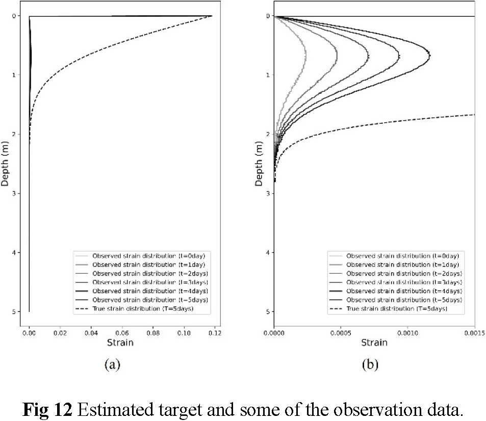
First, in Case 4, the acquisition of the initial conditions is discussed with two-time axes: one demonstrates the loading start time while the other one depicts the observation start time. As shown in Fig. 11, the loading start time is set to T=0 day and the observation of 10 days starts when 5 days have elapsed. Moreover, the observation start time is set to t=0 day; hence, T=5 days and t=0 day correspond to the same day. As shown in Fig. 12, the strain, which indicates the displacement, is zero except at the ground surface at the observation start time. Therefore, the actual strain distribution (“Strain distribution at T=5 days” in Fig. 11 and “True strain distribution” in Fig. 12) is different from the strain distribution observed at the same time (“Strain distribution at t=0 day” in Fig. 11 and “Observation strain distribution (t=0 day) in Fig. 12); similarly, the actual strain is different from the strain observed thereafter. Therefore, in this section1, the strain distributions of 10 days from the start of observation, i.e., 15 days after the start of loading (“Training (Observation) data in Fig. 11), are adopted as the observation data to estimate the actual strain distribution (“Strain at T=5 days” in Fig. 11) the fifth day after the start of loading.

The actual strain distribution estimated by PINN at 5 days after the start of loading is shown in Fig. 13. The standard deviations calculated from these results are shown below each figure. Except for the ground surface, the results are generally accurate, regardless of the noise. The standard deviations are not large, and the dispersion is small. The prediction accuracy of the strain distribution near the ground surface is lower than that near the bottom because the strain changes significantly at the ground surface near the loading area but slightly near the bottom at an early stage of consolidation. As shown in Fig. 11 (“Training (Observation) data” box), the observed data for the first 10 days of observation do not have the same shape as the strain distribution at 5 days after the start of loading (“Estimate” box in Fig. 11), which is the target of the estimation. However, according to the results in Fig. 13, an accurate estimation is possible because the residual of PDE is incorporated in the loss function.

Next, Case 5 discusses the acquisition of boundary conditions using the PINN model learned in Case 3. In this study, a consolidation layer (Fig. 1) is used, in which the drained and undrained conditions, which are known as general conditions, are set at the ground surface (z=0.0 m) and at the bottom (z=5.0 m), respectively. As the drained and undrained conditions are as shown in Eq. 4 and 5, it is possible to determine whether each boundary condition has been obtained by calculating the values of the time derivative of the strain at the ground surface and the spatial derivative of the strain at the bottom.

The calculation results of the time derivative of the strain at the ground surface and the spatial derivative of the strain at the bottom during the first 100 days of loading by PINN are shown in Fig. 14. As the loss at training time in Case 5 is the same as that in Case 3, only the time derivative of the strain at the ground surface ( ∂𝜀⁄∂t ) and the spatial derivative of the strain at the bottom ( ∂𝜀⁄∂z ) are shown as they change with time from the start of loading to 100 days after the start of loading. First, the time derivative of the strain at the ground surface, denoted by the solid line in Fig. 14, is zero immediately after the start of loading and remains close to zero for the next 100 days. The spatial derivative of the strain at the bottom also gradually converges to zero after about 50 days. Because consolidation is incomplete after 100 days from the start of loading, the spatial derivative has not yet completely converged to zero, but it is expected to approach zero as consolidation proceeds. The time derivative of the strain at the ground surface and the spatial derivative at the bottom converge to zero over time, which is consistent with the boundary conditions set when the observation data were generated, indicating that the boundary conditions have been captured.

(5) Prediction results assuming construction site measurement

In this section, training and validation for cases with a set number of measurements and measurement intervals based on actual measurement cases²⁹⁾, ³⁰⁾ are conducted. The training data used are shown in Table 3 and are the same as those used in Case 3, except for the observation data used for training. In Case 5, 1446 observation data were used, with 1 m intervals in the depth direction and one observation per day in the time direction, following a measurement case of previous studies²⁹⁾, ³⁰⁾. The parameters used for training are the same as those used in Cases 1-5, but the number of training epochs is 200.

Fig. 15 shows the validation results for three cases with different noise levels. As in Case 3, these three cases were trained 10 times each in the same manner. The standard deviations calculated based on these results are shown below each figure. In all cases, the standard deviations are slightly larger than those of Case 3, but the differences are not large compared to these cases, and the strain distribution after 100 days from the start of loading is sufficiently predicted. Comparing the three cases in Case 6, Cases 6-0 and 6-1, which contain 0% and 1% noise, respectively, show similar trends, while only Case 6-10, which contains 10% noise, shows a large deviation. For a more accurate prediction, more information should be integrated into the loss function, such as boundary conditions. However, as mentioned above, because the strain distribution is generally captured, prediction is possible even when the number of data is small. In this study, the number of data was set based on past measurement cases, but it is expected that more detailed data will become available with the development of measurement technology, such as optical fibers, and further improvement in accuracy can be expected in the future.

4. CONCLUSIONS

The strain distribution and the amount of settlement due to consolidation were predicted by adopting the PINN, wherein the physical laws are incorporated in the loss function in the NN. In this study, Mikasa’s consolidation equation considered the fundamental physics controlling the phenomena.

It was demonstrated that the long-term strain distribution and the amount of settlement can be predicted with high accuracy even with short observation by the PINN if the period of collocation points covers the entire period up to the prediction date. However, it was difficult to predict them accurately when the coverage of the collocation points evaluating PDE is short. Therefore, it is necessary to not only consider the PDE but also to pay attention to the distribution of the collocation points for training, so that the collocation points are taken from a longer period, including the unobserved period up to the prediction date.

In addition, the predicted strain distributions indicate that the ground surface and the bottom of the clay layer are drained and undrained conditions, respectively. In other words, the NN may have acquired those conditions from the first 10 days of observation and predicted the behavior of the soil after 100 days based on the PDE using the derived conditions. Although many studies on PINN have been conducted in recent years, in the field of civil engineering, which is the subject of this study, there are no examples of estimating the initial and boundary conditions in addition to predicting the strain distribution and settlement due to consolidation, as in this study. When the initial conditions are unknown, the shape of the observed data differs significantly from the actual strain distribution; hence, accurate initial conditions must be obtained to predict displacements. Thus, even when the actual strain distribution is unavailable owing to the difference between the loading and observation start times, the actual strain distribution can be roughly estimated by using this PINN model. This enables the accurate prediction of the strain distribution and displacement at an arbitrary point, even after a certain period of time has elapsed since the start of loading, which is useful in the field. Even when the number of observations and observation intervals actually performed in the field are used as references and the observation data used for learning are reduced to 15% or less, it is possible to predict the strain distribution approximately.

In conclusion, the constructed PINN model is capable of highly accurate prediction and estimation without computationally intensive numerical analysis and many laboratory tests, even in the presence of unknown parameters and uncertainties, which are challenges in ground consolidation problems. Furthermore, considering the capabilities of the constructed PINN model in estimating the initial and boundary conditions, the application of PINN to inverse problems will be explored in future research. Furthermore, this is expected to lead to a reduction in computationally expensive numerical analyses and numerous laboratory tests that were previously required, while maintaining the prediction and estimation accuracy of consolidation phenomena. In this study, the exact solution obtained by the FTCS method was compared with the predictions by the PINN model. In the future, comparisons with results from other models, such as FEM, will be considered. In addition, similar prediction and estimation using actual measurements will be conducted, as this study uses values calculated by the FTCS method as observed data to examine the applicability of the PINN model.

Furthermore, our research extends beyond consolidation problems to encompass other critical areas in geotechnical and civil engineering, such as slope stability analysis^31)-35) and the prediction of three-dimensional bridge deterioration^36)-40). We anticipate that integrating mechanistic principles, analogous to the physics-informed approach employed in this study, into these diverse fields will not only broaden the scope of application but also significantly enhance predictive accuracy. Exploring these extensions constitutes a key direction for our future work.

Acknowledgments

This work was supported by JST [Moonshot Research and Development], CSTI [Cross-Ministerial Strategic Innovation Promotion Program (SIP), the 3rd period of SIP “Smart Infrastructure Management System” Grant Number JPJ012187] and JSPS KAKENHI Grant Number [JPMJMS2032, 23H00198, 23K22831].

References

• 1)  Mizuno, K., Watanabe, Y., Kobayashi, M., Noguchi, T., Aoki, Y., Yamamoto, T. and Takahashi, M.: Long-Term consolidation settlement prediction of D-Runway in Tokyo International Airport, Journal of the Society of Materials Science, Japan, Vol. 61, No. 1, pp. 78-84, DOI: doi.org/10.2472/jsms.61.78, 2012. (in Japanese)
• 2)  Noguchi, T., Watabe, Y., Suzuki, H., Sakaiya, T., Kakehashi, K., Ogura, K. and Mizuno, K.: Design of D-Runway in Haneda Airport, Journal of Japan Society of Civil Engineers, Ser. C (Geosphere Engineering), Vol. 68, Issue 1, pp. 150-162, DOI: doi.org/10.2208/jscejge.68.150, 2012. (in Japanese)
• 3)  Noguchi, T., Tanaka, M., Watabe, Y., Sakajo, S. and Sadamura, T.: Verification of 3-D visualization of ground at Tokyo International Airport, Japanese Geotechnical Journal, Vol. 6, Issue 1, pp. 69-79, DOI: doi.org/10.3208/jgs.6.69, 2011. (in Japanese)
• 4)  Asaoka, A.: Observational procedure of settlement prediction, Soils and Foundations, Vol. 18, Issue 4, pp. 87-101, DOI: doi.org/10.3208/sandf1972.18.4_87, 1978.
• 5)  Singh, V., Bano, S., Yadav, A. K. and Ahmad, S.: Feasibility of artificial neural network in civil engineering, International Journal of Trend in Scientific Research and Development, Vo. 3, Issue 3, pp. 724-728, DOI: doi.org/10.31142/ijtsrd22985, 2019.
• 6)  Nejad, F. O., Jaksa, M. B., Kakhi, M. and McCabe, B. A., Prediction of pile settlement using artificial neural networks based on standard penetration test data, Computers and Geotechnics, Vol. 36, Issue 7, pp. 1125-1133, DOI: doi.org/10.1016/j.compgeo.2009.04.003, 2009.
• 7)  Shahin, M., Maier, H. R. and Jaksa, M. B.: Predicting settlement of shallow foundations using neural networks, Journal of Geotechnical and Geoenvironmental Engineering, No. 128, Issue 9, pp. 785-793, DOI: doi.org/10.1061/(ASCE)1090-0241(2002)128:9(785), 2002.
• 8)  Kanayama, M., Rohe, A. and Paassen, L. A., Using and improving neural network models for Ground Settlement Prediction, Geotechnical and Geological Engineering, No. 32, pp. 687-697, DOI: doi.org/10.1007/s10706-014-9745-8, 2014.
• 9)  Kurnaz, T. F., Dagdeviren, U., Yildiz, M. and Ozkan, O.: Prediction of compressibility parameters of the soils using artificial neural network, SpringerPlus, No. 5, 1801, 11p, DOI: doi.org/10.1186/s40064-016-3494-5, 2016.
• 10)  Park, H. I. and Lee, S. R.: Evaluation of the compression index of soils using an artificial neural network, Computers and Geotechnics, Vol. 38, Issue 4, pp. 472-481, DOI: doi.org/10.1016/j.compgeo.2011.02.011, 2011.
• 11)  Pham, B. T., Nguyen, M. D., Bui, K. T, Prakash, I., Chapi, K. and Bui, D. T.: A novel artificial intelligence approach based on multi-layer perceptron neural network and biogeography-based optimization for predicting coefficient of consolidation of soil, CATENA, Vol. 173, pp. 302-311, DOI: doi.org/10.1016/j.catena.2018.10.004, 2019.
• 12)  Oda, K., Yokoyama, K. and Bu, L. D.: Prediction of compressibility parameters of the soils using artificial neural network, Prediction of compressibility parameters of the soils using artificial neural network, Vol. 2, Issue 74, pp. 2529-2534, DOI: doi.org/10.1186/s40064-016-3494-5, 2016.
• 13)  Deguang, M., Tianzhi, Z., Bingxin, L. and Yanying, D.: Research for settlement prediction on the based of neural network and ADINA, 2009 International Forum on Computer Science-Technology and Applications, pp. 123-126, DOI: 10.1109/IFCSTA.2009.269, 2009.
• 14)  Kingston, G. B., Maier, H.R. and Lambert, M.F.: Calibration and validation of neural networks to ensure physically plausible hydrological modeling, Journal of Hydrology, Vol. 314, No.1, pp. 158-176, DOI: doi.org/10.1016/j.jhydrol.2005.03.013, 2005.
• 15)  Raissi, M., Perdikaris, P. and Karniadakis, G.E.: Physics-informed neural networks: A deep learning framework for solving forward and inverse problems involving nonlinear partial differential equations, Journal of Computational Physics, 378, pp. 686-707, DOI: doi.org/10.1016/j.jcp.2018.10.045, 2019.
• 16)  Yang, Q., Wang, Z., Guo, K., Cai, C. and Qu, X.:Physics-driven Synthetic Data Learning for Biomedical Magnetic Resonance, IEEE Signal Processing Magazine, DOI: doi.org/10.48550/arXiv.2203.11178, 2022.
• 17)  Joo, J. and Moon, H.: Quantum variational PDE solver with machine learning, Quantum Physics, DOI: doi.org/10. 48550/arXiv.2109.09216, 2021.
• 18)  Samaniego, E., Anitescu, C., Goswami, S., Nguyen-Thanh, V.M., Guo, H., Hamdia, K., Zhuang, X. and Rabczuk, T.: An energy approach to the solution of partial differential equations in computational mechanics via machine learning: Concepts, implementation and applications, Computer Methods in Applied Mechanics and Engineering, 362, 112790, DOI: doi.org/10.1016/j.cma.2019.112790, 2020.
• 19)  Zhu, Q., Liu, Z. and Yan, J.: Machine learning for metal additive manufacturing: predicting temperature and melt pool fluid dynamics using physics-informed neural networks, Computational Mechanics, 67, pp. 619-635, DOI: doi.org/10.1007/s00466-020-01952-9, 2021.
• 20)  Arthurs, C. and King, A. P.: Active training of physics-informed neural networks to aggregate and interpolate parametric solutions to the Navier-Stokes equations, Journal of Computational Physics, Vol. 438, 110364, 17p, DOI: doi.org/10.1016/j.jcp.2021.110364, 2021.
• 21)  Mao, Z., Jagtap, A. and Karniadakis, G.: Physics-informed neural networks for high-speed flows, Computer Methods in Applied Mechanics and Engineering, Vol. 360, No. 1, 112789, DOI: doi.org/10.1016/j.cma.2019.112789, 2019.
• 22)  Lu, Y. and Mei, G., A Deep Learning Approach for Predicting Two-Dimensional Soil Consolidation Using Physics-Informed Neural Networks (PINN), Mathematics, Vol. 10, Issue. 16, 2949, DOI: doi.org/10.3390/math10162949, 2022.
• 23)  Zhang, S., Lan, P., Li, H.C., Tong, C. X. and Sheng, D., Physics-informed neural networks for consolidation of soils, Engineering Computations, Vol. 39, Issue 7, pp. 2845-2865, DOI: doi.org/10.1108/EC-08-2021-0492, 2022.
• 24)  Wang, Y., Shi, C., Shi, J. and Lu, H., Data-driven forward and inverse analysis of two-dimensional soil consolidation using physics-informed neural network, Acta Geotechnica, Vol. 19, pp. 8051-8069, DOI: doi.org/10.1007/s11440-024-02345-5, 2024.
• 25)  Chang, L. J., Mo, Y. F., Ling, L. M. and Zeng, D. L.: Data-driven parity-time-symmetric vector rogue wave solutions of multi-component nonlinear Schrödinger equation, Chinese Physics B, Vol. 31, No. 6, 060201, DOI: 10.1088/1674-1056/ac4cc5, 2022.
• 26)  Nakano, M., Katagiri, S. and Okuno, M., Development of PE-Pipe Optical Fiber Sensor for Observation of Ground Deformation, Journal of Applied Computing in Civil Engineering, Vol. 17, pp.83-90, DOI: doi.org/10.2208/journalac2003.17.0_83, 2008. (in Japanese)
• 27)  Yashima, A., Tsuji, S., Yoshida, K. and Yokota, Y., A new optical fiber sensor to assess the stability of geogrid reinforced soil walls, Geosynthetics International, Vol. 16, Issue 4, pp. 238-245, DOI: doi.org/10.1680/gein.2009.16.4.238, 2015
• 28)  Ngo, S. I. and Lim, Y. I.: Solution and Parameter Identification of a Fixed-Bed Reactor Model for Catalytic CO2 Methanation Using Physics-Informed Neural Networks, catalysts, 11, 1304, DOI: 10.3390/catal11111304, 2021.
• 29)  Takahama, T., Sakata, S., Hirota, T., Yokotani, A. and Kurosawa, K.: Development of Multi-level Inclinometer using Optical Fiber Bragg Gratings - Experimental results of system performance and field tests -, Japanese Geotechnical Journal, Vol. 1, Issue 3, pp. 95-103, DOI: doi.org/10.3208/jgs.1.95, 2006. (in Japanese)
• 30)  Chapeleau, X., Drissi-habti, M. and Tomiyama, T.: Embedded Optical Fiber Sensors for In Situ and Continuous Health Monitoring of Composite Materials in Civil Engineering Structures, Journal of the Japan Society for Composite Materials, Vol. 36, Issue 1, pp.25-30, DOI: doi.org/10.6089/jscm.36.25, 2010. (in Japanese)
• 31)  Areerob, K., Nguyen, V. Q., Li, X., Inadomi, S., Shimada, T., Kanasaki, H., Wang, Z., Suganuma, M., Chun, P.J., and Okatani, T. (2025). Multimodal artificial intelligence approaches using large language models for expert‐level landslide image analysis. Computer‐Aided Civil and Infrastructure Engineering.
• 32)  Opara, J. N., and Moriwaki, R. (2024). Delineating landslide and debris flow detection in Japan through aerial photography: A YOLO v8 approach to disaster management. Intelligence, Informatics and Infrastructure, 5(1), 111-123.
• 33)  Li, X., Nishio, M., Sugawara, K., Iwanaga, S., and Chun, P. J. (2023). Surrogate Model Development for Slope Stability Analysis Using Machine Learning. Sustainability, 15(14), 10793.
• 34)  Opara, J. N., Moriwaki, R., and Chun, P. J. (2023). Automated Landslide Mapping in Japan using the Segformer Model: Enhancing Accuracy and Efficiency in Disaster Management. Intelligence, Informatics and Infrastructure, 4(2), 75-86.
• 35)  Li, X., Nishio, M., Sugawara, K., Iwanaga, S., Shimada, T., Kanasaki, H., Kanai, H., Zheng, S. and Chun, P. J. (2024). Enhancing prediction of landslide dam stability through AI models: A comparative study with traditional approaches. Geomorphology, 454, 109120.
• 36)  Lin, C., Abe, S., Zheng, S., Li, X., and Chun, P. J. (2025). A structure‐oriented loss function for automated semantic segmentation of bridge point clouds. Computer-Aided Civil and Infrastructure Engineering, 40(6), 801-816.
• 37)  Yamashita, M., Kawanishi, K., Hashizume, K., and Chun, P. J. (2024). Infrared thermography and 3D pavement surface unevenness measurement algorithm for damage assessment of concrete bridge decks. Computer‐Aided Civil and Infrastructure Engineering.
• 38)  Chun, P. J., and Kikuta, T. (2024). Self‐training with Bayesian neural networks and spatial priors for unsupervised domain adaptation in crack segmentation. Computer‐Aided Civil and Infrastructure Engineering, 39(17), 2642-2661.
• 39)  Hattori, K., Oki, K., Sugita, A., Sugiyama, T., and Chun, P. J. (2024). Deep learning-based corrosion inspection of longspan bridges with BIM integration. Heliyon, 10(15).
• 40)  Inadomi, S. and Chun, P. J. (2025). Spatially-Aware Deterioration Prediction of Bridges Using a Graph Transformer and Inspection Data. Computer-Aided Civil and Infrastructure Engineering (in print)