Abstract
An accurate prediction of pavement condition is essential for effective pavement management systems, enabling road agencies to optimize maintenance strategies and extend the service life of road networks. The Pavement Condition Index (PCI) is one of the most commonly used pavement health indicators for assessing pavement deterioration. However, in many predictive models, PCI is often converted into an ordinal variable, which can result in the loss of valuable information regarding gradual deterioration patterns. This study aims to develop predictive pavement deterioration models treating PCI as a continuous variable to better capture the gradual deterioration of pavements over time. Both statistical and machine learning models were explored, including multiple regression, decision tree, random forest, and Artificial Neural Networks (ANN). Hyperparameter tuning was performed to optimize the performance of machine learning models, ensuring a balance between underfitting and overfitting. The models were evaluated based on R2 and Root Mean Square Error (RMSE) values for both training and testing datasets, with performance parameters compared to identify the most effective model for predicting PCI as a continuous value. The findings indicate that random forest and double-layer ANN models possess superior predictive accuracy and generalization capabilities compared to other approaches, particularly in capturing complex deterioration patterns over time. The practical applicability of treating PCI as a continuous variable was explored, showing that it allows road agencies to identify critical deterioration stages and plan timely preventive maintenance and rehabilitation measures.
1. INTRODUCTION
(1) Background
Asphalt pavements are essential components of transportation networks, providing critical links for communication and logistics. These pavements are composed of various natural resources that degrade over time due to extrinsic factors such as traffic loads and environmental conditions1,2). Maintaining pavements in good condition thus require regular inspections for the implementation of appropriate maintenance strategies based on pavement condition assessments.
In pavement engineering, several indices are used to evaluate pavement condition, including the Pavement Condition Index (PCI), International Roughness Index (IRI), Structural Number (SN), and Present Serviceability Rating (PSR)3). Among these, PCI and IRI are the most widely adopted indices due to their relevance in assessing surface distresses and road smoothness, respectively4,5). The PCI measures the overall condition of a pavement on a scale ranging from 0 to 100 by analyzing various pavement distresses such as cracks, potholes, and rutting (ASTM D6433-20)6). In contrast, the IRI quantifies pavement roughness, expressed in meters per kilometer (m/km), representing the ride quality experienced by road users (ASTM E1926-08)7). Road agencies may choose different indices based on their pavement management objectives. PCI is more relevant for evaluating surface distresses and identifying maintenance needs, while IRI is commonly used to assess road smoothness and driving comfort, typically measured using specialized instruments such as profilometers.
The PCI is widely used in pavement management due to its ease of data collection, as it does not require specialized devices. However, after data collection, PCI is often converted into ordinal variables for pavement deterioration prediction models, with classifications such as “Poor,” “Fair,” and “Very Good.” Many pavement engineers categorize PCI into different ranges to associate them with specific maintenance activities. For example, Kheirati et al. (2022) classified PCI into three ranges: Class 1 (70-100), Class 2 (55-70), and Class 3 (0-55), and predicted pavement condition over time considering factors such as structural adequacy, pavement roughness, road safety, and surface distress using an Artificial Neural Network (ANN) model8). Similarly, Piryonesi et al., 2021 categorized PCI into five ordinal levels and developed a pavement condition prediction model based on factors such as location, temperature, traffic volume, freeze index, freeze- thaw cycles, functional class, and precipitation9). In a previous study, Amir et al. (2023) developed a pavement condition prediction model for the provincial highway network of Pakistan by classifying PCI into three categories - Good (71- 100), Fair (51-70), and Poor (0-50) - aligning this classification with the three types of maintenance strategies used by the associated road agency5).
While most existing studies rely on categorical PCI models, fewer studies have explored prediction models that treat PCI as a continuous variable. Ali et al. (2022) developed a fuzzy logic-based system for predicting pavement condition by treating PCI as a continuous variable and utilizing pavement distress data from the United States and Canada10). Similarly, other studies have focused on predicting pavement condition using distress types and severity through machine learning algorithms11,12). A limited number of studies have used extrinsic factors to predict PCI as a continuous variable. For instance, Sidess et al. (2012) presented a pavement condition prediction model that treated PCI as a continuous value, incorporating factors such as structural number, asphalt layer thickness, subgrade strength, and environmental conditions13). Radwan et al. (2024) developed a modeling approach that predicted PCI as a function of pavement age14). Similarly, a study by Younos et al. (2020) investigated pavement performance based on the combined effects of climate and traffic loading, using PCI as the pavement performance index. However, pavement deterioration is influenced by multiple factors beyond climatic conditions and traffic loading. These include pavement design, the condition of road-associated structures, traffic volume, and roadside land use, whether the area is open or built-up. The roadside environment also plays a critical role in water infiltration, which can be detrimental to the road structure. Therefore, a pavement condition prediction model should incorporate a comprehensive set of factors to support efficient maintenance planning.
In addition, developing a model that treats PCI as a continuous variable better reflects the gradual deterioration of pavement over time rather than grouping conditions into broad categories, which can lead to information loss. Once PCI is converted into a categorical variable, it becomes challenging for maintenance agencies to determine the exact time period when pavement condition begins to degrade. For example, in previous studies by the authors15), and in other studies16,17), deterioration trends based on categorical PCI models exhibit abrupt changes in condition states, shifting from one category to another without capturing the gradual degradation process. In contrast, treating PCI as a continuous variable enables agencies to predict, with greater accuracy, the point in a pavement’s life cycle when deterioration actually begins. This allows for timely maintenance interventions, which are crucial in extending the pavement’s service life.
(2) Research gap
Existing studies on pavement condition prediction models that incorporate extrinsic factors often either treat PCI as a categorical variable or are constrained by a limited range of predictive factors. Most studies primarily focus on distress-related variables or a narrow subset of structural and environmental conditions, limiting their applicability in capturing the full complexity of pavement deterioration. Since pavement deterioration is influenced by a complex interplay of structural, environmental, and operational factors, failing to incorporate a broader set of variables can reduce the predictive accuracy of existing models. Therefore, there is a need to develop and evaluate various statistical and machine-learning approaches to identify the most effective method for predicting pavement condition using PCI as a continuous variable.
(3) Research objectives and contributions
This research aims to address the identified gaps by exploring various analytical techniques to predict pavement condition and identify the most effective model that considers PCI as a continuous variable. The study utilizes data from the provincial highway network of Pakistan and incorporates a wide range of extrinsic factors, including age, traffic volume, drainage condition, traffic loading, paved shoulder, unpaved shoulder, built-up area, open area, climate, drainage presence, culverts, tourism roads, mines roads, and asphalt concrete base course (ACBC) layer thickness. The statistical and machine learning algorithms, such as multiple regression, decision trees, random forest, and ANN, were applied, and their performance was evaluated. The best models were then used to demonstrate the practical advantages of treating PCI as a continuous variable in real-world pavement management scenarios.
Hence, the study contributes to the literature by addressing three key gaps. First, it addresses the use of PCI as a continuous variable for predicting pavement condition using extrinsic factors, whereas most previous studies have primarily focused on the association between PCI (as a continuous variable) and distress types or severity. Second, this study incorporates a wider range of extrinsic factors compared to previous research, which typically used only a limited number of factors. Third, the study explicitly defines and highlights the practical advantages of using continuous PCI models for preventive and rehabilitation maintenance planning.
2. DATASET
This study utilized data on the provincial highways of Khyber Pakhtunkhwa province, Pakistan. Khyber Pakhtunkhwa is located in the northern part of Pakistan, and is famous for tourism, agriculture, forestry, and mining. The provincial highway network of Khyber Pakhtunkhwa is more than 3,000 kilometers in length and spans a diversity of geographic and climatic conditions. The plain areas in the south and center divisions tend to have hot summers and mild winters, whereas the mountainous regions in the south, east, and north divisions experience harsh winters with heavy snowfall and relatively cool summers. Provincial roads thus play an important role in supporting socio-economic activities but are also exposed to a variety of severe environmental and mechanical loadings.
Data on the provincial roads were gathered by field survey in 200 m-long sections. Due to practical and financial limitations, a stratified sampling approach was adopted to facilitate the investigation of a representative sample of the entire highway network. The sampling considered three different factors: pavement age, climatic conditions, and geographic location. The minimum required number of samples of these road segments (n) for a 3,000 km road network was calculated using Equation (i)18).
Where:
n = required sample size (number of kilometers of road network to be surveyed)
z = z-score corresponding to the desired confidence level (CI) (1.96 corresponding to 95% CI).
p = estimated population proportion (0.5, assuming maximum variability which is conservative estimate often used when the true proportion is unknown).
e = margin of error (6%)
N = total population size (3,000 kilometers of high- way network)
A sample size of 241 km (1209 sections) was chosen, as this was both feasible considering the research budget and represented a 95% confidence interval and 6% margin of error for the 3,000 km network19). The distribution of the surveyed roads is shown in Fig.1. The field survey gathered data on the presence of ten different pavement distresses in each road section and their area and level of severity. These distress data were used to calculate the pavement condition numerical value ranging from 0 to 100 that captures the index (PCI) for each section as specified by the Distress Identification Manual5). The process of PCI calculation involves determining the PCI for each 200-meter road section by first identifying and quantifying the extent and severity of all observed distress types. The distress density for each distress type is calculated by dividing its total quantity by the total area of the 200-meter pavement section. Each distress type is then assigned a deduct value based on its severity level (low, medium, or high) using the deduct value curve from ASTM D6433-2020). These values are used to compute the total deduct value (TDV) for the section. An adjustment is applied to the total deduct value using CDV-TDV adjustment curves to ensure the final PCI value falls within the 0-100 range. The maximum corrected deduct value (maxCDV) is then used to calculate the PCI using Equation (ii):


The PCI score for each 200-meter section is obtained by subtracting the maxCDV from 100. A higher PCI indicates better pavement condition, while a lower PCI suggests poor condition. In this study, PCI is treated as continuous and serves as the dependent variable for the analysis.
In addition to the pavement condition, data were also gathered on the features of each road section, such as pavement design, road characteristics, and climatic conditions. In total, 16 features were adopted as independent variables for the pavement deterioration modeling, with their details provided in Table 1. The selection of these independent variables was based on a comprehensive review of relevant literature and guidelines, including AASHTO standards21). These features were chosen to ensure a broad representation of factors that could influence pavement condition. Then these variables were coded based on their appropriateness for the proposed analysis. The detail of the data coding used for analysis is also shown in Table 1. The statistics description of data is shown in Fig.2a and 2b.
3. ANALYSIS METHODOLOGY
Deterioration modeling for provincial highways in Khyber Pakhtunkhwa was explored using five statistical and machine learning-based regression techniques. Fig.3 illustrates the methodology flow chart of the research, where different shapes are used to represent various components of the process. Rectangles denote the key steps involved in pavement condition prediction, including data collection, data preparation, model selection, validation, and evaluation. Rounded rectangles highlight critical decision-making stages, such as model selection and its application in maintenance management. Parallelograms are used to classify variables, distinguishing between independent variables (extrinsic factors) and dependent variables (PCI calculations). Additionally, different colored lines are used to enhance clarity in methodology flow. Black solid lines represent the primary flow of the process, showing how data progresses from collection to model evaluation and practical application. Blue arrows highlight three main stages of research: first, the identification and classification of dependent and independent variables, which include extrinsic factors and distress data; second, the modeling process, which involves data preparation, model selection, hyperparameter tuning, and validation; and third, the model evaluation and application, where model performance is assessed using R2 and RMSE, and the predicted PCI values are analyzed for maintenance planning.

The dependent variable was the PCI as continuous data, and the independent variables were the 16 road features shown in Table 1. First, the 1209 road sections were randomly split 7:3 - 70% for model training and 30% for model validation. The prediction capability of each of the models was checked using two metrics: the coefficient of determination (R2) and the root mean square error (RMSE). Both R2 and RMSE are important performance metrics to consider. R2 indicates the proportion of variance in the dependent variable (PCI) that is predictable from the independent variables (road-related factors), with a higher value reflecting better model fit. The focus in predictive modeling is often on the Test R2, which measures how well the model generalizes to unseen data. A high-Test R2 signifies that the model captures meaningful patterns rather than noise from the training data, making it reliable for real-world applications. RMSE, on the other hand, measures the average magnitude of prediction errors, with lower values indicating more accurate predictions. In practical applications, Test RMSE is more critical than Train RMSE, as it provides insights into how far off the model’s predictions are for unseen data. The details of the four algorithms are as follows.
(1) Multiple regression model
A statistical technique, multiple regression analysis, was first applied to model the relationship between PCI as the dependent variable and other extrinsic road-related factors as independent variables (Table 1). The general form of the multiple regression equation used in this analysis is:
Where:
y = dependent variable (PCI),
ω0 = intercept term,
xn = independent variables (road factors),
ωn = regression coefficients for each independent variable.
The regression coefficients indicate the contribution of each independent variable to the predicted PCI value. The analysis was conducted using scikit-learn library in Python, which provides tools for building and evaluating regression models23).
(2) Decision tree model
A second predictive model was developed using decision tree analysis, a machine learning algorithm based on the Classification and Regression Tree (CART) framework. The CART algorithm, introduced by Breiman et al. (1984), constructs a binary regression tree by recursively splitting the dataset into two groups at each decision node, based on a feature that minimizes the Mean Squared Error (MSE) of the target variable in the resulting nodes22). To ensure that the model was neither underfitting nor overfitting the data, the tree depth parameter was varied between 1 and 20, The decisiontreeregressor from the scikit-learn and the model’s performance was evaluated using the R2 and RMSE metrics23). The optimal tree depth was identified based on the highest R2 score and lowest RMSE on the test set, ensuring the model’s balance between accuracy and generalizability.
(3) Random forest regression model
A third predictive model was developed using the random forest algorithm, a machine learning technique that builds an ensemble of decision trees to improve prediction accuracy and reduce the risk of overfitting. The random forest algorithm, introduced by Breiman (2001), operates by constructing multiple decision trees during training and outputting the average prediction of the individual trees for regression tasks22). The random forest regressor, implemented using the RandomForestRegressor from the scikit-learn library, was used for PCI prediction model23). To optimize the model’s performance, hyperparameter tuning was performed by varying the maximum tree depth between 1 and 20. The optimal model was selected based on the highest R2 score and lowest RMSE on the test set.
(4) Artificial neural network model
A fourth predictive model was developed using an Artificial Neural Network (ANN), a widely used machine learning technique that is similar to the structure and function of biological neural networks to identify complex patterns in data24). The ANN models were implemented using the MLPRegressor class from the scikit-learn library in Python to develop the PCI prediction model23). Two types of ANN models were developed: a single-layer model and a double-layer model. For the single-layer ANN, hyperparameter tuning was performed by varying the number of nodes in the hidden layer from 1 to 16, to identify the best-performing model based on R2 and RMSE metrics on both the training and test sets.
For the double-layer ANN, a randomized search approach was applied to perform hyperparameter tuning. The randomized search approach, introduced by Bergstra and Bengio (2012)25), is an efficient method for hyperparameter tuning in machine learning models. Unlike Grid search approach, which thoroughly evaluates all possible parameter combinations, it randomly samples a specified number of parameter settings from a defined distribution. This method significantly reduces computational time while also covering a broad range of hyperparameter values, making it particularly useful for complex models like ANN26). The randomized search method explored hyperparameter space to identify the optimal configuration of nodes in each layer that yielded the best R2 score.
4. RESULTS AND DISCUSSION
(1) Details of prediction models
a) Multiple regression model
Table 2 presents the regression coefficients for each variable used in the multiple regression model. PCI was predicted by applying these coefficients along with the intercept value in Equation (1). The intercept value of 65.2207 represents the baseline PCI when all predictor variables are zero, whereas the coefficients indicate the impact of each variable on the predicted PCI. For instance, the coefficient for age implies that PCI decreases by approximately 7.99 units for each additional year of service.

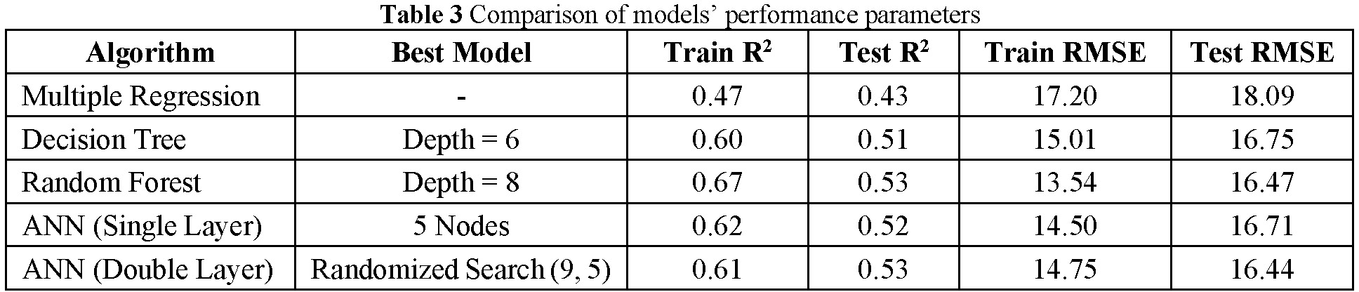
Table 3 shows the performance evaluation metrics for the multiple regression model. The R2 value of 0.47 for the training set and 0.43 for testing set indicates that the model explains approximately 47% of the variance in the training data and 43% in the testing data. This suggests that the model captures a moderate proportion of the variability in PCI but leaves some unexplained variance, possibly due to additional unmeasured factors. The RMSE values of 17.20 for the training set and 18.09 for the testing set represent the average error in PCI predictions. These RMSE values indicate that, on average, the model’s predictions deviate from the actual PCI values by approximately 17 to 18 units.
b) Decision tree model
For the decision tree model, hyperparameter tuning was performed by varying the maximum tree depth from 1 to 20, as illustrated in Fig.4a, to identify the optimal depth for achieving the best predictive performance. It was observed that the R2 values for the training set increase as the tree depth increases, reaching 0.72 at a depth of 12 or higher, indicating that the model fits the training data well at higher depths. However, the test R2 values peak at a depth of 6, with a value of 0.51, after which the performance slightly decreases as the tree becomes more complex as seen in Fig.4a. This suggests that the model starts to overfit the training data at depths beyond 6, as it captures noise and specific patterns that do not generalize well to unseen data. Similarly, the RMSE values for the training set decrease as the tree depth increases, showing that the model is minimizing the error for the training data. However, the test RMSE values reach their minimum of 16.75 at a depth of 6, after which the error starts to increase, indicating that the model’s predictions on the test set become less accurate beyond this point. Based on the performance evaluation, a maximum depth of 6 was selected as the optimal depth for the decision tree prediction model, balancing both R2 and RMSE values for the training and testing datasets.

c) Random forest regression model
For the random forest model, hyperparameter tuning was conducted by varying the maximum tree depth from 1 to 20, as shown in Fig.4b, to determine the optimal depth for achieving the best predictive performance. The R2 values for the training set increase with an increase of tree depth, reaching a maximum of 0.71 at a depth of 15. This indicates that the model can fit the training data better as the tree depth increases. However, similar to the decision tree model, the test R2 value reached its maximum at a depth of 8, with a value of 0.53, after which it flattened. This suggests that deeper trees do not significantly improve the model’s ability to generalize to unseen data beyond a certain point. The RMSE values for the training set decrease consistently as the tree depth increases, indicating that the model is reducing the prediction error for the training data. The test RMSE values, however, reach their minimum of 16.47 at a depth of 8, after which the error remains relatively stable. This stability suggests that increasing the depth beyond 8 does not necessarily lead to overfitting, as seen in simpler decision tree models, due to the averaging process in the random forest algorithm. Based on this performance evaluation, a tree depth of 8 was selected as the optimal depth for the random forest prediction model.
d) Artificial neural network model
Two ANN models were developed to predict the PCI: a single-layer model with varying numbers of nodes and a double-layer model using a randomized search approach for hyperparameter tuning. For the single-layer ANN model, as shown in Fig.4c, hyperparameter tuning was performed by varying the number of nodes in the hidden layer from 1 to 16. It can be observed that the training R2 value increases with the number of nodes in the hidden layer, indicating that the model learns the patterns in the data more effectively with more nodes. The training R2 stabilizes around 0.66 after 10 nodes, while the test R2 reaches a peak value of 0.51 at 5 nodes. Similarly, the RMSE values for the training set decrease as the number of nodes increases, but the test RMSE shows an optimal point at 5 nodes, with a value of 16.71. Beyond this point, the model starts to slightly overfit the training data.
For the double-layer ANN model, Fig.4d shows the result of the randomized search approach. The hidden layer sizes were varied from (1, 1) to (16, 16), and the corresponding R2 scores were recorded. The randomized search approach optimized the model based on R2 because it is a key metric for evaluating how well the model explains the variance in the target variable (PCI) during hyperparameter tuning. R2 was chosen as the optimization criterion since it reflects the model’s generalization capability and helps avoid overfitting or underfitting during the search process18). In contrast, RMSE is typically used after the hyperparameter tuning phase to evaluate the model’s practical prediction accuracy. Hence, in the randomized search process, R2 was considered only to find the best-performing model. During model training, the sudden drops in R2 scores at nodes (6, 14), (2, 14), (1, 13), and (3, 12) hidden layer sizes were observed which are likely due to a combination of factors, including unstable learning dynamics, weight initialization issues, and overfitting effects. These results reinforce the importance of hyperparameter tuning in ensuring stable and effective training of ANN models. While other factors, such as dataset distribution and initialization randomness, may also contribute to performance fluctuations, a detailed investigation into these aspects was beyond the scope of this study. Future research could further explore how dataset characteristics and model initialization influence hyperparameter tuning effectiveness. The best configuration identified by the randomized search approach was a hidden layer size of (9,5), with a corresponding R2 score of 0.53.
When comparing the single-layer and double- layer models, the double-layer model slightly outperforms the single-layer model, with a higher R2 score on the test set. This indicates that the double-layer architecture provides more flexibility and capability to capture complex relationships in the dataset. However, it should be noted that increasing model complexity can lead to overfitting, which was carefully monitored during the tuning process.
(2) Comparison of models’ performance
A visual comparison of the best models selected from various algorithms is shown in Fig.5. It can be observed that the random forest model and ANN model have the same Test R2 of 0.53, while Test RMSE of 16.47 for the random forest model and Test RMSE of 16.44 for ANN (Double layer) model. These almost identical performance metrics indicate that both models are among the best-performing algorithms for predicting PCI and are capable of capturing the complex relationships between road- related factors and PCI. The decision tree model, with a Test R2 of 0.51 and a Test RMSE of 16.75, also has a very similar performance to Random Forest and ANN models, showing that the model can also be used for predicting PCI. Despite its simplicity and interpretability, the multiple regression model yielded the lowest Test R2 of 0.43 and the highest Test RMSE of 18.09, indicating that it captured only about 43% of the variance in PCI for unseen data.
(3) Comparison of time-dependent deterioration
To evaluate the impact of performance metrics on the prediction of PCI, the above best models were utilized to predict PCI with age (year 1 to year 6). Hence, for comparison purpose, all other variables were kept constant. The variables combination, as shown in Table 4, was chosen to represent common or typical road conditions from the dataset for predicting PCI. The details of the variables used in prediction models are shown in Table 4.

Fig.6 shows the PCI prediction curves for the best-selected models across different age intervals (from 1 year to 6 years) for tourism roads. The graph highlights distinct differences in prediction trends among the models, illustrating the impact of model complexity and generalization capabilities on PCI predictions. From Fig.6, it was observed that the multiple regression model shows a gradual, linear decline in PCI values over time. This behavior occurs because the model applies a linear equation using the regression coefficients derived from the training data. However, the model’s prediction starts at PCI = 72.41 in year 1, based on the fixed input variables. This starting value may result from the fact that the linear model cannot capture complex, non-linear interactions between variables. Instead, it simply multiplies each input variable by its respective coefficient and adds the intercept value, leading to an initial PCI prediction of 72.41. This reflects the model’s simplicity, assuming a constant rate of deterioration as the road ages. The decision tree model displays a stepwise prediction pattern, starting with a PCI value of approximately 75 in year 1, which can be due to the reason that the model predicts the average PCI value within the corresponding split of the training data and the majority of the training data points for similar road sections at Year 1 had PCI values around 75. However, the PCI drops to 65 in year 2, remains stable from year 2 to year 5, and then sharply declines to 20 in year 6. This behavior is characteristic of decision trees, where predictions are based on discrete splits in the data rather than continuous changes. The stepwise nature of these predictions suggests that the model may not fully capture the continuous nature of pavement deterioration. Additionally, this behavior could also be influenced by the limited number of data points available at each split in the decision tree. Since the prediction was based on a fixed set of input variables, the data may lack sufficient variability to allow the model to realize more granular splits, resulting in stepwise predictions instead of a smooth deterioration trend.

Similar to the multiple regression and decision tree models, the random forest model also starts with a lower PCI value of around 69. This is because the random forest prediction is based on averaging the outputs from multiple decision trees. Since the decision tree model starts with a PCI value near 75, the averaging process across different trees in the random forest may bring the starting PCI value closer to 75 (69). The random forest model then exhibits a smooth, non-linear decline in PCI values over time. The model predicts a gradual decrease in PCI from year 1 to year 2, followed by a relatively stable period between years 2 and 4, where the deterioration rate appears to slow down. However, a noticeable decline in PCI is observed between years 4 and 5, with a steeper drop occurring at year 6, indicating accelerated deterioration in later years.
The final model developed from the ANN (Double Layer) demonstrates the most distinct prediction trend, starting with the maximum initial PCI value of 100, indicating that most roads were in good condition at 1 year of age. This can be attributed to the fact that ANN algorithms are designed to capture complex, non-linear interactions between variables, which allows the model to interpret the fixed input variables as a combination, resulting in a perfect PCI value at the start. However, as seen in Fig.6, the overall pattern of the ANN curve shows a gradual decline in PCI from year 1 to year 6, with slightly slower deterioration between years 1 to 2 and 5 to 6, and a nearly constant deterioration rate between years 2 and 5. This pattern indicates that the ANN model is highly sensitive to changes in the input variables, particularly age-related deterioration.
Comparatively, the multiple regression, decision tree, and random forest models do not start at a PCI value of 100 because they rely on rule-based or linear prediction approaches, which are less adaptable in capturing complex interactions. These models generate predictions based on fixed coefficients or decision splits, limiting their ability to reflect real- world scenarios where pavements typically begin in perfect condition. In contrast, the ANN (Double Layer) model starts with a PCI of 100 after the first year of service, indicating that the road sections were predicted to be in excellent condition at that stage. However, this starting value may not be entirely realistic, as newly constructed roads are expected to have a PCI of 100 at the time of construction, and some deterioration typically occurs during the first year of service. Additionally, this model shows a steeper decline during the early years, reflecting the faster deterioration typically observed in pavements during the initial service years. The use of randomized search for hyperparameter tuning further optimized the ANN model, enabling it to learn complex, non-linear relationships in the data more effectively than the other models.
To summarize, Table 5 presents the characteristics, advantages, and disadvantages of the four models used for pavement condition prediction. Each model has its own strengths and limitations, making them suitable for different applications. While multiple regression offers simplicity and interpretability, it struggles to capture non-linear deterioration trends. Decision trees and random forests provide better predictive accuracy and can handle complex relationships, but they may suffer from overfitting or lack smooth deterioration trends. The ANN (Double Layer) model demonstrates high flexibility and predictive power, effectively capturing non-linear deterioration trends, though it requires more computational resources and is less interpretable. Ultimately, the choice of model depends on the specific needs of pavement management agencies, balancing interpretability, accuracy, and computational efficiency for informed decision-making.

(4) Interpretation of deterioration behavior for maintenance management
The primary purpose of these deterioration prediction models is to assist road agencies in effective maintenance planning by identifying critical points for applying preventive and rehabilitation treatments. According to ASTM D6433-20, pavement is considered to be in poor condition when its PCI drops to 55 or lower. This threshold is considered as a critical boundary between “good” and “poor” pavement conditions, signaling the need for more significant maintenance interventions. Therefore, pavement deterioration models using PCI as a continuous number enables road agencies to identify when road sections are approaching or crossing this critical boundary, allowing them to proactively plan preventive maintenance to extend the pavement’s service life and avoid costly rehabilitation.
In the case of the multiple regression model (Fig.6), the linear trend observed indicates that the model does not effectively capture the complex, non- linear interactions between variables such as traffic conditions, climate, functional class of roads, traffic loading, or pavement-associated structures. As a result, it may have provided oversimplified predictions that are less adaptable to real-world pavement deterioration patterns. However, despite its limitations, the multiple regression model can still provide general guidance for maintenance planning. For example, it shows the PCI crossing the threshold value of 55 between years 3 and 4, indicating that preventive maintenance applied before year 3 could help slow down the deterioration rate and extend the service life of the pavement.
Similarly, both the decision tree and random forest models start from lower PCI values than what was predicted by the ANN model. However, the advantage of these algorithms is that they provide a tree-like structure that helps in identifying the most important factors associated with the dependent variable (PCI). Fig.7a and 7b depict the structures of the decision tree (depth limited to 3 for visualization) and a single tree from the random forest (also limited to depth 3). Both models identify “tourism roads” as the most critical factor influencing pavement deterioration, which appears as the first split in both trees. This suggests that roads leading to tourism areas may experience faster deterioration, likely due to higher traffic volumes. In addition to tourism roads, both models identified other similar factors, such as age, climate, and shoulder, which can impact PCI values. These insights can help road agencies prioritize maintenance strategies based on the identified influential factors.

The prediction curves of these models (as shown in Fig.6) further help in identifying the optimal timing for preventive maintenance before the PCI reaches critical thresholds. The decision tree model suggests that PCI values remain relatively stable between years 2 and 5, indicating that this period can be suitable for applying preventive maintenance to slow down further deterioration. Similarly, the Random Forest model shows a gradual decline in PCI after year 4, reinforcing the importance of timely maintenance interventions to prevent rapid deterioration. Both models also show that the PCI crosses the critical threshold of 55 slightly later than the multiple regression model, around year 5. This suggests that preventive maintenance can be planned before year 5 to prevent the pavement from falling into the “Poor” category. However, if left untreated, the road condition will deteriorate significantly, reaching a PCI value of less than 35 by year 6, indicating that rehabilitation strategies would be necessary at that stage to restore the pavement condition.
The final and most advanced model, ANN (Double Layer), demonstrated the best capability to capture the complex relationships between road- related factors and pavement deterioration. Although the prediction curve generated by the ANN model starts with a PCI of 100 at year 1, indicating that the pavement is in good condition at the beginning of its service life, which may not fully align with real- world scenarios. However, the model shows a realistic deterioration trend over time, capturing a gradual decline in pavement condition, which aligns with typical observations of early-life deterioration. As seen in Fig.6, the ANN model predicts a steeper decline in PCI values during the initial years, reflecting the faster deterioration that often occurs in newly constructed pavements. After year 5, the deterioration rate stabilizes slightly, with the curve showing a more gradual decline toward year 6. Additionally, the ANN model predicts that the PCI will cross the critical threshold of 55 between years 4 and 5, indicating the need for preventive maintenance before year 4 to extend the pavement’s service life. Preventive maintenance activities should ideally be carried out during this period to slow down further deterioration and avoid more expensive rehabilitation treatments later.
5. CONCLUSION
The research aimed to predict the pavement condition using various road-related factors while treating PCI as a continuous variable, providing a more detailed and realistic understanding of pavement deterioration over time. The study had three key objectives: hyperparameter tuning analysis, algorithm comparison for performance evaluation, and interpretation of prediction models for maintenance management.
The hyperparameter tuning process played a crucial role in optimizing model performance, particularly for machine learning models such as decision trees, random forest, and ANN, ensuring that the models were neither underfitted nor overfitted. For the decision tree and random forest models, the tree depths were tuned, and the models with the highest R2 and lowest RMSE values were selected. In the case of the ANN (Single Layer) model, the number of nodes in the hidden layer was varied to achieve the best performance. For the ANN (Double Layer) model, a randomized search approach was applied to efficiently identify the optimal number of nodes in both layers. This method significantly improved the algorithm’s speed in finding the best configuration for the model, resulting in higher accuracy and better generalization capabilities compared to manual tuning methods.
The comparison of performance metrics of both statistical and machine learning models exhibited that machine learning models, particularly random forest and ANN (Double Layer), were better than the multiple regression model in capturing the complex, non-linear relationships between road-related factors and pavement condition. The study highlights that achieving a balance between R2 and RMSE is crucial in selecting the best model. A model with a high Test R2 but a large Test RMSE may not be practically useful, as its predictions can deviate significantly from actual values.
Similarly, the comparison of the prediction models indicated that the ANN model captured a more realistic deterioration trend compared to other algorithms. The ANN model showed a steeper decline in PCI values in the early years, which aligns with real-world observations where pavements degrade faster in the initial years. In contrast, the decision tree and random forest models demonstrated stepwise deterioration patterns, which, while useful for identifying key factors influencing PCI, may not fully capture the continuous nature of pavement degradation.
One of the key objectives of this research was to interpret prediction models by focusing on their practical applicability for maintenance management, specifically for predicting PCI as a continuous variable. Utilizing a continuous PCI prediction model, as demonstrated in this study, enables road agencies to plan maintenance activities more effectively. The gradual deterioration curve provided by the models allows road agencies to observe the degradation trend and identify the optimal time for applying preventive maintenance to extend pavement life. For example, by observing the ANN curve, it was found that preventive maintenance should ideally be applied before Year 4, when the PCI value approaches the critical threshold of 55. In contrast, categorical or ordinal PCI classifications often result in abrupt condition changes that may oversimplify road deterioration behavior and fail to pinpoint the exact time for preventive maintenance.
Although the dataset used in this study is limited to highway data from Pakistan, the findings related to treating PCI as a continuous variable can be beneficial globally, as many road agencies worldwide use PCI for pavement management. Furthermore, pavement condition prediction models are widely used by pavement engineers to assess and forecast pavement deterioration. Therefore, understanding the importance of hyperparameter tuning, model performance evaluation metrics, and the interpretation of these models from a maintenance management perspective will be highly useful for improving pavement management strategies globally.
Acknowledgments
The authors would like to acknowledge Mr. Ryota Yamagishi (Shibaura Institute of Technology) for his support in carrying out the analyses presented in this paper. The authors would also like to thank the Pakhtunkhwa Highway Authority, Communication and Works Department, Peshawar, Pakistan, for sharing road network data and other requisite information.
References
- 1) Amir, A. and Henry, M., 2023, March. Factors affecting the deterioration of bituminous pavements in Khyber Pakhtunkhwa Province, Pakistan. In Proceedings of The 17th East Asian-Pacific Conference on Structural Engineering and Construction, 2022: EASEC-17, Singapore (pp. 1528-1538). Singapore: Springer Nature Singapore.
- 2) Odera, A., Amir, A. and Henry, M., 2024. Exploratory Analysis of the Factors Affecting Pavement Condition in Kenya. In 18th South East Asian Technical University Consortium Symposium At: Tokyo, Japan.
- 3) Odera, A., Henry, M. and Azam, A., 2024. Characterization of missingness and data-driven imputation for incomplete pavement condition data. Intelligence, Informatics and Infrastructure, 5(1), pp.57-71.
- 4) Amir, A. and Henry, M., 2023. Application of cluster analysis and Markov chain model for network-level highway infrastructure management. In Life-Cycle of Structures and Infrastructure Systems (pp. 592-599). CRC Press.
- 5) Amir, A. and Henry, M., 2024. Intelligent Maintenance of Heterogeneous Road Networks, Part 1 Integration of Cluster Analysis and Markov Chains for Pavement Deterioration Modeling, http://dx.doi.org/10.2139/ssrn.4980218.
- 6) ASTM International, 2018. Standard practice for roads and parking lots pavement condition index surveys. ASTM International.
- 7) ASTM E1926-08, 2008. Standard practice for computing international roughness index of roads from longitudinal profile measurements. Annual Book of ASTM Standards.
- 8) Kheirati, A. and Golroo, A., 2022. Machine learning for developing a pavement condition index. Automation in Construction, 139, p.104296.
- 9) Piryonesi, S.M. and El-Diraby, T., 2021. Climate change impact on infrastructure: A machine learning solution for predicting pavement condition index. Construction and building materials, 306, p.124905.
- 10) Ali, A., Heneash, U., Hussein, A. and Eskebi, M., 2022. Predicting pavement condition index using fuzzy logic technique. Infrastructures, 7(7), p.91.
- 11) Sirhan, M., Bekhor, S. and Sidess, A., 2022. Implementation of deep neural networks for pavement condition index prediction. Journal of Transportation Engineering, Part B: Pavements, 148(1), p.04021070.
- 12) Issa, A., Samaneh, H. and Ghanim, M., 2022. Predicting pavement condition index using artificial neural networks approach. Ain Shams Engineering Journal, 13(1), p.101490.
- 13) Sidess, A., Ravina, A. and Oged, E., 2021. A model for predicting the deterioration of the pavement condition index. International Journal of Pavement Engineering, 22(13), pp.1625-1636.
- 14) Radwan, M.M., Zahran, E.M., Dawoud, O., Abunada, Z. and Mousa, A., 2024. Comparative Analysis of Asphalt Pavement Condition Prediction Models. Sustainability, 17(1), p.109.
- 15) Amir, A. and Henry, M., Machine Learning for Network- Level Pavement Deterioration Prediction: A Comparative Assessment of ANN and KNN with Limited Data. In 18th South-East Asian Technical University Consortium (SEATUC) Symposium 2024 At: Tokyo, Japan.
- 16) Surendrakumar, K., Prashant, N. and Mayuresh, P., 2013. Application of Markovian probabilistic process to develop a decision support system for pavement maintenance management. International Journal of Scientific & Technology Research, 2(8), pp.295-303.
- 17) Mandiartha, P., Duffield, C.F., Thompson, R.G. and Wigan, M.R., 2012. A stochastic-based performance prediction model for road network pavement maintenance. Road & Transport Research: A Journal of Australian and New Zealand Research and Practice, 21(3), pp.34-52.
- 18) Raosoft. (2004). Sample size calculator by Raosoft, Inc. Retrieved 2022 September 03: http://www.raosoft.com/samplesize.html
- 19) Rea, L.M. and Parker, R.A., 2014. Designing and conducting survey research: A comprehensive guide. John Wiley & Sons.
- 20) American Society for Testing and Materials. (2007). ASTM D6433-07: Standard Practice for Roads and Parking Lots Pavement Condition Index Surveys. ASTM International.
- 21) Brewer, K. A. (2007). AASHTO maintenance manual for roadways and bridges. Aashto.
- 22) Breiman, L., 2017. Classification and regression trees. Routledge.
- 23) Pedregosa, F., Varoquaux, G., Gramfort, A., Michel, V., Thirion, B., Grisel, O., Blondel, M., Prettenhofer, P., Weiss, R., Dubourg, V. and Vanderplas, J., 2011. Scikit-learn: Machine learning in Python. the Journal of machine Learning research, 12, pp.2825-2830.
- 24) Eluyode, O.S. and Akomolafe, D.T., 2013. Comparative study of biological and artificial neural networks. European Journal of Applied Engineering and Scientific Research, 2(1), pp.36-46.
- 25) Bergstra, J. and Bengio, Y., 2012. Random search for hyperparameter optimization. Journal of machine learning research, 13(2).
- 26) Kadhim, Z.S., Abdullah, H.S. and Ghathwan, K.I., 2022. Artificial Neural Network Hyperparameters Optimization: A Survey. International Journal of Online & Biomedical Engineering, 18(15).
- 27) Seabold, S. and Perktold, J., 2010. Statsmodels: econometric and statistical modeling with python. SciPy, 7(1).
- 28) Pakistan Meteorological Department. (2025, February 20). Daily Weather Forecast. National Weather Forecasting Centre, Islamabad. Retrieved from https://nwfc.pmd.gov.pk/new/daily-forecast-en.php on 2024.12.05/


