Special Issue on Integrated Computer-Aided Process Engineering (ISIMP 2021)
Machine Learning Prediction for Cementite Precipitation in Austenite of Low-Alloy Steels
2022 年 63 巻 10 号 p. 1369-1374

詳細
2022 年 63 巻 10 号 p. 1369-1374
This paper presents a machine learning model to predict the γ/(γ + θ) transformation temperature, which is also known as the Acm temperature in the Fe–C phase diagram. From the literature, 25,920 usable data points are collected, and the dataset is analyzed using a boxplot. The hyperparameters of the machine learning models are adjusted using fivefold cross-validation and grid-search techniques. An artificial neural network (ANN) model is selected based on the determination coefficient. The ANN model is compared with an empirical equation to verify the improvement in the accuracy of the model. The significance of the variables was analyzed using the Shapley additive explanations method. Further, the variable prediction mechanisms are discussed.
Steel has various phases such as ferrite (α), austenite (γ), and cementite (θ). An understanding of these phases is key for controlling the overall properties of steel. The various phases of steel transform based on the phase transformation temperature, which is calculated based on thermodynamics. It is necessary to understand the mechanisms of the mechanical properties of steel.1,2) The phase transformation temperature depends on the alloying elements. For instance, Ni, Mn, Co, and Pt stabilize the austenite phase. These alloying elements decrease the γ/(γ + α) transformation (A3) and γ/(γ + θ) transformation (Acm) temperatures. In contrast, Si, Mo, Cr, Al, Be, P, Ti, Mo, and V are ferrite stabilizers. Therefore, these elements increase the A3 and Acm temperatures.2) It is necessary to control the mechanical properties of steel and optimize its heat-treatment process. However, the thermodynamic calculation of the phase transformation temperature of multicomponent alloy steel is complex. Thus, researchers have proposed empirical equations to predict the phase transformation temperature.3–5) For instance, Lee et al. proposed an empirical equation to predict the Acm temperature considering the alloying elements of low-alloy steels. This equation can be expressed as follows:3)
| \begin{align} A_{\text{cm}} ({}^{\circ}\text{C}) & = 297.5 + \text{655C}(1 - \text{0.205C}) + \text{13.3Mn} \\ & \quad - \text{13.3Ni}(1 - \text{0.06Ni}) + \text{6.5Mo} - \text{16.6Cu}\\ & \quad + \text{79.8Cr}(1 + \text{0.055Cr})- C(\text{4.7Mn} - \text{25.6Si}\\ & \quad - \text{9.6Ni} + \text{36.7Cr} - \text{8.7Cu}) \end{align} | (1) |
The accuracy of machine learning models can be improved without requiring additional tests to construct the predictive model. To predict the phase transformation temperature, we use a regression model of machine learning. Machine learning models include artificial neural networks (ANNs), random forest regression (RFR), support vector regression (SVR), and k-nearest neighbors (kNN). Several researchers have applied machine learning models to predict properties, classify phases, and improve the existing empirical equations in materials science.6–15) For instance, in an earlier study, we proposed an RFR model to predict the tempering martensite hardness of low-alloy steels.15) The machine learning model can also be explained using the Shapley additive explanations (SHAP) method. The SHAP method explains the machine learning prediction mechanisms of variables based on game theory. It calculates the Shapley values to confirm the average impact on the target parameter, such as the phase transformation temperature.16,17)
In this study, we have constructed a machine learning model to predict the Acm temperature. We have improved the accuracy of the model with respect to an existing empirical equation to reduce the error in the prediction of low-alloy steels. In addition, we have quantitatively suggested the mechanisms and significance of the variable alloying elements in the machine learning model.
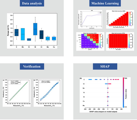
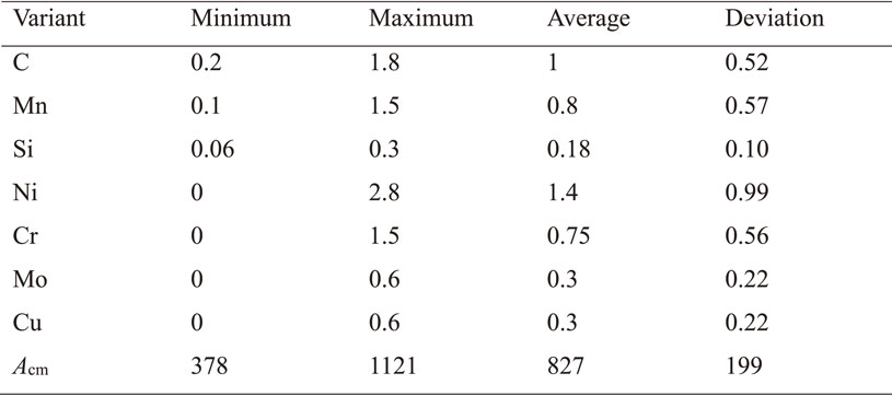
We collected 25,920 usable data points comprising the C, Mn, Si, Ni, Cr, Mo, Cu, and Acm temperatures. We then analyzed the dataset using a box plot. Figure 1 presents the box plot of the alloying elements. We could not confirm the outliers in the dataset. Therefore, we used all the datasets to train and test the machine learning models. The ranges of these datasets are listed in Table 1.

Box plots of the alloying elements.
We trained the ANN, SVR, and RFR models to predict the Acm temperature. We had to adjust the hyperparameters of the machine learning models to accurately predict the Acm temperature. The ANN model has hyperparameters such as the optimizer, number of neurons, number of layers, learning rate, and activation function of hidden layers.14,18) The SVR model has hyperparameters such as soft margins, type of kernel, kernel coefficient (γ), and regularization temperature parameter (C).19) The RFR model has hyperparameters such as the number of decision trees and the magnitude of the maximum depth of each decision tree.20,21) We adopted fivefold cross-validation to adjust the hyperparameters of the machine learning models. The hyperparameters of the ANN model were adjusted using a three-step process. We adopted adaptive moment estimation (Adam) as the optimizer for it. First, the learning rate was adjusted from 0.00001 to 0.1. Thereafter, an activation function was identified considering the sigmoid and rectified linear units (ReLu). Finally, the numbers of neurons in the first and second layers were determined using a grid search. We considered the number of neurons ranging from 1 to 50 for the first layer and from 0 to 50 for the second layer. The hyperparameters of the SVR model were determined using grid search by adjusting γ from 0.0000001 to 0.01 and C from 0.1 to 10,000. We applied a radial basis function as a kernel function. The hyperparameters of the RFR model were adjusted by changing the number of decision trees from 1 to 100 and the magnitude of the maximum depth of each tree from 1 to 100. To construct the SVR and RFR models, we divided the dataset into two parts: 75% as the training dataset and 25% as the test dataset. To construct the ANN model, we divided the dataset into three parts: 75% as the training dataset, 12.5% as the validation dataset, and 12.5% as the test dataset. We applied the determination coefficient (R2) to estimate the accuracy of the model. R2 can be expressed as follows:
| \begin{equation} R^{2} = \left(\frac{\displaystyle\sum [(x_{i} - \bar{x})(y_{i} - \bar{y})]}{\sqrt{\biggl[\displaystyle\sum (x_{i} - \bar{x})^{2}\biggr]\times \biggl[\displaystyle\sum (y_{i} - \bar{y})^{2}\biggr]}}\right)^{2} \end{equation} | (2) |
The results of hyperparameter adjustment are presented in Fig. 2. Figures 2(a) and (b) depict the adjustment of the hyperparameters of the ANN model. First, we determined the best learning rate for the ANN. The result is presented in Fig. 2(a). In this process, we set 50 neurons in the first and second layers and the ReLu of the activation functions of the first and second layers. A learning rate of 0.01 indicates the best performance as R2 = 0.999850 and 0.999847 for the training and test datasets, respectively. Thereafter, the activation function was adjusted by considering the sigmoid and ReLu functions. We set the other hyperparameters as 50 neurons in the first and second layers and a learning rate of 0.01. The result of setting the sigmoid function for the first and second layers is R2 = 0.999976 for the training dataset; the result of setting the ReLu function for the first and second layers is R2 = 0.999845 for the training dataset; the result of setting the ReLu function for the first layer and sigmoid function for the second layer is R2 = 0.999975 for the training dataset; and the result of setting the sigmoid function for the first layer and ReLu function for the second layer is R2 = 0.999972 for the training dataset. Therefore, we adopted the sigmoid function as the activation function for the first and second layers. Finally, the number of neurons in the hidden layers was determined. We illustrate the grid search results of the number of neurons in the hidden layers in Fig. 2(b). The results of the grid search demonstrate that R2 ≈ 1. Nevertheless, we selected the number of neurons that yielded the best value of R2 for the hidden layer. Therefore, we selected 32 neurons for the first layer and 31 neurons for the second layer. This model had R2 = 0.999997. Figure 2(c) illustrates the hyperparameters of the SVR model. In this result, C (10,000) and γ (0.01) lead to the best performance, that is, R2 = 0.998088. Figure 2(d) illustrates the hyperparameters of the RFR model. The adjustment of the RFR hyperparameters leads to R2 ≈ 1. Therefore, we could not confirm the best hyperparameters in Fig. 2(d). However, a maximum depth of 53 for each tree and 100 decision trees indicated the best performance, with R2 = 0.999976. Consequently, we set the learning rate to 0.01 and use the sigmoid function for the hidden layer and 32 and 31 neurons for the first and second layers, respectively, to predict Acm using the ANN model. We set C = 10,000 and γ = 0.01 to predict Acm using the SVR model. Finally, we set the maximum depth of each tree as 53 and use 100 decision trees to predict the value of Acm using the RFR model.

Results of hyperparameter optimization: (a) Line plot of the train and test R2 of ANN, (b) ANN, (c) SVR, and (d) RFR models.
Table 2 summarizes the performances of all the machine learning models, which were adjusted for hyperparameters. The ANN model demonstrated the best performance with R2 = 0.999997 for the training and test datasets. Thus, we chose the ANN model to analyze the mechanisms of the Acm prediction.
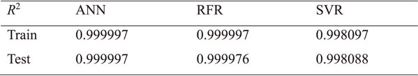
Figure 3(a) depicts the performance of the ANN model, which demonstrates close to perfect accuracy on the dataset. This model is illustrated to sufficiently predict the Acm temperature. Figure 3(b) illustrates the performance of eq. (1) for the dataset. Equation (1) yields R2 = 0.998054 and the ANN model yields R2 = 0.999997. This means that the ANN model predicts the Acm temperature more accurately, without a prediction error.

Comparison between the measured and predicted Acm temperatures: (a) Performance of the ANN model; (b) performance of eq. (1).
The SHAP method was applied to analyze the Acm temperature prediction mechanisms of the variables. Figure 4(a) illustrates the significance of each variable for the Acm temperature. The arithmetic mean of the absolute Shapley values for each variable was calculated to understand their average impact on the Acm temperature. C had the most significant impact on the Acm temperature, followed by Cr, Mn, Si, Ni, Cu, and Mo. This demonstrates the order of priority of their effect of the Acm temperature. Figure 4(b) illustrates the scatter plot of each variable to verify its effect on the Acm temperature. C, Cr, Mn, Si, and Mo appeared to increase the Acm temperature. Cu and Ni appeared to decrease the Acm temperature. However, we cannot exactly understand the effect of these variables on the Acm temperature. Therefore, we need to carefully analyze their effect on the Acm temperature.

Variable analysis of the ANN model using SHAP. (a) The average impact of each variable on the Acm temperature. (b) SHAP scatter plot of variables related to the Acm temperature.
We analyzed the detailed mechanisms of each variable using the SHAP dependence plot presented in Fig. 5. This illustrates the mean effect of variables on the Acm temperature. We adopted the base value of 853.80°C. Each point in the dependence plot represents the average variation from the base value. For instance, if the SHAP value is 0, the average Acm temperature is 853.80°C. If the SHAP value is 10, the average Acm temperature is 863.80°C. If the SHAP value is −10, the average Acm temperature is 843.80°C.

SHAP dependence plots for the variables.
Figure 5(a) illustrates the effect of C on the Acm temperature, which gradually increases with an increase in the C content. This is because, if C increases, it is saturated in the austenite phase. Therefore, the surplus C interacts with the Fe atoms to form cementite. Under approximately 0.8 wt% C, Cr increases the Acm temperature. At this C content, the primary ferrite and austenite phases transform into primary ferrite and pearlite phases. Therefore, Cr, which is well known as a ferrite stabilizer, exists in the primary ferrite phase with a high probability. It appears that Cr accelerates the release of C in the austenite phase. However, over approximately 0.8 wt% C, Cr decreases the Acm temperature. At this C content, the austenite phase transforms into the austenite and cementite phases. The cementite phase is generated at the austenite grain boundaries. However, Cr, which exists in the austenite phase, hinders the diffusion of C. Therefore, for this C content, Cr decreases the Acm temperature. Figure 5(b) depicts the effect of Cr on the Acm temperature. As Cr is a ferrite stabilizer, if the Cr content increases, the Acm temperature increases. Under approximately 0.8 wt% Cr, C increases the Acm temperature. However, beyond this value, C decreases the Acm temperature. Over 0.8 wt% Cr, it seems that an increase in the C content leads to the formation of M7C3 instead of the cementite phase.22) Therefore, C decreases the Acm temperature. Figures 5(c), (d), and (g) illustrate the Mn, Si, and Mo mechanisms, respectively. These alloying elements increase the Acm temperature. Figures 5(e) and (f) illustrate the Ni and Cu mechanisms, respectively. These alloying elements decrease the Acm temperature. Mn, Si, and Mo are known as carbide stabilizers and formers. Therefore, they seem to increase the Acm temperature. Cu and Ni are present in the ferrite phase and stabilize it. Thus, they seem to decrease the Acm temperature.2) These mechanisms help to understand the Acm temperature. Consequently, the Acm temperature can be controlled. The mechanisms can also be applied to heat treatment.
In this study, we propose machine learning models to predict the Acm temperature. We applied data analysis, hyperparameter adjustment, machine learning training, comparison of machine learning with the existing equation, and the SHAP method to understand the prediction mechanisms of the Acm temperature. Therefore, a dataset comprising alloying elements and the Acm temperature was collected and analyzed to detect outliers. No outliers were detected in the dataset. The hyperparameters for the ANN, SVR, and RFR models were determined; they demonstrated the best performances. The ANN model was chosen based on the value of R2. It was confirmed that the ANN model was more accurate than the empirical equation. Consequently, the significance and mechanisms of the variables used to predict the Acm temperature were understood. The C content had the most significant effect on the Acm temperature, followed by Cr, Mn, Si, Ni, Cu, and Mo. For a more detailed analysis, the SHAP dependence plots were adopted. In addition, the intimate mechanisms of the variables were discussed.
This work was supported by a Korea Institute for Advancement of Technology grant, funded by the Korea Government (MOTIE) (P0002019), as part of the Competency Development Program for Industry Specialists.