Abstract
Acoustic emission (AE) method enables real-time monitoring of damage initiation and progression. Recently, AE analysis using machine learning has become widely popular; however, the AE source location is often located manually to ensure reliability and accuracy. Therefore, it is desirable that the detection of AE source location is fully automated with a high accuracy. This study proposes a novel arrival time identification method for AE source location that can accurately and automatically locate AE sources. First, a wavelet transform is applied to an AE signal to extract the wavelet coefficient of a specific frequency. Subsequently, the Akaike information criterion is applied to the time transient of wavelet coefficient to identify the initial wave arrival time. The localized AE source accuracy is compared with conventional arrival time identification methods: visual initial wave arrival time identification, visual S0 mode arrival time identification at the time transient of the wavelet coefficients, automatic peak identification at the time transient of the wavelet coefficients, and automatic AIC wave arrival time identification. The proposed method reduces the number of events with incorrect initial arrival detections. Moreover, the correct detection rate increases by 1.5 times compared to a normal AIC. In addition, the proposed method is approximately 30 times faster than the conventional visual method and is an excellent AE wave arrival time identification in terms of both accuracy and speed of analysis. Lastly, we verify that the proposed method can be effectively applied to anisotropic materials.
1. Introduction
Acoustic emission method is a nondestructive testing technique to detect the initiation and propagation of damage in real-time. The source location is one of the methods for analyzing AE, which uses multiple sensors to identify the location of the AE source, depending on the difference in the arrival times of the signals detected by the sensors. Consequently, this helps analyze the AE signals, considering that detecting the AE source location clarifies the damage process. Furthermore, the AE sources can be accurately located by manually determining the initial wave arrival time of each AE waveform. However, considering that manually checking waveforms is challenging, an automatic analysis method is required in an environment that generates significant amounts of AE signals. Additionally, in recent years, AE analysis using machine learning has become popular; however, it requires full automation. Since then, several methods have been developed to determine the arrival time of AE signals automatically.
Several techniques for locating the AE source location, such as using the Akaike information criterion (AIC),1–3) wavelet transforms,4,5) mode or frequency wave speed differences,6–8) machine learning,9,10) etc.11–13) have been proposed. AIC is used in various fields to identify the initial arrival time of waveforms14–16) and the initial arrival time of AE signals.17) However, for small AE signal waveforms, the initial wave part is hidden in noise; therefore, the rise time cannot be measured correctly.18) The time-frequency information of AE is essential19–22) for both metals and composite materials.23) However, when the wavelet transform is used, the wavelet coefficient peak is often used as a reference; although, errors are likely to occur because of reflected waves for objects with complex shapes. Additionally, methods such as machine learning require a learning process and parameter settings when used in different situations.10)
Furthermore, few methods can be used with anisotropic materials, such as composites.24–30) Several methods for calculating the source location in anisotropic materials use frequency whose propagation velocity does not depend significantly on the angle of AE source and sensor location. However, the usable frequency is limited, considering the available frequency based on the situation.
This study proposes a novel wave arrival time identification method for AE source location with high accuracy that functions automatically under various conditions by using AIC and wavelet transform for thin plate members. The proposed method was first used to evaluate the calculated location accuracy by using an artificial AE source. Subsequently, the accuracy of the developed method was compared to those of conventional methods.
2. Experimental Method for AE Source Location Accuracy Using an Artificial AE Source and the Developed Method
2.1 Experimental setup
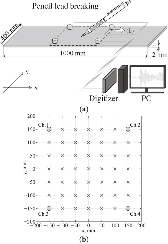
Figure 1 shows the experimental setup. Four AE sensors were placed in the center of a 2 mm thick aluminum plate (A1100P, L × W = 1000 mm × 400 mm) in a 300 mm × 300 mm area. Artificial sources were excited at 50 mm intervals between the sensors. Hsu–Nielsen source, which is most commonly used for Artificial AE, was used because it emits a wide frequency bandwidth. AE signal measurement resolution was 8192 points at 50 ns intervals. Artificial AE signals were excited at each source position, and two AE signals were randomly selected for verification. Three types of resonant AE sensors (PAC: PICO, R15α, and R50α) were used, as shown in Table 1. Herein, we evaluated the accuracy of different wave arrival time identification methods and the differences in the accuracy of the sensors used.
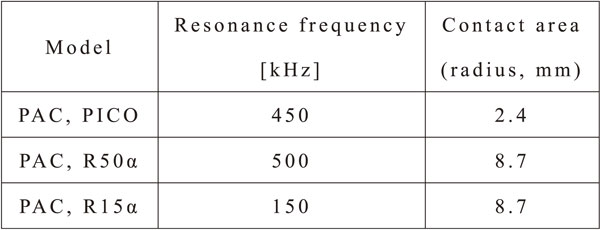
Table 1 Resonant frequency and size of sensors.
Figure 2 shows the algorithm of the proposed wave arrival time identification method and source location flowchart. As an example for describing the method below, we used the pencil lead breaking AE input at (x, y) = (−100.0, 50.0) with the PICO sensor location at channel 1. First, the measured AE waveform (Fig. 2(Step. 0)) was wavelet transformed to create a wavelet contour map (Fig. 2(Step. 1)). The mother wavelet of the wavelet transforms used in this study was Gabor function. Subsequently, the time transient of the wavelet coefficients at a specific frequency was extracted (Fig. 2(Step. 2)). We extracted the resonance frequency of the PICO sensor, i.e., 450 kHz. Lastly, AIC was applied to automatically read the arrival time of the initial wave for the time transient of the wavelet coefficient (Fig. 2(Step. 3)). The developed method is useful for thin plates with strong Lamb waves because an arrived initial wave at a specific frequency must be known.

The evaluation of AIC was defined by the following relation, which applies the maximum likelihood method to adjust the parameters for maximizing the likelihood of the observed data:31)
| \begin{align}
\text{AIC}& = (-2) \log (\text{maximum likelihood})\\
&\quad + 2 (\text{number of adjusted parameters})
\end{align}
| (1) |
Based on this equation, the formula was refined to identify discontinuities in the data, expressed as given below. AICk at the point i = k with amplitude value Xi (i = 1, 2, …, N) was calculated for a single AE waveform recorded with N number of samples, given as:
32)
| \begin{align}
\text{AIC}_{\text{k}} &= \text{k}\cdot \log\{\mathop{\text{var}}\nolimits(\text{X}[1,\text{k}])\} \\
&\quad+ (\text{N} - \text{k}) \cdot \log\{\mathop{\text{var}}\nolimits(\text{X}[\text{k},\text{N}])\}
\end{align}
| (2) |
where var(X[1, k]) and var(X[k, N]) are the variance of amplitude value from X
1 to X
k and X
k to X
N, respectively. Finally, k of AIC
k minimum value indicates the arrival time of the AE signal.
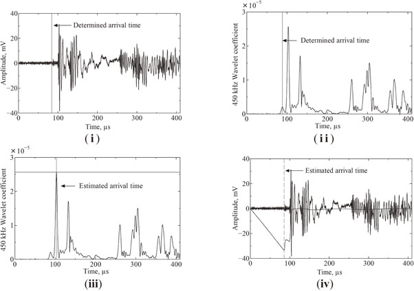
As shown in Fig. 2(Step. 3), the arrival time of the initial wave was calculated as 81.80 µs. Subsequently, the arrival times for all sensors were calculated. Finally, the calculated arrival times were used to calculate the AE source location using the virtual sound source scanning method. This method defines the location area and calculation resolution. The difference between the theoretical arrival time and the actual arrival time at each point within the virtually defined area is compared as shown in Fig. 2(Step. 4), and the location with the smallest difference is designated as the AE source (Fig. 2(Step. 5)). Calculations were performed with a resolution of 0.1 mm within the range of the sensor. Figure 3 shows an existing method that compares the accuracy of the developed method with that of the previously used method. The following four methods were used.
-
(i)
Manual identification of the arrival time of S0 mode first wave of the detected wave.33)
-
(ii)
A method to manually identify the arrival time of the S0 mode initial wave of the Lamb wave of the time transient of the wavelet coefficient.4)
-
(iii)
A method to automatically identify the peak time using the time transient of the wavelet coefficient.4)
-
(iv)
A method to automatically identify the initial arrival time of a waveform using AIC for the detected wave.32)
Lamb waves mainly propagate in thin plates.34) Figure 4 shows the Lamb wave theoretical group velocity dispersion curve for a 2-mm thick aluminum plate. This velocity was used for theoretically calculating the wave arrival time. When waveforms were used (method (i) and (iv)), sheet velocities (5355 m/s) were used; when wavelet coefficients were used (method (ii), (iii), and the proposed method), group velocities at wavelet-transformed frequencies were used.
3. Result and Discussions
3.1 Evaluation of AE source location accuracy with conventional methods
Figure 5 compares the results of the proposed method and conventional methods for AE source location. The left side of the figure demonstrates the results by using the PICO sensor, whereas the right side of the figure shows the error distribution of the results. On comparing the results, it was found that the automatic reading method (iii, iv) resulted in a larger error than the method that visually read the initial wave (i, ii), owing to the errors in reading the initial arrival time. Conversely, the proposed method demonstrated a lower error rate despite the automatic initial reading, confirming its superiority as a wave arrival time identification.

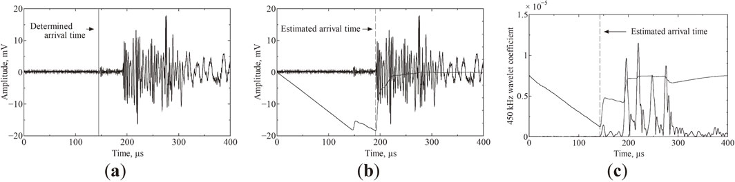
Figure 6 shows one of the results input at (−100, 100). Figure 7 shows the identified time of ch. 4, considering ch. 4 has the longest distance in the four channels at this point. While the manual method (Fig. 7(a)) presumably identified the initial arrival time correctly, AIC (Fig. 7(b)) identified the arrival time of the Lamb wave A0 mode on behalf of the S0 mode. Considering this arrival time identification, the located source location by AIC was far from the target on the opposite side of the ch. 4 sensor, considering AIC identified the Lamb wave A0 mode as S0 mode, which delays the arrival time. Conversely, the manual identification was accurate. The actual located source location shifted on the opposite side of the ch. 4, similar to the AIC result. This verifies the efficiency of the proposed method in situations having a long-distance between the source and sensor locations.

Figure 8 compares the analysis time for each method. The method of reading manually depends on the skill of the engineer. In this case, the data was obtained by an engineer with approximately two years of AE analysis experience. The automatic reading method ((iii), (iv), proposed method) is approximately 30 times faster than the visual method ((i), (ii)) and does not depend on the skill of the operator. The improved speed of the proposed method is essential for data analyses. Therefore, the developed method is an excellent AE wave arrival time identification in terms of accuracy and analysis speed.
3.2 Relationship between sensor characteristics and source location accuracy
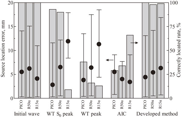
Figure 9 shows the difference in the source location accuracy between the AIC-based method and the proposed method using three types of sensors (PICO, R50α, and R15α). The AIC-based method showed that the difference in the accuracy of the detection sensitivity of the three sensors (PICO, R50α, and R15α) was significantly large, owing to the sensor’s contact area size. Because the piezoelectric element inside the AE sensor converts vibration into voltage, the amplitude of the signal detected by the sensor is the integral of the vibration-to-voltage conversion efficiency per unit area of the piezoelectric element over the installed area of the sensor. Moreover, a pencil lead breaking AE tends to compose low-frequency, and the resonance frequency of the R15α sensor is 150 kHz, which is lower than that of the PICO and R50α sensors. In the case of initial arrival wave identification using AIC, the used velocity in the virtual sound source scanning method is the fastest propagation velocity in the lamb wave for all frequencies. The thin plate S0 mode propagation velocity tends to decrease at high frequencies. Therefore, a sensor with a high resonant frequency would be less sensitive to fast low-frequency waves and result in a source location error. Thus, R15α sensor exhibits a small error. Additionally, the distribution of error and frequency was divided into two parts: error of less than 10 mm and error of more than 10 mm. We checked some of this data. For all four channels with errors less than 10 mm, AIC correctly identified the initial arrival time. However, AIC did not correctly identify the initial arrival time in one or more channels having larger errors.

Figure 10 shows the source location error histogram. All three sensors had a single normal distribution, unlike the previous result. There were only a few sensors with large errors, which indicated that the AIC incorrectly read the initial arrival time, as well as AIC applied for the waveform.
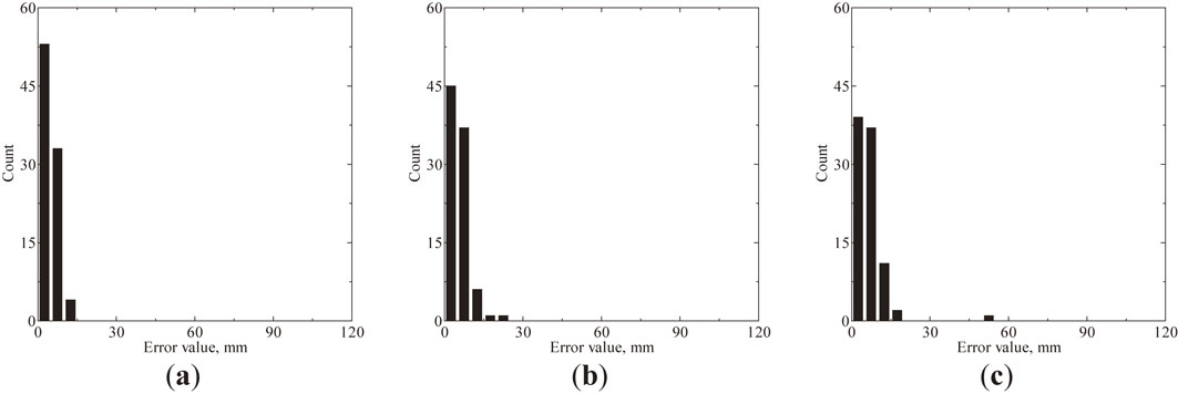
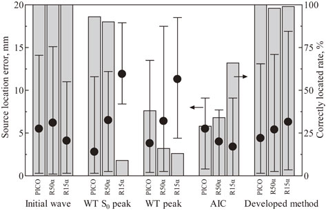
Figure 11 shows the average source location accuracy for each sensor and the percentage of AE signals correctly identified for all the methods. The percentage of “correctly identified” is a targeting error of 19 mm or more equivalent to the largest sensor diameter. Comparing the percentage of correctly identified AE signals, the visual initial wave detection and the developed method could correctly locate the position with an accuracy of more than 90%. This source location error is approximately equal to manual initial detection and the developed method. In contrast, the other methods failed in more than 50% of the cases. The developed method’s source location accuracy was acceptable. Furthermore, it was confirmed that the developed method is approximately as accurate as the method that detects the initial arrival time visually without relying on a sensor.
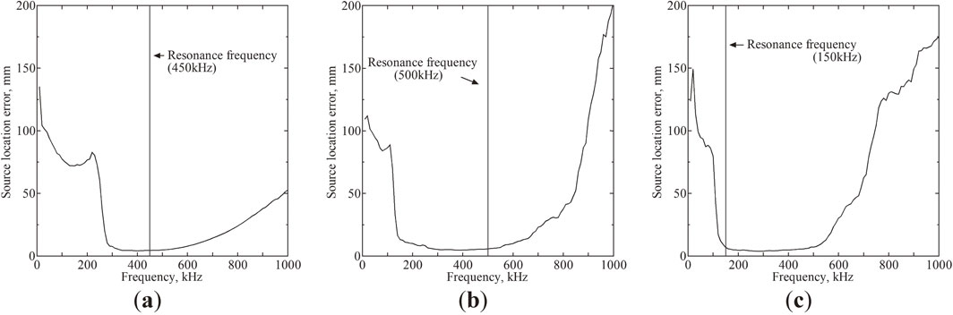
Next, we evaluated the frequency at which the wavelet coefficients were extracted from the AE signals detected by the three sensors, and the source location accuracy. The relationship between frequency and location error is shown in Fig. 12. There is a correlation between the sensor’s resonant frequency bandwidth and the signal-to-noise ratio (S/N), but the magnitude of the S/N does not correspond to the error size. The location error for the PICO and R50α sensors was low near the resonance frequency. Conversely, the accuracy of the R15α sensor decreased significantly at frequencies lower than the resonance frequency, which was common with the results of the three sensors. This can be attributed to the fact that the slope of the initial wave of the wavelet coefficients in the wavelet transform becomes more gradual as the frequency decreases, making it difficult to identify discontinuities due to AIC. Therefore, when using this new method, AE sensors with resonance frequencies above 200 kHz must be used for accurate targeting or selecting the second resonance frequency above that frequency.
In this study, although we did not compare the accuracy of this method with that of machine learning and deep learning methods, we believe this method is very versatile, considering it is a simple algorithm.
4. Application to an Anisotropic Material
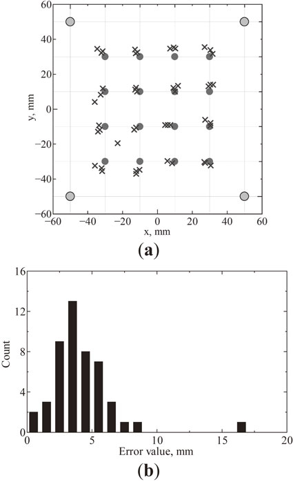
The purpose of the current study was to perform highly accurate and automatic source location calculations of anisotropic materials such as CFRP. Therefore, experiments were conducted using an artificial AE source with plain-woven CFRP to confirm the accuracy of the developed method. The experimental setup is shown in Fig. 13. A pencil lead breaking as an artificial AE source was input at intervals of 20 mm in both the X- and Y-directions at the center of a 2 mm thick plain-woven CFRP plate (L × W = 200 mm × 200 mm) in a 100 mm × 100 mm area. Artificial AE signals were excited five times at each source position and three AE signals were selected randomly for verification. The sensors used were PAC, PICO: resonance frequency 450 kHz. A sine approximation based on the measured propagation sheet velocity, 5897 m/s for 0° and 90° and 4546 m/s for 45°, was employed when using the virtual sound source scanning method.
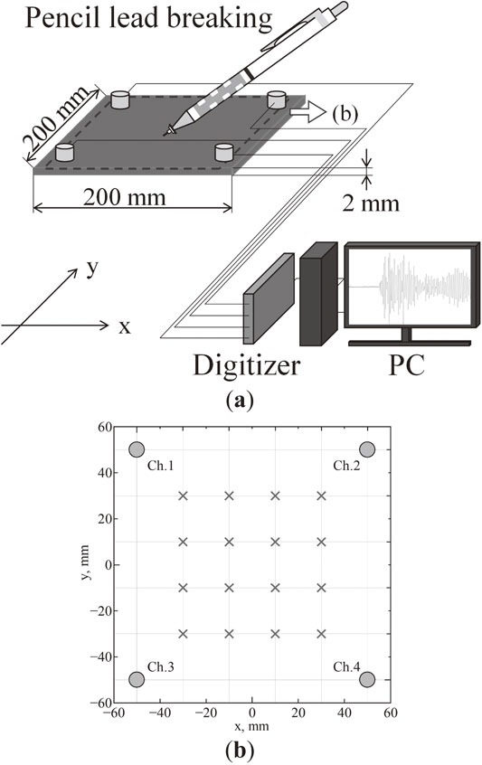
Figure 14 shows the source location result and the error distribution of the source location. In these results, a sine approximation based on the measured propagation velocity of 450 kHz; 5838 m/s for 0° and 90°, 4499 m/s for 45°, was used. One of the AE signals deviated by 16.0 mm, which is significant devitaion, but the other calculated results were less than 10 mm, and the average error was 4.1 mm, within the diameter of the sensor. Thus, the source location accuracy from the proposed method is sufficient. Moreover, its effectiveness for anisotropic materials is confirmed.
5. Conclusion
In this study, we proposed a novel method for AE source location with high accuracy that functions automatically by using AIC and wavelet transform. We compared the accuracy of the proposed method with various conventional methods using artificial AE of pencil lead breakage. Although the proposed method was not highly accurate, it was effective in fully automated localizing of the detected AE signals while considering the accuracy and AE location correctly. Furthermore, we confirmed that the accuracy of AE location detection changes depending on the frequency and that the resonance frequency of the sensor can be used to achieve high accuracy at a frequency of 200 kHz or higher. Lastly, we verified that the proposed method can be effectively applied to anisotropic materials.
REFERENCES
- 1) M.R. Pearson, M. Eaton, C. Featherston, R. Pullin and K. Holford: Struct. Health Monit. 16 (2017) 382–399. doi:10.1177/1475921716672206
- 2) J. Hensman, R. Mills, S.G. Pierce, K. Worden and M. Eaton: Mech. Syst. Signal Process. 24 (2010) 211–223. doi:10.1016/j.ymssp.2009.05.018
- 3) P. Sedlak, Y. Hirose, S.A. Khan, M. Enoki and J. Sikula: Ultrasonics 49 (2009) 254–262. doi:10.1016/j.ultras.2008.09.005
- 4) H. Jeong and Y.S. Jang: IEEE Trans. Ultrason. Ferroelectr. Freq. Control 47 (2000) 612–619. doi:10.1109/58.842048
- 5) J. Jiao, C. He, B. Wu, R. Fei and X. Wang: Front. Mech. Eng. China 1 (2006) 341–345. doi:10.1007/s11465-006-0006-4
- 6) A. Mostafapour, S. Davoodi and M. Ghareaghaji: Ultrasonics 54 (2014) 2055–2062. doi:10.1016/j.ultras.2014.06.022
- 7) M.G. Baxter, R. Pullin, K.M. Holford and S.L. Evans: Mech. Syst. Signal Process. 21 (2007) 1512–1520. doi:10.1016/j.ymssp.2006.05.003
- 8) J. Jiao, C. He, B. Wu, R. Fei and X. Wang: Int. J. Press. Vessels Piping 81 (2004) 427–431. doi:10.1016/j.ijpvp.2004.03.009
- 9) L. Cheng, H. Xin, R.M. Groves and M. Veljkovic: Constr. Build. Mater. 273 (2021) 1–17. doi:10.1016/j.conbuildmat.2020.121706
- 10) M.A. Pillai, A. Ghosh, J. Joy, S. Kamal, C.C. Satheesh, A.A. Balakrishnan and M.H. Supriya: 2019 International Symposium on Ocean Technology (SYMPOL) (IEEE, Ernakulam, India, 2019) pp. 191–199.
- 11) B.A. Zárate, A. Pollock, S. Momeni and O. Ley: Smart Mater. Struct. 24 (2015) 015017. doi:10.1088/0964-1726/24/1/015017
- 12) A. Ebrahimkhanlou and S. Salamone: Ultrasonics 78 (2017) 134–145. doi:10.1016/j.ultras.2017.03.006
- 13) A. Ebrahimkhanlou and S. Salamone: Aerospace 5 (2018) 50. doi:10.3390/aerospace5020050
- 14) N. Maeda: Zisin J. Seismol. Soc. Jpn. 2nd Ser. 38 (1985) 365–379. doi:10.4294/zisin1948.38.3_365
- 15) R. Sleeman and T.V. Eck: Phys. Earth Planet. Inter. 113 (1999) 265–275. doi:10.1016/S0031-9201(99)00007-2
- 16) H. Zhang, C. Thurber and C. Rowe: Bull. Seismol. Soc. Am. 93 (2003) 1904–1912. doi:10.1785/0120020241
- 17) J.H. Kurz, C.U. Grosse and H.W. Reinhardt: Ultrasonics 43 (2005) 538–546. doi:10.1016/j.ultras.2004.12.005
- 18) D.G. Aggelis and T.E. Matikas: Comput. Struc. 98–99 (2012) 17–22. doi:10.1016/j.compstruc.2012.01.014
- 19) M. Niethammer, L.J. Jacobs, J. Qu and J. Jarzynski: J. Acoust. Soc. Am. 107 (2000) L19–L24. doi:10.1121/1.428894
- 20) H. Suzuki, T. Kinjo, Y. Hayashi, M. Takemoto and K. Ono: J. Acoust. Emiss. 14 (1996) 69–84.
- 21) Y. Ding, R.L. Reuben and J.A. Steel: NDT E Int. 37 (2004) 279–290. doi:10.1016/j.ndteint.2003.10.006
- 22) L. Ambrozinski, T. Stepinski, P. Packo and T. Uhl: Mech. Syst. Signal Process. 27 (2012) 337–349. doi:10.1016/j.ymssp.2011.09.019
- 23) H. Jeong: NDT E Int. 34 (2001) 185–190. doi:10.1016/S0963-8695(00)00056-6
- 24) Y. Mizutani, T. Miki, A. Todoroki and Y. Suzuki: 32nd European Conference on Acoustic Emission Testing (32nd EWGAE) (NDT, Prague, Czech Republic, n.d.) pp. 333–341.
- 25) M. Koabaz, T. Hajzargarbashi, T. Kundu and M. Deschamps: Struct. Health Monit. 11 (2012) 315–323. doi:10.1177/1475921711419991
- 26) T. Kundu, H. Nakatani and N. Takeda: Ultrasonics 52 (2012) 740–746. doi:10.1016/j.ultras.2012.01.017
- 27) M.R. Jones, T.J. Rogers, K. Worden and E.J. Cross: Mech. Syst. Signal Process. 163 (2022) 108143. doi:10.1016/j.ymssp.2021.108143
- 28) N. Toyama, J.H. Koo, R. Oishi, M. Enoki and T. Kishi: J. Mater. Sci. Lett. 20 (2001) 1823–1825. doi:10.1023/A:1012507821711
- 29) H. Yamada, Y. Mizutani, H. Nishino, M. Takemoto and K. Ono: J. Acoust. Emiss. 18 (2000) 51–60.
- 30) H. Jeong and Y.S. Jang: Compos. Struct. 49 (2000) 443–450. doi:10.1016/S0263-8223(00)00079-9
- 31) H. Akaike: in Selected Papers of Hirotugu Akaike, (Springer, New York, NY, 1998) pp. 387–410.
- 32) K. Ohno, S. Shimozono, Y. Sawada and M. Ohtsu: J. Jpn. Soc. Non-Destr. Insp. 57 (2008) 531–536. doi:10.11396/jjsndi.57.531
- 33) T. J. Society for Non-Destructive Inspect: Practical Acoustic Emission Testing, (Springer Japan, Tokyo, 2016).
- 34) M.N. Salim, T. Hayashi, M. Murase, T. Ito and S. Kamiya: Mater. Trans. 53 (2012) 610–616. doi:10.2320/matertrans.I-M2012801