Abstract
The homogenization method is effective for analyzing macroscopic mechanical properties from the substructure of a material. In perforated sheet metal, macroscopic mechanical properties depend on the pattern of hole arrangement. In this study, the macro–plastic properties of perforated sheets with 60° standard staggered and 90° square arrangements are modeled. Biaxial stress is applied to the unit cells given the periodic boundary condition, and the contours of equal plastic work are obtained. The yield surfaces of the perforated sheets on the tension–compression combined stress state are strongly affected by the hole arrangement. To model the yield surface, a yield function for the rotational symmetry peculiar to the perforated sheet is proposed. The yield surfaces are modeled using the CPB2006 yield function that takes into consideration tension–compression asymmetry. Also, a surface–interpolated differential hardening model is applied to model the changes of yield surfaces. The analysis results obtained using the modeled yield surfaces are compared with the experimental ones obtained on the uniaxial tensile and deep drawing tests. The results of both tests show good agreement.
This Paper was Originally Published in Japanese in J. JSTP 62 (2021) 118–125.
1. Introduction
The homogenization method is a scheme for analyzing the macroscopic mechanical properties from the microstructure (substructure) of a material.1,2) Using this method as a numerical material test enables the prediction of macroscopic properties from the morphology of the substructure and the design of the substructure to achieve the desired properties. To date, many studies have been conducted to obtain macroscopic properties from the arrangement and orientation of carbon fiber-reinforced plastics and texture information of polycrystalline metals.3,4) Many studies using homogenization method analysis deal with microscopic-level substructures; however, the examination of the accuracy of the analysis is focused on macro level validation. Meanwhile, in perforated sheet metal, in which holes are regularly arranged, the substructure is visible, so the validation of analysis accuracy at both the macro and substructure levels is possible.5–8)
In perforated sheet metal, the macro properties should change depending on the pattern of the hole arrangement.9) Therefore, these sheets are suitable as practical examples for modeling anisotropic plastic properties using homogenization method.10) Furthermore, the unique plastic anisotropies expressed in the properties of such artificially created sheet materials differ significantly from those of plain sheet metals. Therefore, the attempt to model a macro constitutive equation of perforated sheet metal is interesting as a touchstone for evaluating the expressibility of existing yield functions.
In this study, we used two types of perforated sheet metal with the same ratio of open area and different hole arrangements and obtained contours of equal plastic work by homogenization analysis. We propose a mathematical model that expresses the macro yield surface. In addition, the models were validated by comparing the analysis results obtained using the proposed macro constitutive equation and the experimental results of uniaxial tensile and cylindrical deep drawing tests.
2. Test Material and Analysis Method
2.1 Test material
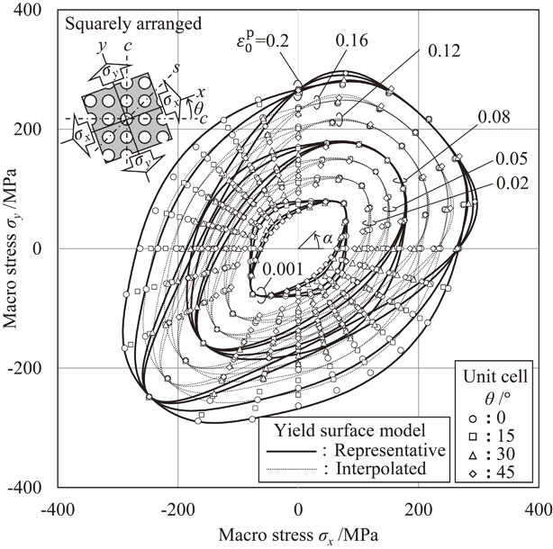
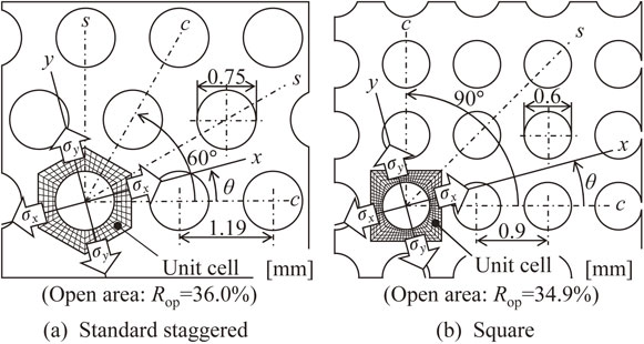
Figure 1 shows the hole arrangement and dimensions of the two types of perforated sheet metal used in this study. We used perforated sheet metal with a 60° staggered arrangement and 90° square arrangement. The in-plane orientation is described as the c (closed) direction in which the holes are placed closest and the s (sparse) direction in the middle of the two c directions. The ratio of the open area Rop was 36.0% for the staggered perforated sheet metal and 34.9% for the square perforated sheet metal. To clarify the effect of hole arrangement, we selected perforated sheet metals with similar open area ratios.
The base material of the perforated sheet metal was SUS304 cold-rolled stainless steel with a nominal thickness of 0.3 mm. Annealing heat treatment was carried out at 1080°C to reduce the anisotropy of the base material. Table 1 lists the mechanical properties of the base material. The analysis assumes a plane stress state, the von Mises isotropic yield condition and isotropic hardening to simplify the plastic properties of the base material. Subscript b is added to the symbols representing the stress and strain of the base material.

Table 1 Mechanical properties of base material.
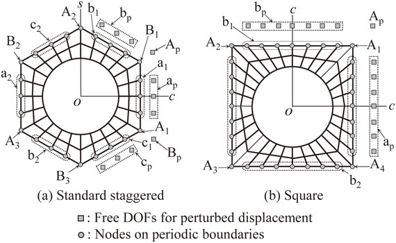
In this study, the computational homogenization method was used for the analysis of macro properties. The unit cell shapes used in the analysis were a regular hexagon in a staggered arrangement and a square in a square arrangement, and periodic boundary conditions were applied to all edges and vertices. Figure 2 shows a schematic illustration of the unit cells and their periodic boundary conditions. The unit cells were arranged periodically without gaps. Therefore, even if the outer edge is distorted owing to deformation, there should be no gaps or overlaps at the boundary. To represent the boundary distortion, the perturbation displacement increment {ΔuMp} is added as a common distortion to the nodes on equivalent edges and vertices on the circumference of the unit cells.
Denoting the macro true strain increment for the unit cell as {Δε}, the nodal displacement increment {ΔuMi} on the periodic boundary are represented by the following equation.
| \begin{equation}
\begin{Bmatrix}
\Delta u_{x}^{Mi}\\
\Delta u_{y}^{Mi}
\end{Bmatrix}
=
\begin{bmatrix}
x^{Mi} & 0 & \dfrac{y^{Mi}}{2}\\
0 & y^{Mi} & \dfrac{x^{Mi}}{2}
\end{bmatrix}
\begin{Bmatrix}
\Delta \varepsilon_{x}\\
\Delta \varepsilon_{y}\\
\Delta \gamma_{xy}
\end{Bmatrix}
+
\begin{Bmatrix}
\Delta u_{x}^{M\text{p}}\\
\Delta u_{y}^{M\text{p}}
\end{Bmatrix}
\end{equation}
| (1) |
Here, {xMi, yMi} indicates the current nodal coordinates on the outer circumference of the unit cell. The node group symbol Mi for the staggered perforated sheet is as follows.
| \begin{equation}
M = \text{A, B, a, b, c}\quad i =
\left\{
\begin{array}{c}
1,2,3\ (M = \text{A, B: Corner})\\
1,2\ (M = \text{a, b, c: Edge})
\end{array}
\right.
\end{equation}
| (2) |
For the squarely arranged perforated sheet, Mi is as follows.
| \begin{equation}
M = \text{A, a, b}\quad i =
\left\{
\begin{array}{c}
1,2,3,4\ (M = \text{A: Corner})\\
1,2\ (M = \text{a, b: Edge})
\end{array}
\right.
\end{equation}
| (3) |
The above-mentioned periodic boundary conditions were incorporated into the finite element analysis. The degrees of freedom of the perturbation displacement increment {ΔuMp} and the macro true strain increment {Δε} are set as the degrees of freedom of independent nodes that do not belong to the finite element model of the unit cell. The macro true stress {σ} loaded on the unit cell is applied as an external force to the degree of freedom of the macro true strain increment {Δε}.11) In this analysis, the macro true strain increment {Δε} and the micro perturbation displacement increment {ΔuMp} are solved by coupling with unit cell model.
The general-purpose nonlinear finite element analysis code Marc was used for the analysis. The coupling equation for the degrees of freedom shown in eq. (1) is incorporated into the user subroutine.12) Equivalent constraints can be set using a multipoint constraint function in other general-purpose analysis codes.
2.3 Calculation of equal plastic work contour
In this study, the postulate of equivalence of plastic work13) was assumed, and the contour of the equal plastic work was considered identical to the yield surface.14,15) As shown in Fig. 1, the true stress is applied to the unit cell as the principal stress in the coordinate system xy tilted by θ from the principal axis of anisotropy (c direction) of the perforated sheet metal. The angle θ between the axis of anisotropy and the axis of principal stress was varied in four steps from the c direction to the s direction for each perforated sheet metal. The ratio of biaxial stress is represented by α = tan−1(σy/σx) as the loading direction, and α is varied in 15° increments to analyze the all directions of the stress space.
The macro yield locus (contour of equal plastic work) was calculated as follows: First, the macro elastic matrix [De] of the perforated sheet metal is obtained from the elastic behavior before the initial yield. The increment of plastic work after yielding ΔWp is calculated by the following equation.
| \begin{equation}
\Delta W^{\text{p}} = \{\sigma\}^{\text{T}}\{\Delta\varepsilon^{\text{p}}\} = \{\sigma\}^{\text{T}}\{\{\Delta\varepsilon\} - [D^{\text{e}}]^{-1}\{\Delta\sigma\}\}
\end{equation}
| (4) |
Macro stress point {σ} are connected where the plastic work Wp, which is the accumulation of ΔWp is equal, and this locus is the contour of equal plastic work. The level of equal plastic work is expressed by the tensile plastic strain based on the plastic work in the c direction uniaxial tension; this is referred as the reference plastic strain $\varepsilon_{0}^{\text{p}}$.16)
3. Analysis Results and Discussion of Contour of Equal Plastic Work
3.1 Analysis results
Figure 3 shows the plots of the equal plastic work points calculated for the staggered and squarely arranged perforated sheet metals. The angle θ between the axes of anisotropy and principal stress is varied in four steps and distinguished by the symbols (○□△◇). The lines in the figure are described in section 4.5.
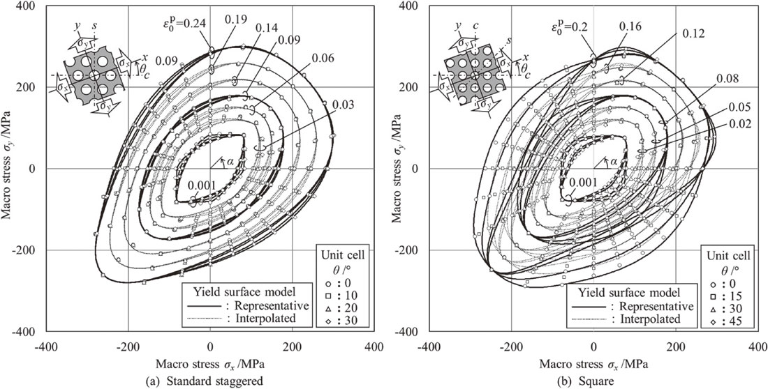
The yield locus of the staggered perforated sheet metal shown in Fig. 3(a) shows an acutely bulging shape in the equibiaxial direction at the initial yield when $\varepsilon_{0}^{\text{p}} = 0.001$. The plots dispersed under uniaxial tension and compression indicate a high in-plane anisotropy in the uniaxial stress state. As the plastic deformation progressed, the variance of the plot points decreased, and at $\varepsilon_{0}^{\text{p}} = 0.09$, the yield locus became almost in-plane isotropic. However, when the plastic deformation progresses further, an in-plane anisotropy different from the initial yield locus appears in the second and fourth quadrants (combined stress states of tension and compression). In addition, the yield locus at $\varepsilon_{0}^{\text{p}} = 0.24$ shows an egg shape tapered to equibiaxial compression, and there is a remarkable tensile/compressive asymmetry that was not observed in the initial yield locus.
The yield locus of the squarely arranged perforated sheet metal shown in Fig. 3(b) exhibits high in-plane anisotropy in the second and fourth quadrants at the initial yield ($\varepsilon_{0}^{\text{p}} = 0.001$). Unlike the staggered arrangement, the high in-plane anisotropy in this stress state remains even as plastic deformation progresses. In addition, with the progress of plastic deformation, in-plane anisotropy that was not observed on the initial yield locus appears even at α = 15° and 75° in the first quadrant. The yield locus of the squarely arranged sheet shows the differential hardening in which the stress ratio of high anisotropy changes with the progress of plastic deformation.
As described above, the yield surface shows clear differential hardening for both hole arrangements. In addition, when plastic deformation increases, the asymmetry of tension and compression becomes apparent.
3.2 Discussion
Using the homogenization method, the reason for the appearance of macro properties can be explained in detail from the deformation of the unit cell. In this section, the difference in the shape of the yield locus owing to the arrangement of holes is discussed based on the deformation of the substructure. The yield loci of the two types of perforated sheet metal show a large difference in the second and fourth quadrants, in which tension and compression are combined. Figure 4 shows the deformation state of the unit cell on α = −45° (pure shear stress in the fourth quadrant) at $\varepsilon_{0}^{\text{p}} = 0.1$, in the case that the axis of principal stress coincides with the c and s directions. The color of the deformed finite element mesh shown in the upper row indicates the distribution of the equivalent plastic strain $\bar{\varepsilon }_{\text{b}}^{\text{p}}$ of the base material. The lower row shows schematic illustrations of the transmission path of tensile and compressive loads.
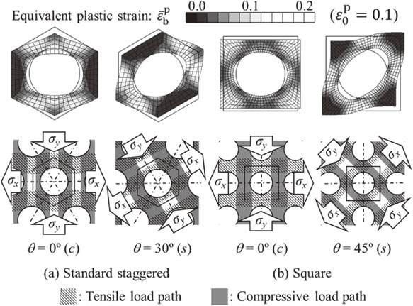
In the staggered arrangement shown in Fig. 4(a), the load transmission paths of tension and compression are switched at θ = 0° and θ = 30°. However, the region where these load paths overlap is the common position of the c-direction ligament (skeleton) where the inter-hole distance is the smallest. The equivalent plastic strain ($\bar{\varepsilon }_{\text{b}}^{\text{p}}$) distribution of the base material shown in the upper row shows that large plastic deformation concentrates in the same ligaments. Therefore, the in-plane anisotropy is small in the second and fourth quadrants. On the other hand, in the square arrangement shown in Fig. 4(b), on θ = 0°, the load transmission paths of tension and compression overlap in the s-direction ligaments with the long inter-hole distance. However, on θ = 45°, the transmission paths overlap in the c-direction ligaments with the smallest inter-hole distance. Therefore, in the square arrangement, the yield loci expand or contract in the second and fourth quadrants depending on the width of the ligament in which the combined load of tension and compression is applied.
4. Modeling of the Macro Yield Surface
As previously mentioned, the macro plastic properties of perforated sheet metal exhibit differential hardening and tensile/compressive asymmetry. Additionally, because of the periodicity of the hole arrangement, the same macro properties should appear for the coordinate rotations every 60° in the staggered arrangement and every 90° in the square arrangement. In this section, we describe a method to incorporate these features into the yield function.
4.1 Asymmetry of tension and compression
Although a simple von Mises yield condition is assumed for the base material, tensile/compressive asymmetry appears on the macro yield surface because the substructure (hole shape and inter-hole distance) changes with deformation in the perforated sheet metal. This asymmetry is called the strength-differential (SD) effect.
Several yield functions have been proposed to express the SD effect.17,18) In perforated sheet metal, the initial yield surface has the feature of an acutely bulging shape in the equibiaxial direction. Therefore, the use of a higher-order yield function is appropriate. In this study, the yield function proposed by Cazacu et al. (hereinafter, CPB2006) was used.17)
4.2 Mathematical expression of differential hardening
In a perforated sheet metal, the shape of the yield surface changes with the plastic deformation. Therefore, a differential hardening model was used for the hardening rule. Here, the equivalent plastic strain ($\bar{\varepsilon }^{\text{p}}$), which is the simplest scalar value representing the amount of plastic deformation, was used as a parameter to represent the progress of differential hardening. The general formula for the yield condition of differential hardening is
| \begin{equation}
\bar{\sigma}(\sigma_{ij},\bar{\varepsilon}^{\text{p}}) - H(\bar{\varepsilon}^{\text{p}}) = 0.
\end{equation}
| (5) |
Here, $H(\bar{\varepsilon }^{\text{p}})$ is the true stress-true plastic strain curve (deformation resistance curve) of the uniaxial tensile test in the reference direction (c direction). Note that $\bar{\varepsilon }^{\text{p}}$ in this study is synonymous with the reference plastic strain $\bar{\varepsilon }^{\text{p}}_{0}$ when finding the equal plastic work contour.
Various expressions have been proposed for the differential hardening model.19) In this study, we used a surface-interpolated model that is easy to implement in finite element analysis.20,21) In this model, the characteristic surfaces of the differentially hardened yield surface were used as the representative surfaces, and the arbitrary yield surface between them was interpolated using a simple function. The equivalent plastic strains on the representative yield surface are $\bar{\varepsilon }_{\text{A}}^{\text{p}}$ and $\bar{\varepsilon }_{\text{B}}^{\text{p}}$ ($\bar{\varepsilon }_{\text{A}}^{\text{p}} < \bar{\varepsilon }_{\text{B}}^{\text{p}}$), and each representative yield surface is defined by the following equation:
| \begin{equation}
\left\{
\begin{array}{l}
\bar{\sigma}_{\text{A}}(\sigma_{ij}) - H(\bar{\varepsilon}_{\text{A}}^{\text{p}}) = 0\\
\bar{\sigma}_{\text{B}}(\sigma_{ij}) - H(\bar{\varepsilon}_{\text{B}}^{\text{p}}) = 0
\end{array}
\right.
\end{equation}
| (6) |
Here, $\bar{\sigma }_{\text{A}}(\sigma_{ij})$ and $\bar{\sigma }_{\text{B}}(\sigma_{ij})$ are yield functions for the representative surfaces. When $\bar{\varepsilon }^{\text{p}}$ satisfies $\bar{\varepsilon }_{\text{A}}^{\text{p}} \leq \bar{\varepsilon }^{\text{p}} \leq \bar{\varepsilon }_{\text{B}}^{\text{p}}$, the yield surface at $\bar{\varepsilon }^{\text{p}}$ is expressed by the following equation.
| \begin{align}
&\mu(\bar{\varepsilon}^{\text{p}})(\bar{\sigma}_{\text{A}}(\sigma_{ij}) - H(\bar{\varepsilon}_{\text{A}}^{\text{p}})) \\
&\quad + (1 - \mu(\bar{\varepsilon}^{\text{p}}))(\bar{\sigma}_{\text{B}}(\sigma_{ij}) - H(\bar{\varepsilon}_{\text{B}}^{\text{p}})) = 0
\end{align}
| (7) |
Here, $\mu (\bar{\varepsilon }^{\text{p}})$ is a normalized interpolated function that satisfies $\mu (\bar{\varepsilon }_{\text{A}}^{\text{p}}) = 1$ and $\mu (\bar{\varepsilon }_{\text{B}}^{\text{p}}) = 0$. Comparing the general equations (5) and (7) of differential hardening give
| \begin{equation}
\bar{\sigma}(\sigma_{ij},\bar{\varepsilon}^{\text{p}}) = \mu(\bar{\varepsilon}^{\text{p}})\bar{\sigma}_{\text{A}}(\sigma_{ij}) + (1 - \mu(\bar{\varepsilon}^{\text{p}}))\bar{\sigma}_{\text{B}}(\sigma_{ij}) ,
\end{equation}
| (8) |
| \begin{equation}
H(\bar{\varepsilon}^{\text{p}}) = \mu(\bar{\varepsilon}^{\text{p}})H(\bar{\varepsilon}_{\text{A}}^{\text{p}}) + (1 - \mu(\bar{\varepsilon}^{\text{p}}))H(\bar{\varepsilon}_{\text{B}}^{\text{p}}).
\end{equation}
| (9) |
From eq. (9), the interpolated function $\mu (\bar{\varepsilon }^{\text{p}})$ can be expressed as follows using the deformation resistance curve $H(\bar{\varepsilon }^{\text{p}})$:
| \begin{equation}
\mu(\bar{\varepsilon}^{\text{p}}) = 1 - \frac{H(\bar{\varepsilon}^{\text{p}}) - H(\bar{\varepsilon}_{\text{A}}^{\text{p}})}{H(\bar{\varepsilon}_{\text{B}}^{\text{p}}) - H(\bar{\varepsilon}_{\text{A}}^{\text{p}})}.
\end{equation}
| (10) |
In the surface interpolation model, the yield function of the representative surface is expressed as $\bar{\sigma }_{\text{A}}(\sigma_{ij})$ and $\bar{\sigma }_{\text{B}}(\sigma_{ij})$ as a function of stress only, and the interpolating function is expressed by $\mu (\bar{\varepsilon }^{\text{p}})$ as a function of equivalent plastic strain only, so the variables can be factorized in the hardening equation. Since the differential hardening model is expressed as the multiplication of simple functions, it is easy to calculate the integrated stress and the consistent tangent matrix required for finite element analysis, as shown in Appendix.
4.3 Representation of yield function with rotational symmetry
The macro property of perforated sheet metal has periodicity owing to its cyclic substructure. Specifically, the staggered arrangement has a six-fold rotational symmetry with a 60° period, and the square arrangement has a four-fold rotational symmetry with a 90° period. Therefore, the macro yield function of the perforated sheet metal also requires an accurate representation of rotational symmetry.
Consider the yield function $\bar{\sigma }(\sigma_{ij})$ for the stress components σij. The general anisotropic yield function assumes a rolled material. Therefore, it only has two-fold rotational symmetry with a period of 180°. Here, we demonstrate a method of incorporating rotational symmetry without sacrificing the expressibility of the yield function, using 60° periodic symmetry (staggered arrangement) as an example. As shown in Fig. 5, the stress components $\sigma_{ij}^{ + 60}$ and $\sigma_{ij}^{ - 60}$ are same stress state evaluated in coordinate systems rotated by ±60°.
| \begin{equation}
\left\{
\begin{array}{l}
\sigma_{ij}^{+60} = Q_{ik}^{+60}\sigma_{kl}Q_{jl}^{+60}\\
\sigma_{ij}^{-60} = Q_{ki}^{+60}\sigma_{kl}Q_{lj}^{+60}
\end{array}
\right.
\end{equation}
| (11) |
Here, $Q_{ij}^{ + 60}$ is an orthogonal tensor component for +60° rotation of coordinate. Considering $\bar{\sigma }(\sigma_{ij}^{ + 60})$ and $\bar{\sigma }(\sigma_{ij}^{ - 60})$, which are equivalent stresses of rotated stress evaluated by the same yield function $\bar{\sigma }$, we define the function $\bar{\sigma }_{rs}$ as the average of the original yield functions, shown in the following equation.
| \begin{equation}
\bar{\sigma}_{rs} = \frac{\bar{\sigma}(\sigma_{ij}) + \bar{\sigma}(\sigma_{ij}^{+60}) + \bar{\sigma}(\sigma_{ij}^{-60})}{3}
\end{equation}
| (12) |
$\bar{\sigma }_{rs}$ is a function that calculates the same value for σij in the coordinate rotation of every 60°. In other words, the coordinate rotation is incorporated to the functions, this can be expressed as:
| \begin{equation}
\bar{\sigma}_{rs} = \frac{\bar{\sigma}_{0}(\sigma_{ij}) + \bar{\sigma}_{+60}(\sigma_{ij}) + \bar{\sigma}_{-60}(\sigma_{ij})}{3}.
\end{equation}
| (13) |
This is the weighted sum of several yield functions: using this, the expression of four-fold rotational symmetry with a 90° period in a square arrangement is
| \begin{equation}
\bar{\sigma}_{rs} = \frac{\bar{\sigma}_{0}(\sigma_{ij}) + \bar{\sigma}_{+90}(\sigma_{ij})}{2}.
\end{equation}
| (14) |
This method does not require a constraint between the parameters of yield function to introduce rotational symmetry. Therefore, rotational symmetry can be introduced accurately without reducing the degrees of freedom of the parameters of the original yield function (i.e., without impairing the expressibility of the yield function).
4.4 Determination of equivalent plastic strain levels for representing yield surfaces
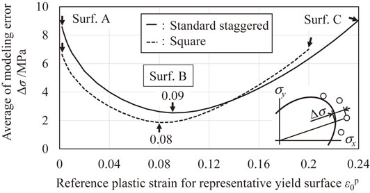
The representative yield surface in the surface interpolated differential hardening model described in Section 4.2 is determined in this section. Let the initial yield surface ($\varepsilon_{0}^{\text{p}} = 0.001$) be surface A, and let the yield surface of the maximum analysis range $\varepsilon_{0}^{\text{p}}$ (0.24 for the staggered arrangement, 0.20 for the square arrangement) be surface C. Surface B is placed between surfaces A and C, and the differential hardening is modeled with two sections and three surfaces.
Figure 6 shows the average value of the error between the differential hardening model and stress point on the contour of equal plastic work when the reference plastic strain $\varepsilon_{0}^{\text{p}}$ for surface B is varied. Both perforated sheet metals had minimum values when the reference plastic strain was slightly smaller than the middle of the approximated region. From this result, the representative yield surface B was set as the yield surface at $\varepsilon_{0}^{\text{p}} = 0.09$ for the staggered arrangement and $\varepsilon_{0}^{\text{p}} = 0.08$ for the square arrangement.
4.5 Approximation result of yield function
Using the modeling method described thus far, the approximated representative yield surface is shown in Fig. 3 with a thick solid line. In each hole arrangement, the in-plane anisotropy of the initial yield surface and tensile/compressive asymmetry of the subsequent yield surface were appropriately approximated. In addition, the surface interpolated by the differential hardening model is shown by the thin broken line in Fig. 3. The surface interpolation model can appropriately represent the stress points on the contour of the equal plastic work obtained by unit cell analysis.
5. Validation
Finally, to validate the model, the validity of the macro yield function model is confirmed by comparing the experimental results of the uniaxial tensile test and cylindrical deep drawing with the results of the finite element analysis using the macro model.
5.1 Validation by uniaxial tensile test
For the two types of perforated sheet metal, JIS 13 B specimens were cut at four angles θ from the c direction to the s direction, and a uniaxial tensile test was performed.
First, to validate the analysis of the homogenization method, Fig. 7 shows a comparison between the results of the experiment and the analysis of the shape of a hole at strain εx = 0.182 in the c and s directions. The ligament where deformation is concentrated differs depending on the tensile direction. Therefore, the deformed shape of the hole is different. In the analysis of the unit cell, the characteristic deformed shape of the hole can be reproduced.
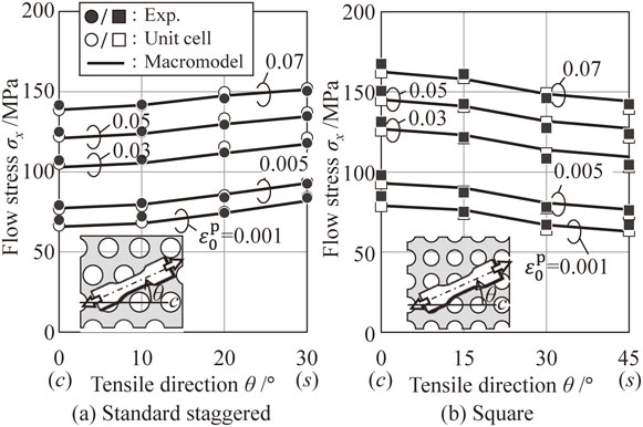
Figure 8 shows the in-plane distribution of the flow stress under uniaxial tension. The experimental values, values obtained by unit cell analysis, and values modelled by the macro yield function are shown. The modeled results properly expressed the characteristics of in-plane anisotropy.
Figure 9 shows the in-plane distribution of the apparent r-value in the uniaxial tensile test. The apparent r-value is defined by the following equation from the tensile direction strain εx and the width direction strain εy under uniaxial tension.
| \begin{equation}
r_{a} = -\frac{\varepsilon_{y}}{\varepsilon_{x} + \varepsilon_{y}}
\end{equation}
| (15) |
The perforated sheet metal does not satisfy the macroscopic constant volume condition. Therefore, this is described as an apparent value. Figure 9 shows the experimental results, unit cell analysis results, and model values of the macro yield function. The model value shows a slightly lower value at θ = 45° in a square arrangement. However, the macro model can express the characteristic tendency of deformation anisotropy.
5.2 Validation by cylindrical deep drawing
As shown in Fig. 3, in the two types of perforated sheet metals considered in this study, there is a remarkable difference in the yield surface when tension and compression are combined in the plane. This stress state is a specific state that occurs in the flange during the deep drawing process. Therefore, the validity of the macro model was evaluated using a cylindrical deep drawing test.
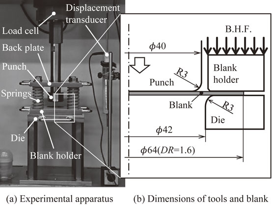
Figure 10 shows the appearance and dimensions of a simple deep-drawing experimental apparatus incorporated into a universal testing machine. A blank holding force was applied by springs built into the columns, and deep drawing was performed using a punch attached to the crosshead. A circular blank of ϕ64 mm was cut from two types of perforated sheet metal and drawn with a drawing ratio of 1.6.
In the finite element analysis, thin shell elements were used to model the blanks. To superpose multiple CPB2006 yield functions to express the rotational symmetry and incorporate the differential hardening model, the user subroutine library UMMDp for the anisotropic yield function was partially modified and used.22) In this analysis, the associated flow rule was used to calculate the direction of the plastic strain increment. Coulomb friction coefficient μ = 0.15 was set to be the friction between the tools and the blank.
Figure 11 shows a comparison of the appearance of the drawn cup shape. In the experiments, the staggered arrangement sheet exhibited almost no ears. However, the square arrangement sheet clearly shows four ears. This tendency can be appropriately predicted in the finite element analysis, as shown in the lower row of the figure. In addition, the deformation of the holes in the s and c directions of the square arrangement sheet is in good agreement with the deformation mode shown in Fig. 4. However, the pitch of the small wrinkles observed in the experimental results of the square arrangement was close to the dimensions of the unit cell. Therefore, the assumption of homogenization of material properties does not hold, and it cannot be predicted by analysis.
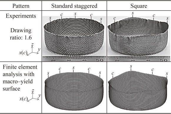
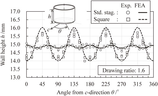
Figure 12 shows a quantitative comparison of ear heights. The ears of the staggered arranged sheet have slight peaks in the c direction and valleys in the s direction. In the square arrangement, there are valleys in the c direction and peaks in the s direction, and large ears exceeding 10% of the cup height are generated. For both hole arrangements, the ear shape can be appropriately predicted using the macro yield function model proposed in this study.
6. Conclusion
Numerical material tests using the homogenization method were performed on two types of perforated sheet metals with different hole arrangements, and the macro yield surface was modeled from the contour of equal plastic work of unit cell analysis. We also evaluated the validity of the proposed model by comparing it with the experimental results. The following conclusions were drawn:
-
(1)
The yield surface of the perforated sheet metal is strongly affected by the difference in the hole arrangement under the combined stress states of tension and compression. The subsequent yield surfaces show differential hardening and tension/compression asymmetry.
-
(2)
We proposed a method to introduce rotational symmetry to the yield surface, and the yield condition was modeled as the weighted sum of the CPB2006 yield function, which can consider tension/compression asymmetry. Differential hardening was modeled using the surface interpolation method.
-
(3)
We compared the analysis results of the modeled macro yield function and experimental results for the uniaxial tension and deep drawing tests. The analysis results for both perforated sheet metals showed good agreement with the experimental results. The effectiveness of the homogenization method on the modeling of plastic constitutive equation for sheet metal forming is demonstrated.
Acknowledgments
We would like to express our gratitude to Tomokage Inoue of Mechanical Design Co., Ltd., who provided advice regarding setting the analysis parameters for the deep drawing process.
REFERENCES
- 1) K. Terada and N. Kikuchi: Kinshitsukaho-Nyumon, (Maruzen, Tokyo, 2008) pp. 147–152.
- 2) N. Takano, Y. Uetsuji and T. Asai: Micro Mechanical Simulation, 67(102), (Corona Publishing Co., Tokyo, 2008).
- 3) K. Yamamoto, N. Hirayama and K. Terada: Trans. Jpn. Soc. Mech. Eng. 82 (2016) 16–00056.
- 4) A. Yamanaka, K. Hashimoto, J. Kawaguchi, T. Sakurai and T. Kuwabara: J. JILM 65 (2015) 561–567. doi:10.2464/jilm.65.561
- 5) H. Iseki, T. Murota and K. Kato: J. JSTP 30 (1989) 304–311.
- 6) H. Iseki, T. Murota, K. Kato and S. Hayashi: Trans. Jpn. Soc. Mech. Eng. Ser. A 55 (1989) 994–999. doi:10.1299/kikaia.55.994
- 7) T. Tatenami: J. JSTP 36 (1995) 671–676.
- 8) H. Khatam and M.-J. Pindera: Int. J. Plast. 27 (2011) 1537–1559. doi:10.1016/j.ijplas.2010.10.004
- 9) W.J. O’Donnell and J. Prowski: Trans. ASME, J. Appl. Mech. 40 (1973) 263–270. doi:10.1115/1.3422938
- 10) H. Takizawa and T. Sakai: J. JSTP 60 (2019) 262–267. doi:10.9773/sosei.60.262
- 11) H. Takizawa: Proc. 2014 Jpn. Spring Conf. Technol. Plast., (2014) pp. 343–344.
- 12) MSC Software: Marc 2014 Vol. D User Subroutines and Special Routines, 98–102.
- 13) F. Yoshida: Dansosei-Rikigaku-no-Kiso, (Kyoritsu Shuppan Publishing Co. LTD, 1997) p. 165.
- 14) R. Hill and J.W. Hutchinson: J. Appl. Mech. 59 (1992) S1. doi:10.1115/1.2899489
- 15) R. Hill, S.S. Hecker and M.G. Stout: Int. J. Solids Struct. 31 (1994) 2999–3021. doi:10.1016/0020-7683(94)90065-5
- 16) T. Kuwabara: J. JSTP 57 (2016) 934–939. doi:10.9773/sosei.57.934
- 17) O. Cazacu, B. Plunkett and F. Barlat: Int. J. Plast. 22 (2006) 1171–1194. doi:10.1016/j.ijplas.2005.06.001
- 18) R.K. Verma, T. Kuwabara, K. Chung and A. Haldar: Int. J. Plast. 27 (2011) 82–101. doi:10.1016/j.ijplas.2010.04.002
- 19) D. Yanaga, H. Takizawa and T. Kuwabara: J. JSTP 55 (2014) 55–61. doi:10.9773/sosei.55.55
- 20) B. Plunkett, R.A. Lebensohn, O. Cazacu and F. Barlat: Acta Mater. 54 (2006) 4159–4169. doi:10.1016/j.actamat.2006.05.009
- 21) F. Yoshida, H. Hamasaki and T. Uemori: Int. J. Plast. 75 (2015) 170–188. doi:10.1016/j.ijplas.2015.02.004
- 22) H. Takizawa, K. Oide, K. Suzuki, T. Yamanashi, T. Inoue, T. Ida, T. Nagai and T. Kuwabara: Proc. NUMISHEET 2018, (2018) 012099.
Appendix
The basic equations for incorporating the surface-interpolated differential hardening model used in this study into the finite element analysis code are explained in this appendix. The Voigt notation used in the explanation of the finite element method was adopted for mathematical description. Many finite element codes provide constitutive law subroutines with a hypoelastic model that allows any material model to be incorporated. In the hypoelastic subroutine, the stress {σn} at step n and the strain increment {Δε} from step n to n + 1 are given to solve the stress {σn+1} after the increment. Here, the backward Euler scheme used in the static implicit method is adopted.
A.1 Basic Formula of the Backward Euler Scheme
In the backward Euler scheme, the equations used for the constitutive law are satisfied after increment (n + 1). The relation that the stress {σn+1} after increment is on the differentially hardened yield surface is expressed by the following equation.
| \begin{equation}
\bar{\sigma}(\sigma_{n + 1},\bar{\varepsilon}_{n + 1}^{\text{p}}) - H(\bar{\varepsilon}_{\text{n} + 1}^{\text{p}}) = 0
\end{equation}
| (A.1) |
Here, $\bar{\varepsilon }_{n + 1}^{\text{p}} = \bar{\varepsilon }_{n}^{\text{p}} + \Delta \bar{\varepsilon }^{\text{p}}$ represents the equivalent plastic strain after the increment. $H(\bar{\varepsilon }^{\text{p}})$ represents the work-hardening function. An associated flow rule is assumed for the plastic strain increment {Δεp}, and is expressed by the following equation:
| \begin{equation}
\{\Delta\varepsilon^{\text{p}}\} = \Delta\bar{\varepsilon}^{\text{p}}\frac{\partial \bar{\sigma}}{\partial \{\sigma\}} \equiv \Delta \bar{\varepsilon}^{\text{p}}\{N_{n + 1}\}
\end{equation}
| (A.2) |
The partial derivative of the yield function with respect to the stress component is denoted as {N}. If the total strain increment {Δε} is decomposed to elastic and plastic parts in an additive form, the elastic strain increment {Δεe} can be expressed as follows:
| \begin{equation}
\{\Delta\varepsilon^{\text{e}}\} = \{\Delta\varepsilon\} - \{\Delta\varepsilon^{\text{p}}\}.
\end{equation}
| (A.3) |
From Hooke’s law, the stress increment {Δσ} is as follows:
| \begin{equation}
\{\Delta\sigma\} = [D^{\text{e}}]\{\Delta\varepsilon^{\text{e}}\}.
\end{equation}
| (A.4) |
Here, [De] is an elastic matrix. Using eqs. (A.3) and (A.4), the updated stress can be expressed as follows:
| \begin{align}
\{\sigma_{n + 1}\} &= \{\sigma_{n}\} + \{\Delta\sigma\} = \{\sigma_{n}\} + [D^{\text{e}}]\{\{\Delta\varepsilon\} - \{\Delta\varepsilon^{\text{p}}\}\}\\
& = \{\sigma^{\text{Try}}\} - \Delta \bar{\varepsilon}^{\text{p}}[D^{\text{e}}]\{N_{n + 1}\},
\end{align}
| (A.5) |
where {σ
Try} is a trial stress, assuming that {Δε} are all elastic.
A.2 Stress Integration
In stress integration, the equivalent plastic strain increment $\Delta \bar{\varepsilon }^{\text{p}}$ and stress increment {Δσ} that satisfy the nonlinear simultaneous equations shown in eqs. (A.1) and (A.5) are solved for the given {Δε}. Scalar function g1 and vector function {g2} are defined as the residual of eqs. (A.1) and (A.5).
| \begin{equation}
g_{1} = \bar{\sigma}(\sigma_{n} + \Delta \sigma,\bar{\varepsilon}_{n}^{\text{p}} + \Delta \bar{\varepsilon}^{\text{p}}) - H(\bar{\varepsilon}_{n}^{\text{p}} + \Delta \bar{\varepsilon}^{\text{p}})
\end{equation}
| (A.6) |
| \begin{equation}
\{g_{2}\} = \{\sigma_{n}\} + \{\Delta\sigma\} - \{\sigma^{\text{Try}}\} + [D^{\text{e}}]\Delta \bar{\varepsilon}^{\text{p}}\{N_{n + 1}\}
\end{equation}
| (A.7) |
The Newton–Raphson method was used to make these residual functions zero. Equations (A.6) and (A.7) are linearized, and the correction of unknown variables ({δΔσ} and $\delta \Delta \bar{\varepsilon }^{\text{p}}$) is solved by simultaneous equations. The correction $\delta \Delta \bar{\varepsilon }^{\text{p}}$ of the equivalent plastic strain increment can be obtained using the following equation:
| \begin{equation}
\delta \Delta \bar{\varepsilon}^{\text{p}} = \cfrac{g_{1} - \{N\}^{\text{T}}[E]^{-1}\{g_{2}\}}{\{N\}^{\text{T}}[E]^{-1}[D^{\text{e}}]\biggl\{\{N\} + \Delta \bar{\varepsilon}^{\text{p}}\cfrac{\partial\{N\}}{\partial \bar{\varepsilon}^{\text{p}}}\biggr\} - \cfrac{\partial \bar{\sigma}}{\partial \bar{\varepsilon}^{\text{p}}} + \cfrac{\partial H}{\partial \bar{\varepsilon}^{\text{p}}}}.
\end{equation}
| (A.8) |
Using [I] as the identity matrix, [E] is as follows:
| \begin{equation*}
[E] = [\text{I}] + \Delta \bar{\varepsilon}^{\text{p}}[D^{\text{e}}]\frac{\partial\{N\}}{\partial\{\sigma\}^{\text{T}}}.
\end{equation*}
|
From the correction $\delta \Delta \bar{\varepsilon }^{\text{p}}$, the correction of the stress increment is as follows:
| \begin{equation}
\{\delta \Delta \sigma\} = -[E]^{-1}\left\{\{g_{2}\} + [D^{\text{e}}]\left\{\{N\} + \Delta \bar{\varepsilon}^{\text{p}}\frac{\partial\{N\}}{\partial \bar{\varepsilon}^{\text{p}}}\right\}\delta \Delta \bar{\varepsilon}^{\text{p}}\right\}.
\end{equation}
| (A.9) |
Using eq. (A.9), with {Δσ} = [De]{Δεe} and $\Delta \bar{\varepsilon }^{\text{p}} = 0$ as the initial values, $\Delta \bar{\varepsilon }^{\text{p}}$ and {Δσ} are modified until the residual functions g1 and |{g2}| satisfy the convergence criteria.
A.3 Consistent Tangent Matrix
The static implicit procedure requires tangential stiffness, which is consistent with the stress integration algorithm. The consistent tangent matrix can be obtained by deriving the relationship between the perturbation of the strain increment {δΔε} and the perturbation of stress increment {δΔσ} from eqs. (A.1) and (A.5).
The following equation is obtained from the total derivative of eqs. (A.1) and (A.5), respectively.
| \begin{equation}
\{N\}^{\text{T}}\{\delta \Delta \sigma\} + \frac{\partial \bar{\sigma}}{\partial \bar{\varepsilon}^{\text{p}}}\delta \Delta \bar{\varepsilon}^{\text{p}} - \frac{\partial H}{\partial \bar{\varepsilon}^{\text{p}}}\delta \Delta \bar{\varepsilon}^{\text{p}} = 0
\end{equation}
| (A.10) |
| \begin{align}
&\{\delta \Delta \sigma\} = [D^{\text{e}}]\{\delta \Delta \varepsilon\} \\
&\quad - [D^{\text{e}}]\left\{\delta \Delta \bar{\varepsilon}^{\text{p}}\{N\} + \Delta \bar{\varepsilon}^{\text{p}}\frac{\partial \{N\}}{\partial \{\sigma\}^{\text{T}}}\{\delta \Delta \sigma\} + \Delta \bar{\varepsilon}^{\text{p}}\frac{\partial \{N\}}{\partial \bar{\varepsilon}^{\text{p}}}\delta \Delta \bar{\varepsilon}^{\text{p}}\right\}
\end{align}
| (A.11) |
Solving eq. (A.11) for {δΔσ}, establishes the following.
| \begin{equation}
\{\delta \Delta \sigma\} = [E]^{-1}[D^{\text{e}}]\left\{\{\delta \Delta \varepsilon\} - \left\{\{N\} + \Delta \bar{\varepsilon}^{\text{p}}\frac{\partial\{N\}}{\partial\{\sigma\}^{\text{T}}}\right\}\delta \Delta \bar{\varepsilon}^{\text{p}}\right\}
\end{equation}
| (A.12) |
Substituting eq. (A.12) into eq. (A.10) and solving for the $\delta \Delta \bar{\varepsilon }^{\text{p}}$, the following is obtained:
| \begin{equation}
\delta \Delta \bar{\varepsilon}^{\text{p}} = \cfrac{g_{1} - \{N\}^{\text{T}}[E]^{-1}[D^{\text{e}}]\{\delta \Delta \varepsilon\}}{\{N\}^{\text{T}}[E]^{-1}[D^{\text{e}}]\biggl\{\{N\} + \Delta \bar{\varepsilon}^{\text{p}}\cfrac{\partial\{N\}}{\partial \bar{\varepsilon}^{\text{p}}}\biggr\} - \cfrac{\partial \bar{\sigma}}{\partial \bar{\varepsilon}^{\text{p}}} + \cfrac{\partial H}{\partial \bar{\varepsilon}^{\text{p}}}}
\end{equation}
| (A.13) |
Finally, by substituting eq. (A.13) into eq. (A.12), a consistent tangent matrix can be obtained by the following equation:
| \begin{equation}
\{\delta \Delta \sigma\} = \left[\cfrac{[e]\biggl\{\{N\} + \Delta \bar{\varepsilon}^{\text{p}}\cfrac{\partial\{N\}}{\partial \bar{\varepsilon}^{\text{p}}}\biggr\}\{N\}^{\text{T}}[e]}{\{N\}^{\text{T}}[e]\biggl\{\{N\} + \Delta \bar{\varepsilon}^{\text{p}}\cfrac{\partial \{N\}}{\partial \bar{\varepsilon}^{\text{p}}}\biggr\} - \cfrac{\partial \bar{\sigma}}{\partial \bar{\varepsilon}^{\text{p}}} + \cfrac{\partial H}{\partial \bar{\varepsilon}^{\text{p}}}}\right]\{\delta \Delta \varepsilon\}
\end{equation}
| (A.14) |
Here, [e] = [E]−1[De]. The term $\{ \{ N\} + \Delta \bar{\varepsilon }^{\text{p}}(\partial \{ N\} /\partial \bar{\varepsilon }^{\text{p}})\} \{ N\}^{\text{T}}$ in the numerator of the consistent tangent matrix is asymmetric. Therefore, in the differential hardening model, the consistent tangent matrix is not a symmetric matrix.
A.4 Representation of Surface Interpolated Differential Hardening Model
In the surface-interpolated differential hardening model used in this study, the following equation was adopted:
| \begin{equation}
\bar{\sigma}(\sigma_{ij},\bar{\varepsilon}^{\text{p}}) = \mu (\bar{\varepsilon}^{\text{p}})\bar{\sigma}_{\text{A}}(\sigma_{ij}) + (1 - \mu(\bar{\varepsilon}^{\text{p}}))\bar{\sigma}_{\text{B}}(\sigma_{ij})
\end{equation}
| (A.15) |
| \begin{equation}
H(\bar{\varepsilon}^{\text{p}}) = \mu (\bar{\varepsilon}^{\text{p}})H(\bar{\varepsilon}_{\text{A}}^{\text{p}}) + (1 - \mu (\bar{\varepsilon}^{\text{p}}))H(\bar{\varepsilon}_{\text{B}}^{\text{p}})
\end{equation}
| (A.16) |
| \begin{equation}
\mu (\bar{\varepsilon}^{\text{p}}) = 1 - \frac{H(\bar{\varepsilon}^{\text{p}}) - H(\bar{\varepsilon}_{\text{A}}^{\text{p}})}{H(\bar{\varepsilon}_{\text{B}}^{\text{p}}) - H(\bar{\varepsilon}_{\text{A}}^{\text{p}})}
\end{equation}
| (A.17) |
Using eqs. (A.15)–(A.17), the variables specific to the differential hardening model used in the stress integration and the consistent tangent matrix can be easily calculated as follows:
| \begin{equation}
\frac{\partial \bar{\sigma}}{\partial \bar{\varepsilon}^{\text{p}}} = \frac{\partial\mu}{\partial \bar{\varepsilon}^{\text{p}}}(\bar{\sigma}_{\text{A}} - \bar{\sigma}_{\text{B}})
\end{equation}
| (A.18) |
| \begin{equation}
\frac{\partial \{N\}}{\partial \bar{\varepsilon}^{\text{p}}} = \frac{\partial\mu}{\partial \bar{\varepsilon}^{\text{p}}}\left(\frac{\partial \bar{\sigma}_{\text{A}}}{\partial \{\sigma\}} - \frac{\partial \bar{\sigma}_{\text{B}}}{\partial \{\sigma\}}\right)
\end{equation}
| (A.19) |
Here,
| \begin{equation}
\frac{\partial\mu}{\partial \bar{\varepsilon}^{\text{p}}} = \frac{-1}{H(\bar{\varepsilon}_{\text{B}}^{\text{p}}) - H(\bar{\varepsilon}_{\text{A}}^{\text{p}})} \cdot \frac{\partial H}{\partial \bar{\varepsilon}^{p}}
\end{equation}
| (A.20) |
The CPB2006 yield function proposed by Cazacu et al. is an anisotropic yield function that can express the SD effect. Here, we show the degenerate equation for the plane stress state for thin shell elements.
First, the deviation stress {S} is defined as
| \begin{equation}
\begin{Bmatrix}
S_{xx}\\
S_{yy}\\
S_{zz}\\
S_{xy}
\end{Bmatrix}
=
\frac{1}{3}
\begin{bmatrix}
2 & -1 & -1 & 0\\
& 2 & -1 & 0\\
& & 2 & 0\\
\textit{Sym.} & & & 3
\end{bmatrix}
\begin{Bmatrix}
\sigma_{x}\\
\sigma_{y}\\
0\\
\tau_{xy}
\end{Bmatrix}
.
\end{equation}
| (A.21) |
This {S} is linearly transformed by the following equation.
| \begin{equation}
\begin{Bmatrix}
\varSigma_{xx}\\
\varSigma_{yy}\\
\varSigma_{zz}\\
\varSigma_{xy}
\end{Bmatrix}
=
\begin{bmatrix}
C_{11} & C_{12} & C_{13} & 0\\
C_{12} & C_{22} & C_{23} & 0\\
C_{13} & C_{23} & C_{33} & 0\\
0 & 0 & 0 & C_{66}
\end{bmatrix}
\begin{Bmatrix}
S_{xx}\\
S_{yy}\\
S_{zz}\\
S_{xy}
\end{Bmatrix}
\end{equation}
| (A.22) |
The principal values of this {Σ} are found and called Σ1, Σ2, and Σ3. Here, Σ3 = Σzz. Using the above equation, the CPB2006 yield function $\bar{\sigma }$ is expressed by the following equation.
| \begin{equation}
\bar{\sigma}^{a} = (|\varSigma_{1}| - k\varSigma_{1})^{a} + (|\varSigma_{2}| - k\varSigma_{2})^{a} + (|\varSigma_{3}| - k\varSigma_{3})^{a}
\end{equation}
| (A.23) |
The parameters of the yield function to be determined are Cij, k, and a (a total of nine parameters). In this study, these parameters were determined by minimizing the sum of squares of the error with the stress point of equal plastic work.