Abstract
Mechanoluminescence (ML) materials, e.g., SrAl2O4:Eu2+, emit visible light when mechanical stress is applied. It was reported that the intensity of the light is in proportion to the applied von Mises stress. Therefore, acting von Mises stress can be measured from the intensity using a calibration curve. To make the ML measurements easier and more flexible, a detachable ML film has been newly developed. One surface of the base sheet was coated with detachable adhesive, while the other was coated with ∼5 µm thick ML layer. Two ML films were taken from one ML sheet so that the two pieces have identical ML properties. One piece was pasted on an A6061 aluminum alloy test piece (JIS13B, t = 1.0 mm) to obtain a calibration curve by the tensile test. The other piece was pasted on another A6061 test piece with a circular opening at the center to reveal the nonuniform stress distribution. The von Miese stress converted from the ML intensity showed a good agreement with the prediction by finite element analysis (FEA). It is concluded that the detachable ML film is sufficiently accurate and practical means to measure stress distribution in the target material.

1. Introduction
There are strong demands to visualize stress or strain distribution in loaded objects. The distribution is the most useful information to reveal mechanical stiffness and to improve product performance. The most popular and fundamental technique is the strain gauge technique; however, it detects local strains only at some fixed points.1–4)
To know an areal distribution directly, a pressure-sensitive film has been used.5) The film pasted on a test piece changes its color if the applied stress exceeds a certain stress threshold. This is due to the burst of micro bubbles including marker liquid under the pressure. Because of that, the film is unreversible and gives only the information about the applied stress is high or low to the threshold, so not suitable for quantitative measurement.
Recently, a digital image correlation (DIC) was rapidly developed as an advanced non-contact strain measurement technique.6–9) To obtain the strain distribution, the technique tracks an identical target point from two images which were taken after a time interval, and the stress distribution is converted from the strain using the Hooke’s law. However, it needs to measure small strain accurately to know stress by that method, but it is difficult for DIC due to the lower resolution. Considering applications to metals under plastic deformation or metal forming, a technique which enables to measure and visualize stress distribution is demanded.
Against these techniques, applying Mechanoluminescence (ML) material to visualize mechanical phenomenon is expected to resolve these problems. ML material, e.g., SrAl2O4:Eu2+, is known the material which can emit visible light (ML light) by applying mechanical stimuli.10,11) The material was invented by Xu et al. for a stress image sensor at the end of 1990s. First, they attempted piezoelectric materials to supply an electric power to an Electrochromic Display (ECD),12) then got an idea to take out not electric but light emission energy from the material (e.g., SrAl2O4) by doping substitutional cations (e.g., Eu) as emission centers.11,13–15) The emission performance of the material was improved by introducing artificial Schottky defects as trap sites of holes and electrons and optimizing of crystal structure system for high deformability.16,17)
Before the deformation, the ML material must be irradiated by the light with shorter wavelength than the ML light to accumulate the energy for ML emission. The irradiated light is absorbed at emission centers and generates holes and electrons, then charge carriers are activated and trapped in defects. The charge carriers which trapped at defects are excited and released to the valence band or the conduction band depending on the level of the mechanical stress, finally the charge carriers return to the ground state of the emission center with emitting ML light.11,13)
At the early stage in the material development, the property of ML light, i.e., the intensity of it increases in proportion to von Mises stress, which is a scalar amount proportional to the square root of elastic shear strain energy, was confirmed experimentally.18–20) Li et al. proved that the material enabled to visualize a quantitative mapping of von Miese stress as below experiments.18,19) First, a calibration curve, i.e., a relationship between stress and ML light intensity was obtained in a tensile test with a 120 µm thick ML layer coated on an A5052 aluminum alloy sheet. Secondly, a ML light image which was obtained with another specimen but having a hole at the center. As the specimen shows nonuniform strain and stress deformation, the ML intensity on the image was converted into the stress using the calibration curve. It was reported that these experimental results showed good agreement with those by the Finite Element Analysis (FEA).21)
Currently, the ML material is commercially available and considered for possible concrete applications in civil engineering.22) However, two major drawbacks exist, the one is how to fix the material onto the testing objects, and the other is the thickness optimization of the ML material layer which is associated with the particle size. Usually, a spray-painting technique was used to fix the ML material, which is a sort of ceramics, onto the testing object directly. However, it had difficulties in reliability and reproducibility in ML measurement, because the layer was too thick to achieve homogeneity and reproducibility. To overcome such problems and to improve ML image quality, the authors focused on the screen-printing technique using fine ground ML particle and succeeded to obtain ∼5 µm thick ML layer in the previous paper.23) As the result, Lüders band propagation in the test piece was visualized by the ML layer on the A1050 aluminum sheet.23)
As described above, the direct screen-printed ML layer may be suitable for applications to detect small stress change just like Lüders band phenomenon, however, the coating process to the testing object should be performed before every measurement. To improve flexibility and applicability of the ML measurements, a detachable ML film which was fabricated by printing ∼5 µm ML layer onto a one surface of resin base having detachable adhesive layer on the other surface, was studied. The ML measurement can be conducted by just putting the ML film onto the testing object. Furthermore, the film can be peeled off easily after the test. The property is expected to be practical to an industrial product inspection, for example.
Moreover, such a ML film has an advantage in quantitative measurement. Once ML sheet (i.e., larger one) is prepared, the smaller ML film pieces, which have identical ML performance because of the same origin, can be taken from the larger sheet, and the pieces can be allotted for either the calibration curve measurement or the ML analysis of the testing object. In addition, the elastic deformability of the film itself is also important. Namely, the system, where ML layer formed onto the testing object directly, is difficult to analyze stress state of the testing object in plastic region, but the system, of which ML layer is formed onto an elastic base, seems to be suitable to analyze because elasticity is maintained if the testing object starts to deform plastically.
The purposes of this study are as follows:
-
1.
To confirm the reproducibility of the previous study by Li et al.18,19) That is, to reconfirm the validity of the local stress converted with the calibration curve, which is the relationship between ML light intensity and von Mises stress. The tensile test with a thinner screen-printed ML layer than ever on an aluminum alloy test piece is conducted to check the accuracy of measurement.
-
2.
To extend industrial applications, the detachable ML sheet is produced and assessed. The usefulness and accuracy of the detachable sheet is discussed.
2. Experimental
2.1 Overview
Figure 1 shows an overview of this study. First, the ML sheet was prepared, and then the small pieces of films were cut off. In Experiment 1, a calibration curve was obtained by a tensile test with a ML measurement. A standard-shape test piece with the ML film on one surface was used as a specimen. In Experiment 2, another specimen having an opening hole at its center was used to cause stress distribution. First, the qualitative visualizing ability of the film was confirmed by the ML distribution showing typical stress distribution pattern of the hole opened test pieces. Secondly, the quantitative ability was evaluated by comparing the converted stress from ML intensity with the predicted von Mises stress by FEA under the same conditions.
2.2 Materials and Specimen
To attain detachable ability, a commercially available polyester sheet having a detachable adhesive layer (t = 59 µm, adhesive force: 0.25 N/25 mm: JIS Z 0237) on one surface was adopted as a base. As described above, the ML sheet was fabricated by forming ∼5 µm ML layer onto the other surface of the base against the detachable adhesive layer. The ML particles (ML-032, Sakai Chemical Industries Co. Ltd., Japan, D50 = 3.3 µm, D90 = 5.2 µm, Emission wave length: λ = 520–530 nm) were used, but applied additional grinding process with a jet mill to make particles finer (D50 = 1.6 µm, D90 = 2.1 µm) for pigments because the original particles of SrAl2O4 system, which synthesized by solid phase method, have a limitation to obtain sufficient intensity of emission.24) The paint for the screen-printing was prepared by mixing the fine ML particles and a transparent ink which was composed of urethane resin, hardener, and solvent. The ML layer was coated onto the base of A4 size: 210 × 297 mm with #500 stainless steel mesh by the screen-printing technique. It is the critical factor to use finer particles to form the thinnest layer than ever.23)
A JIS A6061P-T6 aluminum alloy sheet (t = 1.0 mm, Standard-test piece Co. Ltd., Japan) were used for experiments. The sheet was machined into JIS13B standard shape for tensile tests by the supplier. The objective of this study was to confirm the quantification ability of the ML film, then to establish a measuring technique of the stress distribution under loading conditions. To attain the above goal, a circle hole (4 mm diameter, at the center part of the test piece) was pierced by an additional machining on a normal test piece.
The test pieces with the ML films pasted by own adhesive ability were used as the specimens in this study.
2.3 Experimental procedure
The details of experiment in this study are illustrated in Fig. 2, which is also described in the previous paper.23) As shown in Fig. 2(a), the specimen, i.e., the ML film (12.5 × 80 mm), which was taken from the ML sheet, was pasted on the test piece manual by so as not to contain air bubbles between the ML film and the test piece. It is notable that the ML film was peeled off easily after the experiments without damages to the test piece.

Figure 2(b) is a schematic of the experimental system.23) The experimental system consisted of a universal testing machine (UTM: AG-Xplus SC + Software: Trapezium X, Shimadzu Corp., Japan), an industrial camera, two blue LEDs (λ = 470 nm) and two PCs for instruments controllers, and all instruments were installed under dark room conditions. Two blue light LEDs, which were facing one side of specimen, were mounted on each side of the industrial camera and inclined each optical axis to cross at the center of the specimen surface. The industrial camera converts light intensity, which was captured at each CCD elements, into electric signal as pixel value of 12 bits, and the pixel value is proportional to the amount of incident photons. A matrix consisted of all pixel values on the CCD element was stored into the control PC. Each pixel values were added 4 bits for convenience in later analysis and accumulated as 16 bits of Tagged Image File Format (TIFF) by the “in-house” software for measurement control and data acquisition (acquisition SW).
Figure 2(c) shows a typical experimental procedure. The ML measurement is basically a tensile test with taking the ML images of the specimen under dark room conditions, however it needs two special processes, i.e., “exciting process” and “quenching process”.
The exciting process is an energy accumulating process to the ML substance by irradiating shorter wavelength light than ML emitting light, however the process induces the ML material persistent but gradually decreasing luminescence (afterglow) which is regarded as background noise, then the authors have to wait duration as the quenching process till the afterglow to be stable. In this study, the specimen was irradiated with blue light for 60 s as the exciting process, and then kept under the dark conditions for 120 s as the quenching process, however specimen images were not taken in these processes because the background levels were almost same and stable under the same exciting and the quenching conditions.
After quenching process, ML measurements, i.e., the tensile test with taking specimen images, were held. The data set of the one measurement run consisted of the pre-defined amount of image files having interval time equal to exposure time. However, the observed ML light is imposed the background noise (represented as M in Fig. 2(c)), then it is preferable to remove the background noise components in a later analysis. To achieve the removing process, the data set of background noise only were needed, then the images were taken under the identical conditions without tensile test (represented an N in Fig. 2(c)) after series of M measurement.
For digitization of ML information, a “in-house” software for ML analysis (analysis SW), which was developed as a trial product by the authors, was used. After two groups of data sets, i.e., M and N were read into the analysis SW, First, the working image having ML information only (represented an W in Fig. 2(c)), was created by subtracting the image of N from that of M, which were taken at the same elapsed time. Secondly, proper Region of Interest (ROI) for each experiment were defined manually on the W, and the average of intensity within ROI was calculated for evaluation data of ML intensity.
2.4 Numerical analysis
To evaluate the quantitative property of the calibration curve between ML intensity and stress obtained from Experiment 1 as shown in Fig. 1, the stress distribution was predicted by the numerical analysis for a specimen with a hole. The linear static structural analysis was performed using the commercial FEA software package ANSYS 2021R1. The geometry, finite-element mesh, material properties used in the analysis are shown in Fig. 3(a) and Fig. 3(b). In consideration of the symmetry, the 1/8 model was used, and the grip sections were omitted. On the symmetry planes, boundary conditions with zero displacement in the normal direction were imposed (refer to Section 3.3). A load of 575 N was applied at the end to correspond to a tension of 2.3 kN. The multi-linear isotropic hardening law was used as the material property. Before the FEA, the true stress - true strain curve in Fig. 3(c) was obtained from tensile tests using an extensometer to measure strain accurately. The test was held at the crosshead speed of 16.7 µm/s (1 mm/min) to nominal strain of ε = 0.1. The Young’s modulus was set to 71 GPa obtained from these tests. On the other hand, 0.33 was set as a typical value for the Poisson’s ratio. Figure 3(c) also shows the elastic limit of the test piece is ∼280 MPa (3.5 kN/12.5 mm2).

3. Results
3.1 Basic performance of the ML film
First, to confirm properties of the ML film on the test piece, tensile tests (n = 7) in elastic region were repeated at the crosshead speed of 83 µm/s (5.0 mm/min) to the elastic limit of 280 MPa (3.5 kN/12.5 mm2). The exposure time of 500 ms was adopted and interval time between the former and the later exposure was negligible. In the analysis process, the ROI (12.5 × 8 mm) was defined at the center part of specimen image, and the average of pixel value within the ROI was adopted as the ML intensity.
Figure 4(a) shows the ML intensity: X plotted against elapsed time: t from the 2nd run to the 7th run in the 7 times of repeat tests. As explained in Fig. 2(c), all runs were repeated with the series of experimental procedure. Same as the others ML experiments, the 1st run tends to show different tendency because of gripping the specimen by UTM cramps, then the results of it were excluded. The plots tend to show a sigmoidal curve.22) The phenomenon is presumed that the material has a threshold of stress to emit the ML intensity in lower region and start to decrease accumulated energy for ML emission in higher region. The elapsed time synchronizes stress increasing, then ML intensity of the film expects to show nearly linear increase with the stress.

As for repeatability, all curves showed good agreement, and it means the ML film showed good followability to the test piece till reaching maximum load without detaching in the repeat tests. The above-mentioned results suggest that the ML film has sufficient properties for quantitative measurement.
To evaluate uniformity of the ML sheet, the three pieces of ML films as #1, #3 and #5 cut off from the inner part of one ML sheet because there was nonuniform part around outer part obviously by UV irradiation, and then ML measurements were held by the same method in Fig.4(a). The films were tested 4 times each, and then average data sets of #1, #3, #5 from 2nd to 4th runs were calculated. Figure 4(b) shows the ML intensity – time plots of them, no major difference was recognized between those plots. The average intensity at their peak intensities was 455.2, while the coefficient of variation was 4.256%. The result suggests that the ML sheet has fair uniformity. As for accuracy, the resolution of CCD camera was 12 bits, in contrast the peak intensity of 455.2 can be expressed by 9 bits, then sufficient accuracy was obtained in this study.
3.2 Calibration curve for quantitative analysis
Two data acquisition were held in a same ML measurement including a tensile test to obtain a stress - ML intensity curve as a calibration curve which convert pixel value from ML intensity in a tiff image file into stress. The ML film pasted on a normal test piece was used for the measurement. The experiment conditions were the crosshead speed at 83 µm/s (5 mm/min) to 240 MPa (3.0 kN/12.5 mm2), exposure time of 500 ms for taking ML image. Tests were repeated six times continuously. The first half of the tests were held for accumulating ML intensity with elapsed time with the acquisition SW, and the latter half were held for accumulating stress with elapsed time with the Trapezium X software. Considering the repeatability shown in Fig. 4(a), the data sets from the 3rd run of each test groups were adopted to determine the calibration curve. The relationship between ML intensity and time, which is shown in Fig. 5(a), was obtained by the same procedure in the section 3.1 shows sigmoidal curve as described in Fig. 4, and relation between stress and time in Fig. 5(b) was nearly linear. These data sets were converted into Comma-Separated Values (CSV) format file by each software function, and then plotted the ML intensity against stress within the Microsoft office EXCEL software.

Figure 6(a) shows ML intensity: X (pixel value) against stress: σ (MPa) using all data sets obtained from the experiments. There are two inflection points, which are derived from ML property, then third-order polynomial regression was applied to obtain the calibration curve using function of Microsoft Excel software. Equation (1) and its coefficient of determination: R2 was 0.9906 was obtained as a calibration equation at the same time.
| \begin{equation}
\sigma = 9.658\times 10^{-6} X^{3} - 5.264\times 10^{-3} X^{2} + 1.282X + 23.28
\end{equation}
| (1) |
On the other hand, the curvature at lower inflection point was remarkable because of the threshold as described, and plots using data set in the region over ML intensity of 50 shows nearly straight as shown in Fig. 6(b). Then, linear regression applied to the data set of Fig. 6(b), and eq. (2) and its coefficient of determination: R2 was 0.9848 was obtained as optional regression equation.
| \begin{equation}
\sigma = 0.510X + 48.706
\end{equation}
| (2) |
Judging from R2, eq. (1) shows slight better regression than eq. (2).
3.3 Visualization of stress distribution
Li et al. proved that the ML light intensity shows good agreement with von Mises stress with a hole opened specimen, where well known and analytical solutions were presented to cause the stress distribution, by comparing the experimental results to FEA results.18,19) Same evaluation method was adopted to confirm the quantitative ability of the ML film.
As shown Experiment 2 in Fig. 1, the specimen consisted of the ML film and the test piece but having 4 mm hole in diameter at the center of it was used. Since the cross-sectional area along the horizontal center line was two-third to that of the normal test piece, then the maximum load in the experiment was determined 2.3 kN (3.5 kN × 2/3) not to exceed elasticity limit. The ML measurement was examined three times and one time of background noise acquisition was held, and the data of the 3rd run was adopted for the evaluation. The testing conditions of tensile test were the crosshead speed at 83 µm/s (5 mm/min) to 2.3 kN, exposure time of 500 ms for taking ML image.
4. Discussion
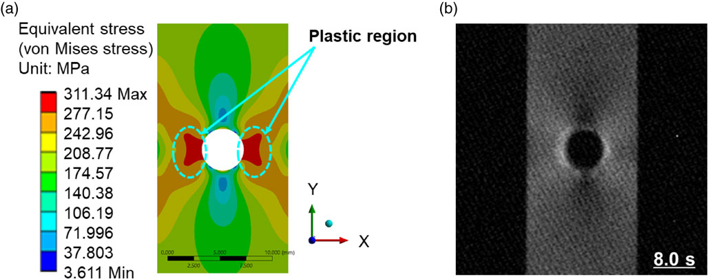
Figure 7 compares stress distribution patterns of same hole pierced specimen under the same conditions of loading at 2.3 kN. Figure 7(a) shows predicted von Mises stress distribution by FEA, and Fig. 7(b) shows the ML distribution, which was attributed to ununiform stress distribution from the real specimen. Both show similar patterns and stress concentrations at the horizontal sides around the hole. From the FEA results, it can be seen that the stress concentration regions are plastically deformed. As described above, qualitative agreement was confirmed between the two systems.
To evaluate the quantitative ability of the ML film, the measured stress, which was converted from ML intensity by the calibration equation, and the predicted von Miese stress (predicted stress) by FEA were compared at five reference points which were defined at the coordinates of #1: (−4, 0), #2: (−4, 4), #3: (−4, 8), #4: (0, 4) and #5: (0, 8) in mm from the hole center (0, 0). The predicted stresses were read out directly from ANSYS software.
As for the measured stress, first, TIFF images of ML were read into analysis SW, and ROI having 1 × 1 mm square, of which centers were coincided at the reference points #1–#5, were defined as ROI-n (n = 1–5), and then subtraction process was held to eliminate background noise, finally the averages within each ROIs were calculated. The data sets of ML intensity from each ROIs were converted into the stress by calibration equations and plotted against elapsed time. The data sets converted by eq. (1): third-order regression equation are shown in Fig. 8(a), by eq. (2): linear regression equation in Fig. 8(b), and both figures were superimposed with von Mises stress (predicted stress) by FEA for comparison. As is clear from the two figures, the measured stress by the third-order regression calibration equation shows better accordance to predicted stress than by the linear regression because it is omitted information in lower region is omitted in the regression. The accordance between two kinds of stress means that the ML intensity at any position in specimen enable to trace the local stress at any elapsed time.

To evaluate quantitatively, two kinds of measured stress around the maximum load point plotted against predicted stress at the same point, i.e., the average of measured stress between 8.0 ± 0.5 s at each ROIs was for the former, the von Mises stress at 2.3 kN at each reference points was for the later. As shown in Fig. 9, the predicted stress tends to underestimate the measured stress, but deviations almost are less than 10%, except for #1 vs. ROI-1. The result suggests a good agreement will be obtained with either method in elastic region in the others of applications. Two factors are presumed for the higher deviation between #1 and ROI-1 as below.

-
(1)
Plastically region: #1 was confirmed that was in plastically deformed region by FEA, then the calibration equations which were obtained in elastic region, were not applicable to such a deformation.
-
(2)
Attributed to the ROI scale: the gradient of stress was so acute, then defined ROI region to calculate average value was too large to calculate pinpoint value just as FEA.
In either case, it needs further investigation to increase accuracy by the proposed technique in higher stress region, especially for plastically region.
As for superiority between the third-order regression and the linear regression, there was no obvious difference, but the later showed better agreement than former. There is a low intensity and unstable region around the threshold to rising ML emission, then the third-regression equation including such information may be affected to calculate correct value. However, the ML film and the proposed technique showed sufficient performance to apply quantitative measurement.
5. Conclusion
To widen applications of mechanoluminescence (ML) material, a detachable ML film was fabricated by screen-printing ML layer on a surface of a resin sheet having a detachable adhesive layer on the other surface. The stress measurement performance of the film were evaluated with A6061 aluminum alloy test piece in tensile tests. Following remarks were obtained.
-
(1)
ML intensity was confirmed to increase with applied stress in the elastic region, In addition, the repeated tensile tests revealed that the relationship between the measured ML intensity and the applied stress was reproducible.
-
(2)
A test piece with a hole at the center, as a nonuniform elastic deforming system, was also stretched. The observed ML pattern qualitatively agreed with the distribution of von Mises stress predicted by the finite element method even in this film pasted specimen.
-
(3)
At some reference points on the tensile specimen with a hole, the stress was converted from the measured ML intensity using the relationship between ML intensity and stress, which was predetermined by tensile test of test pieces without hole, as a calibration curve. The converted stress showed good agreement with the prediction by the FE analysis. The discrepancy between the converted and the predicted was found to be less than 10%.
As the detachable ML film can be pasted at any places on most objects, it could be a practical device for quantitative stress measurement in industries.
REFERENCES
- 1) H. Fujita and T. Tabata: Acta Metall. 25 (1977) 793–800. doi:10.1016/0001-6160(77)90094-3
- 2) Y. Nakayama, K. Nomura and M. Furuta: J. JILM 56 (2006) 39–44. doi:10.2464/jilm.56.39
- 3) R. Onodera, M. Nonomura and M. Aramaki: J. Japan Inst. Metals 64 (2000) 1162–1171. doi:10.2320/jinstmet1952.64.12_1162
- 4) Y. Nakayama and M. Maeda: J. JILM 61 (2011) 240–245. doi:10.2464/jilm.61.240
- 5) A.B. Liggins, W.R. Hardie and J.B. Finlay: Exp. Mech. 35 (1995) 166–173. doi:10.1007/BF02326476
- 6) H. Tsuneishi, H. Taguchi, K. Morino, A. Yatsuhashi, K. Ikeda and S. Miyake: J. Jpn. Soc. Exp. Mech. 15 (2015) 277–281. doi:10.11395/jjsem.15.277
- 7) J. Zhang, M. Huang, B. Sun, B. Zhang, R. Ding, C. Luo, W. Zeng, C. Zhang, Z. Yang, S. van der Zwaag and H. Chen: Scr. Mater. 190 (2021) 32–37. doi:10.1016/j.scriptamat.2020.08.025
- 8) J. Ma, H. Liu, Q. Lu, Y. Zhong, L. Wang and Y. Shen: Scr. Mater. 169 (2019) 1–5. doi:10.1016/j.scriptamat.2019.04.044
- 9) H. Ait-Amokhtar and C. Fressengeas: Acta Mater. 58 (2010) 1342–1349. doi:10.1016/j.actamat.2009.10.038
- 10) C.N. Xu, T. Watanabe, M. Akiyama and X.G. Zheng: Appl. Phys. Lett. 74 (1999) 1236–1238. doi:10.1063/1.123510
- 11) C.N. Xu, T. Watanabe, M. Akiyama and X.G. Zheng: Appl. Phys. Lett. 74 (1999) 2414–2416. doi:10.1063/1.123865
- 12) C.N. Xu, M. Akiyama, P. Sun and T. Watanabe: Appl. Phys. Lett. 70 (1997) 1639–1640. doi:10.1063/1.118654
- 13) C.N. Xu: Encyclopedia of Smart Materials, Vol. 1, (John Wiley & Sons Inc., New York, 2002) pp. 190–201.
- 14) T. Matsuzawa, Y. Aoki, N. Takeuchi and Y. Murayama: J. Electrochem. Soc. 143 (1996) 2670–2673. doi:10.1149/1.1837067
- 15) F. Clabau, X. Rocquefelte, S. Jobic, P. Deniard, M.-H. Whangbo, A. Garcia and T.L. Mercier: Chem. Mater. 17 (2005) 3904–3912. doi:10.1021/cm050763r
- 16) M.V.S. Rezende, R.M. Araujo, M.E.G. Valerio and R.A.J. Jackson: J. Phys. Conf. Ser. 249 (2010) 012042. doi:10.1088/1742-6596/249/1/012042
- 17) C.N. Xu, H. Yamada, X. Wang and X.G. Zheng: Appl. Phys. Lett. 84 (2004) 3040–3042. doi:10.1063/1.1705716
- 18) C. Li, C.N. Xu, Y. Imai and N. Bu: Strain 47 (2011) 483–488. doi:10.1111/j.1475-1305.2009.00713.x
- 19) C. Li, C.N. Xu, L. Zhang, H. Yamada and Y. Imai: J. Vis. 11 (2008) 329–335. doi:10.1007/BF03182201
- 20) C.N. Xu: Ceramics Japan 44 (2009) 154–160.
- 21) O.C. Zienkiewicz, R.L. Taylor and J.Z. Zhu: The Finite Element Method: Its Basis and Fundamentals, 6th ed., (Elsevier Butterworth Heinemann, Burlington, 2005).
- 22) Y. Fujio, C.N. Xu, Y. Sakata, N. Ueno and N. Terasaki: J. Alloy. Compd. 832 (2020) 154900. doi:10.1016/j.jallcom.2020.154900
- 23) K. Kanamaru and H. Utsunomiya: Scr. Mater. 209 (2022) 114388. doi:10.1016/j.scriptamat.2021.114388
- 24) M. Kuboyama, H. Furusawa, D. Mori, Y. Takeda, O. Yamamoto, K. Asahino, K. Kamiya and N. Imanishi: J. Jpn. Soc. Powder Powder Metallurgy 65 (2018) 176–182. doi:10.2497/jjspm.65.176


