Abstract
In modern life, we are surrounded by and filled with electromagnetic noise caused by the dominant use of energy in the form of electricity. This situation is brought about by the fact that the noise is not understood theoretically. A new practice of noise reduction was introduced for the construction of Heavy Ion Medical Accelerator in Chiba (HIMAC). The key concept is a symmetric three-line circuit that arranges power supplies, noise filters and magnets around a third central ground line. A continuous theoretical effort forced us to find a new circuit theory involving a multiconductor transmission-line system starting from Maxwell’s equations without any approximation. We discuss the essence of all of these experimental and theoretical developments with the hope to remove unnecessary electromagnetic noise not only from power supplies, but also from all electric devices. The newly derived circuit theory of multiconductor transmission lines is universal, and establishes the validity of the practice of noise reduction.
I. Introduction
Electricity is the most convenient form of energy in modern life. Our circumstances (environment) are necessarily filled with electromagnetic noise emitted from all types of electric devices. Particularly in recent years, the use of the Insulated Gate Bipolar Transistor (IGBT) and the Metal Oxide Semiconductor-Field Effect Transistor (MOS-FET), the modern chopping devices of rectifiers, causes high-frequency noise to travel through electric circuits, and at the same time to go out to the environment freely. As a consequence, all electric devices should be used under the electromagnetic compatibility (EMC) rule. The problem that causes this situation is that there is no theoretical framework to clearly define electromagnetic noise in circuit theory.
At the frontier of particle accelerators, particularly synchrotrons using time-dependent magnetic fields, we cannot tolerate the usual amount of electromagnetic noise. In an effort to reduce the noise level in the cooler synchrotron TARN2, which was built and commissioned at the Institute for Nuclear Study of the University of Tokyo, one of the authors (K.S.) found a huge amount of noise in the conventional two-line circuit, where noise current flows through the surrounding materials such as the ground.1) This fact indicates that we should carefully consider the environment of any electric device for the stable operation of accelerators. Hence, for the construction of the Heavy Ion Medical Accelerator in Chiba (HIMAC), a careful theoretical study of a three-line circuit system was made based on lumped-parameter circuit theory. Consequently, a symmetric three-line (S3L) circuit system was constructed for the power supply, noise filter and a chain of magnets for the synchrotron with a third hard-wired central ground line.1),2)
We show in Fig. 1 a schematic diagram of the S3L circuit, which includes a power supply, noise filter and magnet system constructed for HIMAC, which turned out to work very stably with ultra-low noise. The S3L circuit is a new concept of noise reduction, which is not at all known within the community. In order to understand the performance of the HIMAC system, we studied theoretically the role of the S3L circuit used to reduce the noise in the magnets for the accelerators.3) The key concept is the use of both the normal (differential) and common (summed) modes. In a conventional two-line circuit, one usually uses the normal mode, where the normal-mode current is $I_{n} = \tfrac{1}{2}(I_{1} - I_{2})$ with $I_{1}$ and $I_{2}$ being the currents of lines 1 and 2. With the condition that the system is closed, $I_{1} + I_{2} = 0$, the normal-mode current is the current going through line 1, $I_{n} = I_{1}$. However, we have to consider other factors, such as the ground, since unexpected noises are caused by the coupling of the two-line circuit to the circumstances (environment) around it. A third line has to be included to represent these circumstances, which are electromagnetically connected to the two-line circuit. In this case, the summed current is not zero, $I_{1} + I_{2} \ne 0$. The common-mode current is then defined as $I_{c} = \tfrac{1}{2}(I_{1} + I_{2} - I_{3})$ using the third-line current, $I_{3}$. The common-mode current goes through the main two-lines and the third line. With the condition that the total current is zero, $I_{1} + I_{2} + I_{3} = 0$, in the case of no radiation the common-mode current is $I_{c} = I_{1} + I_{2} = - I_{3}$, which represents the summed current of the two main lines.
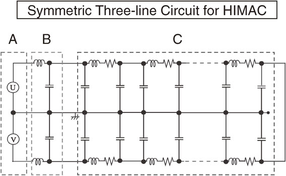
Unless some special arrangement is introduced to a two-line circuit, the currents in the normal and common modes will couple with each other. However, with the inclusion of the third line, we are able to use it explicitly as the central line, and arrange all of the electric components symmetrically around the central line. This is the definition of a symmetric three-line (S3L) circuit with the central line in the middle of the two lines and the symmetric arrangement around it. In the S3L circuit, we are able to show that the normal-mode current decouples from the common-mode current. We were able further to introduce twin noise filters symmetrically to reduce high-frequency noises in both the normal and common modes, which are caused by the twin power supplies. The HIMAC system with the power supply, noise filter and magnet system, shown in Fig. 1, is one example of the S3L circuit.
Electromagnetic noise usually has high-frequency components caused by a high frequency switching device of the power supply. Hence, we needed to study the performance of three-conductor transmission lines using a multi-conductor transmission-line (MTL) theory. We immediately found that the existing MTL theory is not suited to discuss the performance of the normal and common modes.4) To this end, we had to modify the differential equations including the coefficients of the capacitance, C, and express the potentials (voltages) in terms of the currents. In these new differential equations, there appeared other coefficients, named as the coefficients of potential P.4),5) In this case, we can use the condition of the total current being zero almost trivially. In the case where the currents are expressed in terms of voltages using C, this condition for the total current provides complicated expressions for all of the quantities, and eventually for the normal- and common-mode quantities.4) With the coefficients of potential P, we are able to treat the electromagnetic noise in the normal and common modes analytically, and clearly find the conditions for noise reduction.6)
We are aware that when conduction noise appears in an electric circuit along transmission lines, we experience the appearance of radiation noise from the transmission lines simultaneously. This fact suggested that we can study the radiation noise in addition to the conduction noise in a three-conductor transmission-line system. The radiation noise is related to a finite total current of $I_{1} + I_{2} + I_{3} \ne 0$, which is treated as an extra mode in a MTL system. We name this as the antenna mode, which is defined for the first time in terms of the potential, itself, while the normal and common modes are defined in terms of the potential difference, namely the voltage, similar to those of the conventional MTL theory. To this end, we had to introduce retarded potentials consisting of scalar and vector potentials to treat the radiation from a MTL system. The retarded potentials have both real and imaginary parts when expressed for a fixed frequency wave, namely, Alternating Current (AC). The real part has a singular behavior in the integrand for the retarded potential, and naturally provides transmission-line differential equations with coefficients of both the inductance and the potential in a natural manner. On the other hand, the imaginary part has the same phase as the resistance of conductors, and provides the effect of both the emission and absorption of electromagnetic waves in non-local integral forms. We were able to derive coupled (integro-) differential equations for the normal, common and antenna modes from Maxwell’s equations without introducing any approximation.7) With the new circuit theory of the MTL system, we conclude that only a S3L circuit can decouple the normal mode from the common and antenna modes, and can thus reduce the electromagnetic noise in an electric circuit.
After constructing new coupled MTL differential equations, we are able to suggest an ideal electric circuit used to expressly reduce conduction and radiation noises. It is very important to use a three-line circuit and to arrange all of the electric components symmetrically around the central ground line. The new circuit theory justifies the use of the HIMAC-type power supply, noise filter and magnet system for accelerators. Of course, the use of this S3L circuit should not be limited to accelerators, and should be applicable in all electric devices for good and stable operation to reduce the noise level. We further provide a supplementary statement that a common-mode noise in a conventional two-line circuit goes through the ground (circumstances) as an invisible signal. This invisible noise cannot be suppressed, in principle, by any commercial products, such as the common-mode choke and ferrite core for the two-line circuit. Thus, the invisible noise not only deteriorates the performance of the electric circuit, but also often breaks circuit components.
In this paper, we shall describe the development of a new circuit theory starting from a new practice involving an S3L circuit. The present study provides strict mathematical expressions for the common, normal, and antenna modes of a three-line system so as to clearly quantify such obscure knowledge in electric engineering as unbalanced and balanced circuits for the discussion of noise. In Sect. 2, we describe the observation of a common-mode noise in a conventional two-line circuit experimentally. This observation led us to consider a three-line circuit for the problem of electromagnetic noise. We then discuss an S3L circuit as a power supply, noise filter and magnet system of HIMAC. In Sect. 3, we introduce the concept of the normal and common modes using the lumped-parameter circuit theory. In Sect. 4, we consider a MTL theory that treats the normal and common modes by introducing coefficients of potential in place of coefficients of capacitance. In Sect. 5, we introduce a new circuit theory including the antenna mode starting from Maxwell’s equations. In Sect. 6, we discuss an ideal symmetric three-line circuit that can be used to reduce the noise due to the circumstances. We describe here actual cases involving a three-line circuit for HIMAC, J-PARC/MR and the well-known battery problem of the Boeing 787. We make a comment on the basic electromagnetism in view of the new circuit theory. In Sect. 7, we summarize the present study.
II. Common mode and practice of a symmetric three-line circuit
The first encounter of one of the authors (K.S.) to a symmetric three-line circuit for a chain of magnets was a drawing by Regenstreif for the proton synchrotron (CERN-PS) of the European Organization for Nuclear Research.2) This drawing of the CERN-PS magnet system corresponds to the magnet part of HIMAC, shown in Fig. 1. By studying the performance of the symmetric three-line circuit for a chain of magnets, it became clear that the common-mode noise should be suppressed by the operation of a chain of magnets. Following this concept, he designed a power supply, noise filter and magnet complex for HIMAC. This was the first time to use a symmetric three-line circuit in an accelerator, because the drawing of Regenstreif was not realized in CERN-PS. The concept of the symmetric arrangement was used only recently in CERN for the LHC accelerator. In the electric circuit for the power supply, noise filter and magnet system of HIMAC, as shown in Fig. 1, two points are very original in addition to the symmetrically arranged magnet part. One is the use of symmetrized twin power supplies made of thyristor semi-conductors. The twin power supplies produce noises both in the normal and common modes, which are confined in the three-line circuit. The twin power supplies made it possible to introduce filtering circuits symmetrically around the third line for noise reduction. The twin filters are able to almost completely reduce high-frequency noises in both the normal and common modes.3)
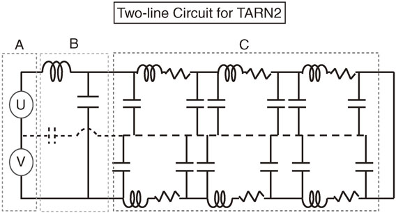
At the time of constructing the HIMAC power supply and magnet complex, K.S. encountered interesting experimental data involving a synchrotron cooler ring, TARN2, at Institute for Nuclear Study (INS) of the University of Tokyo, where a chain of magnets were arranged successively without considering the symmetrization, as shown in Fig. 2.8) This power and magnet circuit was in principle a two-line circuit, where the ground was never considered to be an electric line in the system. Here, there was no consideration of symmetrization of the arrangement of magnets in a two-line circuit. The bodies of all the magnets were connected to the ground, indicated by the dashed line. The ground has a conducting property, as we indicate by the dashed line in the figure. The twin power supplies with the switching device produce noises in both the normal and common modes. The noise in the normal mode goes through the two-line circuit, and can be reduced by a noise filter. On the other hand, the noise in the common mode goes through the ground, which is indicated by the dashed line with a stray capacitance. This means that even if there is no explicit connection between the middle point and the ground, the gap between the ground and the middle point functions as a capacitance.
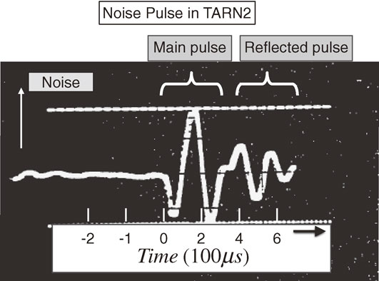
Although the noise filter was installed as shown in Fig. 2, there was a huge amount of noise in the magnets of TARN2, detected as shown in Fig. 3. The level of the noise was about $\Delta I/I_{DC} \sim 5 \times 10^{ - 3}$, which is the ratio of the current fluctuation to the DC excitation current ($I_{DC} = 200$ A in this operation) of the magnet coil. This large fluctuation was fatal for operating the TARN2 synchrotron. This noise pulse having a period of 195 µs appeared as a main component, while an associated smaller noise pulse due to reflection appeared slightly later by 267 µs with a period 200 µs. The phase of the reflected (associated) noise pulse was opposite to that of the main component. This fact indicated that the reflected noise wave was caused by the open end of the TARN2 power supply and magnet system. Hence, this noise should be related to the common mode, since for the normal mode the two-line circuit had a closed end, as can be seen in Fig. 2. This seemed to indicate that the ground line shown by the dashed line in Fig. 2 carried the noise pulse. Additionally, the signs of the noise pulses of the first magnet and the last magnet were found to be opposite. These two observations indicated that the noise pulses propagated through the environment (ground). Hence, the ground of the TARN2 circuit was acting as the third line of a three-line circuit. This was the first time to identify the property of noise due to the common mode. A large amount of noise went through the circumstance (ground). This noise was reduced by a factor of 4 by using a bridge resistance (50 Ω) of each coil of all the magnets of TARN2.2) However, we had to understand even more in order to construct a better power supply, noise filter and magnet system for realizing stable operation of HIMAC.
It was an important finding that the noise pulse from the power supplies arises not from the normal electric circuit, but from the environment (ground). It seems that the noise in the normal mode from the twin power supplies is reduced largely by a filtering device placed just after the twin power supplies. On the other hand, there is no device used to cut down the noise in the common mode in TARN2. Clearly, a reduction of noise has to be made for the noise in the common mode. K.S. therefore introduced twin noise filters for the power supply and magnet complex of HIMAC by taking the middle point of the twin power supplies connected in series and the third hard-wired central ground line, as shown in Fig. 1. These twin noise filters in the S3L circuit reduced noises both in the normal and common modes, and were able to reduce the noise level to about $\Delta I/I_{DC} \sim 10^{ - 6}$ as compared to $10^{ - 3}$ in the conventional method, which guaranteed stable operation of HIMAC. Here, the circumstances (environment) no longer affect the noise performance of the S3L circuit, although the ground seems to be the fourth line of the S3L circuit. The concept of the S3L circuit was also recently found by the power-supply group of CERN without any circuit theory, and it was actually applied to the LHC synchrotron in CERN.
III. Normal and common modes in a simple lumped-parameter circuit
We show here the reason for using the S3L electric circuit used to reduce noise in the common mode. In order to understand the HIMAC performance, we first consider a simple three-line lumped-parameter circuit, and introduce the concept of the normal and common modes. It is important to recognize that a conventional two-line electric circuit uses the normal mode, and that engineers design an electric circuit for their purpose in the most efficient and economical way by reducing possible noise in the normal mode. The TARN2 circuit is a typical case of a conventional two-line circuit. Here, a filter element is placed between the two lines to reduce any high-frequency noise in the normal mode. On the other hand, noise in the common mode is usually completely neglected, and any unexpected and unwanted noise currents go through a two-line circuit. This was clearly recognized in a chain of magnets in TARN2, the electric circuit of which is shown in Fig. 2. The noise in the common mode was observed as the propagation of waves through various circumstances, such as the ground, which plays a role of the third line of a three-line circuit. Although a chain of magnets acts as a ladder circuit of repetition of a simple lumped-parameter element, it is very important to understand how the normal and common modes appear by explicitly using a three-line circuit made of simple lumped-parameter elements. In order to simplify our discussion, we first assume that the three-conductor lines do not have any electromagnetic functions. In the next section, we treat all of the lines as conductor transmission lines with their electromagnetic properties.
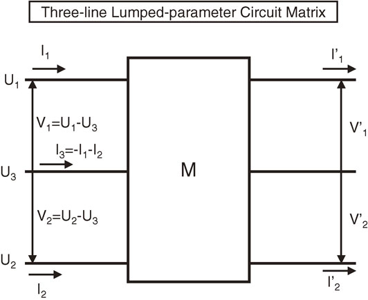
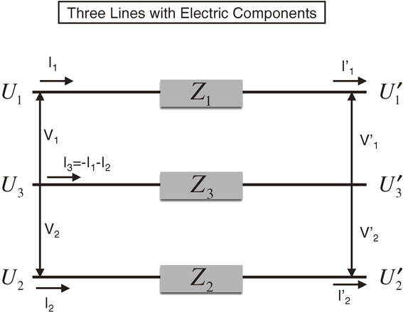
We follow the discussion made in a published paper by Sato and Toki.3) We first describe a three-line circuit as a simple lumped-parameter circuit. We show in Fig. 4 the three-line lumped-parameter circuit matrix $M$, where the three lines are numbered from the above as lines 1, 3 and 2, anticipating that the third line will be used as the ground line (central line of symmetric arrangement). Because we impose that the total current is zero, $I_{3} = - I_{1} - I_{2}$. The associated voltages are usually measured from the third line as $V_{1} = U_{1} - U_{3}$ and $V_{2} = U_{2} - U_{3}$.4) The performance of the electric component is given by the matrix $M$, which relates the initial and final currents and voltages:
| \begin{equation}
\left(
\begin{array}{c}
V_{1}\\
I_{1}\\
V_{2}\\
I_{2}
\end{array}
\right) = \left(
\begin{array}{cccc}
a_{11} & a_{12} & a_{13} & a_{14}\\
a_{21} & a_{22} & a_{23} & a_{24}\\
a_{31} & a_{32} & a_{33} & a_{34}\\
a_{41} & a_{42} & a_{43} & a_{44}
\end{array}
\right)\left(
\begin{array}{c}
V'_{1}\\
I'_{1}\\
V'_{2}\\
I'_{2}
\end{array}
\right).
\end{equation}
| [1] |
Matrix
M is usually a complicated
$4 \times 4$ matrix with some coefficients,
$a_{ij}$, being finite.
It is very important now to introduce a concept of normal and common modes for discussing noises.3) We consider lines 1 and 2 to be the main lines, and line 3 as the ground line. These main lines (1 and 2) are designed by engineers for good performance, while no attention is paid to line 3. However, as noticed in the noise pulse of TARN2, we should design also the third line to reduce noise. We have to find a condition to minimize the effect of the third line on the main lines. For this purpose, we define here first the normal-mode current and voltage:
| \begin{equation}
I_{n} = \frac{1}{2}(I_{1} - I_{2}),
\end{equation}
| [2] |
| \begin{equation}
V_{n} = U_{1} - U_{2} = V_{1} - V_{2}.
\end{equation}
| [3] |
These quantities are those used for the two-line circuit, where the total current of a two-line system is zero, or
$I_{1} + I_{2} = 0$. If this is the case, the normal-mode current becomes
$I_{n} = I_{1} = - I_{2}$, and
$V_{n}$ is the potential difference between lines 1 and 2. Hence, the normal mode is the standard mode used in any two-line circuit. It is important to keep in mind that the normal mode is the mode that we consider for the design of an electric circuit. What is special in three-line circuit is the presence of the so-called common mode. The common-mode current and voltage are defined as
| \begin{equation}
I_{c} = \frac{1}{2}(I_{1} + I_{2} - I_{3}),
\end{equation}
| [4] |
| \begin{equation}
V_{c} = \frac{1}{2}(U_{1} + U_{2}) - U_{3}.
\end{equation}
| [5] |
These quantities are never considered for the treatment of a two-line circuit. With the condition of the total current being zero for the three lines,
$I_{1} + I_{2} + I_{3} = 0$, the common-mode current
[4] becomes
$I_{c} = I_{1} + I_{2}$. Usually the summed current is assumed to be zero in the two-line circuit. Hence, the common mode is a mode associated with the third line, which is considered to be the ground line. Because of the definition of the normal and common modes, these quantities are often called the differential mode (normal mode) and the summed mode (common mode). With the normal and common modes so defined, we can express the performance of an electric element by using another matrix,
$M_{nc}$:
| \begin{equation}
\left(
\begin{array}{c}
V_{n}\\
I_{n}\\
V_{c}\\
I_{c}
\end{array}
\right) = \left(
\begin{array}{cccc}
b_{11} & b_{12} & b_{13} & b_{14}\\
b_{21} & b_{22} & b_{23} & b_{24}\\
b_{31} & b_{32} & b_{33} & b_{34}\\
b_{41} & b_{42} & b_{43} & b_{44}
\end{array}
\right)\left(
\begin{array}{c}
V'_{n}\\
I'_{n}\\
V'_{c}\\
I'_{c}
\end{array}
\right).
\end{equation}
| [6] |
This matrix
$M_{nc}$ is related to the original matrix
M.
We now calculate a simple three-line circuit with impedances $Z_{1}$, $Z_{2}$ and $Z_{3}$, as shown in Fig. 5 in order to understand the meaning of the normal and common modes. In this case, $V_{1} = V'_{1} + (Z_{1} + Z_{3})I'_{1} + Z_{3}I'_{2}$ and $V_{2} = V'_{2} + (Z_{2} + Z_{3})I'_{2} + Z_{3}I'_{1}$, where $I_{1} = I'_{1}$ and $I_{2} = I'_{2}$. Hence, in the original $4 \times 4$ matrix $M$, many matrix elements are zero, and mode 1 and mode 2 couple with each other. In terms of the new variables, these relations are written as $V_{n} = V'_{n} + (Z_{1} + Z_{2})I'_{n} + \tfrac{1}{2}(Z_{1} - Z_{2})I'_{c}$ and $V_{c} = V'_{c} + (\tfrac{1}{4}(Z_{1} + Z_{2}) + Z_{3})I'_{c} + \tfrac{1}{2}(Z_{1} - Z_{2})I'_{n}$. Hence, the matrix $M_{nc}$ is:
| \begin{equation}
{M_{nc} = \left(
\begin{array}{cccc}
1 & Z_{1} + Z_{2} & 0 & \tfrac{1}{2}(Z_{1} - Z_{2})\\
0 & 1 & 0 & 0\\
0 & \tfrac{1}{2}(Z_{1} - Z_{2}) & 1 & \tfrac{1}{4}(Z_{1} + Z_{2}) + Z_{3}\\
0 & 0 & 0 & 1
\end{array}
\right).}
\end{equation}
| [7] |
This matrix indicates that, generally, the normal mode couples with the common mode. A very interesting observation is, however, that the non-diagonal matrix elements become zero when the two impedances are equal,
$Z_{1} = Z_{2}$. Hence, if we keep the symmetry around the third line by the arrangement of electric elements, we can decouple the normal mode from the common mode. Usually, some filtering device and impedance matching are arranged for the normal mode. However, if the circuit is asymmetric around the third line, uncontrolled noises in the common mode without any noise filter and impedance matching mix into the normal mode, and the performance becomes unexpectedly worse. This was the case of TARN2, where a huge noise in the common mode disturbed the operation of the accelerator. Similarly, in conventional two-line circuits consisting of asymmetrically arranged lumped circuit elements, the noise in the common mode appears to be unavoidable.
In a paper by Sato and Toki,3) the HIMAC system with the power supply, noise filter and magnet complex is analyzed using the normal-common mode matrix, $M_{nc}$, of Eq. [6]. As far as a lumped-parameter three-line circuit is concerned, we are able to show that a symmetric three-line circuit with twin power supplies and filtering elements should eliminate high-frequency electromagnetic noise by a special arrangement of the electric lines. Here, it is essential to connect the third line (ground line) to the middle point of the twin power supplies. This is very important to make the symmetrically arranged filtering circuit to act efficiently by reducing any high-frequency noise in the common mode in addition to that in the normal mode.3)
IV. New three-conductor transmission-line theory with coefficients of the potential
The electromagnetic noise is usually a high-frequency wave, and we have to consider that all of the lines have electromagnetic functions for any real description of noise. Hence, we consider the performance of three-conductor transmission lines, which is a distributed-parameter circuit. We here follow a paper of Toki and Sato.6)
We start with a conventional multi-conductor transmission-line (MTL) theory, written systematically for an example in a book of Paul.4) We note here in advance that the conventional MTL theory will be replaced by a new circuit theory. Although the MTL theory treats a distributed-parameter circuit, its variables of the three-conductor transmission lines are defined similarly to those in the previous section: $V_{1},I_{1}$, and $V_{2},I_{2}$ in Fig. 5. We treat the simplest case, where all of the lines are lossless. These quantities are now functions of distance from one terminal of the lines, the coordinate of which is written as the z-axis. These quantities are also functions of time t. The voltages and currents follow the MTL differential equations4):
| \begin{equation}
\frac{\partial V_{i}(z,t)}{\partial z} = -\sum_{j} \mathcal{L}_{ij}\frac{\partial I_{j}(z,t)}{\partial t},
\end{equation}
| [8] |
| \begin{equation}
\frac{\partial I_{i}(z,t)}{\partial z} = -\sum_{j} \mathcal{C}_{ij}\frac{\partial V_{j}(z,t)}{\partial t}.
\end{equation}
| [9] |
Here, suffices
i,
j are 1 and 2 for three-conductor transmission lines. The condition that the total current is zero has been imposed:
$I_{1} + I_{2} + I_{3} = 0$. The quantities
$\mathcal{L}_{ij}$ are
the coefficients of the inductance and the quantities
$\mathcal{C}_{ij}$ are
the coefficients of the capacitance. These quantities are calculated for various configurations of MTL systems in the book of Paul.
4) The MTL equations are written using a displacement current going through a capacitance and a true current following Kirchhoff’s current law.
9) As discussed in the previous section, it is important to introduce the normal-mode quantities
$V_{n}$ and
$I_{n}$ to define the standard mode. We should also introduce the common-mode quantities
$V_{c}$ and
$I_{c}$. When we introduce the normal and common modes to the conventional MTL equations, however, we immediately encounter a difficulty to express the MTL equations in terms of the normal- and common-mode quantities. We will soon explain why
$C_{ij}$ is not suited for mathematical manipulations.
To this end, we first take an idea to treat all of the three lines on equal footing, and use all 6 variables, $U_{i},I_{i}$ with $i = 1,2,3$ in Fig. 5, where $U_{i}$ is a potential measured from an infinite distance. We can then rewrite the above MTL equations as
| \begin{equation}
\frac{\partial U_{i}(z,t)}{\partial z} = -\sum_{j = 1}^{3}L_{ij}\frac{\partial I_{j}(z,t)}{\partial t},
\end{equation}
| [10] |
| \begin{equation}
\frac{\partial I_{i}(z,t)}{\partial z} = -\sum_{j = 1}^{3}C_{ij}\frac{\partial U_{j}(z,t)}{\partial t}.
\end{equation}
| [11] |
In the book of Paul,
4) these coefficients,
$L_{ij}$ and
$C_{ij}$, are called generalized coefficients. These coefficients in
Eqs. [10] and
[11] are related to the corresponding coefficients
$\mathcal{L}_{ij}$ and
$\mathcal{C}_{ij}$, written in
Eqs. [8] and
[9]. We mention here that the relations of
$L_{ij}$ and
$\mathcal{L}_{ij}$ are simple, while the relations of
$C_{ij}$ and
$\mathcal{C}_{ij}$ are complicated.
4) This is caused by the fact that the constraint condition that the total current be zero provides complicated expressions for
$C$. Anticipating the discussion of radiation from an electric circuit in the next section, we define the
antenna mode in addition to the normal and common modes:
| \begin{equation}
V_{n} = U_{1} - U_{2},
\end{equation}
| [12] |
| \begin{equation}
V_{c} = \frac{1}{2}(U_{1} + U_{2}) - U_{3},
\end{equation}
| [13] |
| \begin{equation}
U_{a} = \frac{1}{2}\left(\frac{1}{2}(U_{1} + U_{2}) + U_{3} \right),
\end{equation}
| [14] |
for the normal-mode voltage,
$V_{n}$, and the common-mode voltage,
$V_{c}$, where these quantities are defined as differences of potentials. On the other hand, the antenna-mode potential,
$U_{a}$, is not a voltage, but a potential, itself, measured from an infinite distance. An electromagnetic wave is emitted and absorbed through the antenna mode. Similarly, we define all of the currents as
| \begin{equation}
I_{n} = \frac{1}{2}(I_{1} - I_{2}),
\end{equation}
| [15] |
| \begin{equation}
I_{c} = \frac{1}{2}(I_{1} + I_{2} - I_{3}),
\end{equation}
| [16] |
| \begin{equation}
I_{a} = I_{1} + I_{2} + I_{3},
\end{equation}
| [17] |
for the normal-mode current,
$I_{n}$, the common-mode current,
$I_{c}$, and the antenna-mode current,
$I_{a}$. It is an interesting fact that Kirchhoff was the first author to introduce a potential in a single wire theory in 1857.
10) This consideration of propagation of electromagnetic waves in a single wire was abandoned by Heaviside, who introduced two wires for the propagation of electromagnetic waves through an electric circuit in 1881.
9) In this section, we first take the condition without the antenna mode, namely
$I_{a} = 0$, and the total current is zero
$I_{t} = I_{1} + I_{2} + I_{3} = 0$. Then, in the next section, we remove this condition and discuss the most general circuit theory using the Maxwell equations.
7)
In the effort of writing the conventional MTL equations in terms of the normal and common modes, we encounter a difficulty to express the differential equations in a compact way. This difficulty originates from the treatment of the coefficients of capacitance, $C_{ij}$. As discussed above, it is difficult to treat the constraint condition that the total current is zero in the expression with $C_{ij}$. Hence, we rearrange the differential equations involving the $C$ terms by expressing the potentials in terms of the currents as
| \begin{equation}
\frac{\partial U_{i}(z,t)}{\partial t} = - \sum_{j = 1}^{3} P_{ij}\frac{\partial I_{j}(z,t)}{\partial z}.
\end{equation}
| [18] |
Hence, the coefficients
$P_{ij}$ in
Eq. [18] satisfy the inverse matrix relation:
| \begin{equation}
P_{ij} = (C^{-1})_{ij}.
\end{equation}
| [19] |
The quantities
$P_{ij}$ are called
coefficients of potential.
4),5) This naming of the quantities
$P_{ij}$ were made by Maxwell, while considering that potentials are written in terms of charges using these coefficients.
5) This procedure of using
$P_{ij}$ instead of
$C_{ij}$ is not merely mathematical manipulations. We arrive at the differential equations
[18] directly using Coulomb’s law and the continuity equation relating the charge and the current in a wire. Hence, we do not use the concept of the displacement current and Kirchhoff’s current law in the present new MTL theory. Using
$P$ we are able to express the MTL equations simply in terms of the normal- and common-mode quantities.
We first show the differential equations for the normal and common modes involving $L$:
| \begin{equation}
\frac{\partial V_{n}(z,t)}{\partial z} = -L_{n}\frac{\partial I_{n}(z,t)}{\partial t} - L_{nc}\frac{\partial I_{c}(z,t)}{\partial t},
\end{equation}
| [20] |
| \begin{equation}
\frac{\partial V_{c}(z,t)}{\partial z} = -L_{nc}\frac{\partial I_{n}(z,t)}{\partial t} - L_{c}\frac{\partial I_{c}(z,t)}{\partial t}.
\end{equation}
| [21] |
These coefficients are written in terms of coefficients of inductance, defined in
Eq. [10], for each line:
| \begin{equation}
L_{n} = L_{11} + L_{22} - 2L_{12},
\end{equation}
| [22] |
| \begin{equation}
L_{c} = \frac{1}{4}(L_{11} + L_{22} + 2L_{12}) + L_{33} - L_{13} - L_{23},
\end{equation}
| [23] |
| \begin{equation}
L_{nc} = L_{cn} = \frac{1}{2}(L_{11} - L_{22}) - L_{13} + L_{23}.
\end{equation}
| [24] |
We note here that all of the coefficients in the equations for the normal and common modes are written in terms of the summation and subtraction of the original coefficients,
$L_{ij}$. These quantities are in general non-vanishing, and the normal and common modes couple with each other. We can make the same manipulations to write differential equations for the normal and common modes involving the
$P$ terms:
| \begin{equation}
\frac{\partial V_{n}(z,t)}{\partial t} = -P_{n}\frac{\partial I_{n}(z,t)}{\partial z} - P_{nc}\frac{\partial I_{c}(z,t)}{\partial t},
\end{equation}
| [25] |
| \begin{equation}
\frac{\partial V_{c}(z,t)}{\partial t} = -P_{nc}\frac{\partial I_{n}(z,t)}{\partial z} - P_{c}\frac{\partial I_{c}(z,t)}{\partial z}.
\end{equation}
| [26] |
These coefficients
$P$ are written in terms of the coefficients for each line defined in
Eq. [18]:
| \begin{equation}
P_{n} = P_{11} + P_{22} - 2P_{12},
\end{equation}
| [27] |
| \begin{equation}
P_{c} = \frac{1}{4}(P_{11} + P_{22} + 2P_{12}) + P_{33} - P_{13} - P_{23},
\end{equation}
| [28] |
| \begin{equation}
P_{nc} = P_{cn} = \frac{1}{2}(P_{11} - P_{22}) - P_{13} + P_{23}.
\end{equation}
| [29] |
We note here again that all of the coefficients in the equations for both the normal and common modes are written in terms of the summation and subtraction of the original coefficients,
$P_{ij}$. If these are the coefficients of capacitance, the coefficients involve divisions and multiplications of the original coefficients,
$C_{ij}$, and the expressions are highly complicated. Again, in general the normal and common modes couple with each other. We shall call these differential equations [
20,
21] and [
25,
26] as Toki-Sato MTL (TS-MTL) equations.
We now consider the condition that the coupling terms of the normal and common modes are zero, $L_{nc} = P_{nc} = 0$. Then, the differential equations for the normal mode are:
| \begin{equation}
\frac{\partial V_{n}(z,t)}{\partial z} = -L_{n}\frac{\partial I_{n}(z,t)}{\partial t},
\end{equation}
| [30] |
| \begin{equation}
\frac{\partial V_{n}(z,t)}{\partial t} = -P_{n}\frac{\partial I_{n}(z,t)}{\partial z}.
\end{equation}
| [31] |
These equations for the normal mode are decoupled from the differential equations for the common mode:
| \begin{equation}
\frac{\partial V_{c}(z,t)}{\partial z} = -L_{c}\frac{\partial I_{c}(z,t)}{\partial t},
\end{equation}
| [32] |
| \begin{equation}
\frac{\partial V_{c}(z,t)}{\partial t} = -P_{c}\frac{\partial I_{c}(z,t)}{\partial z}.
\end{equation}
| [33] |
We can verify that these equations for the normal mode completely agree with the two-conductor transmission-line equations, including the expressions of all the coefficients.
4),6) The equations for the common mode are completely new.
6)
In order to understand the condition that the normal mode decouples from the common mode ($L_{nc} = P_{nc} = 0$), we have to express all of the coefficients explicitly. For this purpose, we take the Neumann relation for the coefficients of inductance for thin wires.4),6),11) Here, the Neumann relation is obtained by calculating the vector potential while using Ampere’s law at the surface of the i-th wire caused by the current through the j-th wire11):
| \begin{equation}
L_{ij} = \frac{\mu}{2\pi}\left(\ln\frac{2l}{a_{ij}} - 1 \right).
\end{equation}
| [34] |
Above,
$l$ denotes the length of the wires, and
$a_{ij}$ is the radius of the
i-th wire
$(i = j)$ and the distance between the wires
i and
j for
$i \ne j$. We can see that these coefficients are symmetric,
$L_{ij} = L_{ji}$. We may also take into account the skin effect in these size and distance parameters.
11) It is very important to note that we are able to use the same Neumann relation for the coefficients of the potential for thin wires. Here, the Neumann relation is obtained by calculating the scalar potential using Coulomb’s law at the surface of the
i-th wire caused by the charge in the
j-th wire.
6) Thus, we find similar expressions for
$P_{ij}$:
| \begin{equation}
P_{ij} = \frac{1}{2\pi \varepsilon}\left(\ln\frac{2l}{a_{ij}} - 1 \right).
\end{equation}
| [35] |
In the simplest case, these coefficients are the same, except for
$\mu $ and
$\varepsilon $. As in the case of
$L$, discussed above,
$P$ has the same simple geometrical meaning. In actual cases, we should consider dielectric materials around wires and any proximity effects.
4) Hence, we keep using
L and
P in this paper instead of combining them in terms of characteristic impedance,
Z.
4)
We thus discuss the condition $L_{nc} = P_{nc} = 0$. The explicit expression
| \begin{equation}
L_{nc} = \frac{1}{2}(L_{11} - L_{22}) - L_{13} + L_{23} = \frac{\mu}{4\pi}\ln\frac{a_{22}a_{13}^{2}}{a_{11}a_{23}^{2}}
\end{equation}
| [36] |
indicates that the shapes of wires 1 and 2 have to be the same (
$a_{11} = a_{22}$), and that the distances of these wires to wire 3 (
$a_{13} = a_{23}$) must be the same. This condition means that the decoupling condition is to place the third line in the middle of the two equivalent main lines 1 and 2. We can impose the same conclusion for the coefficients of the potential. It is now very interesting to write the coefficients of the normal mode as
| \begin{equation}
L_{n} = L_{11} + L_{22} - 2L_{12} = \frac{\mu}{2\pi}\ln\frac{a_{12}^{2}}{a_{11}a_{22}},
\end{equation}
| [37] |
| \begin{equation}
P_{n} = P_{11} + P_{22} - 2P_{12} = \frac{1}{2\pi \varepsilon}\ln\frac{a_{12}^{2}}{a_{11}a_{22}}.
\end{equation}
| [38] |
These expressions are precisely those of a two-conductor transmission-line circuit.
4) The normal mode is considered by engineers for their electric circuits. In actual cases, we may use dielectric materials around the wires, and consider the effects of proximity.
4) However these complications do not change the statement that the third line (ground line) has to be arranged in the center of the two main lines in order to decouple the normal mode from the common mode. The proximity effect acts symmetrically on the main lines if the third line is placed in the middle of the two main lines. Coefficients
P and
L change symmetrically in this case.
4) This is the only way to minimize the effects of the common mode, which goes through the third (ground) line. We want to repeat here that introducing the coefficients of the potential is essential to find simple expressions for the decoupling condition for both the normal and common modes. We show in the next section that the concept of using
P instead of
C makes it possible to derive a new circuit theory that includes radiation from Maxwell’s equations.
V. New circuit theory with antenna mode
We experience electromagnetic noise as a form of radiation noise like that from transmission lines when conduction noise propagates through transmission lines in an electric circuit. We also know that a one-line antenna is able to carry electric power through the antenna line, and produces radiation from it. It is important to note that antenna theory considers the retardation effect of the electromagnetic potentials. On the other hand, MTL theory seems to use only a part of electromagnetism for calculating the coefficients L, C and P.4),6) This is caused by the condition that the total current is zero. We now remove this condition, and discuss the radiation process from a transmission-line system. In addition, it is important to understand the MTL equations from Maxwell’s equations with the help of the definition of the antenna-mode potential, $U_{a}$, of Eq. [14]. Here, we follow a paper by Toki and Sato.7)
A. Retarded potentials for radiation.
We would like to start from Maxwell’s equations, and write the scalar potential, U, and the vector potential, $\vec{A}$, in the Lorenz gauge:
| \begin{equation}
\left(\vec{\nabla}^{2} - \frac{\partial^{2}}{c^{2}\partial t^{2}} \right)U(\vec{x},t) = \frac{1}{\varepsilon} q(\vec{x},t),
\end{equation}
| [39] |
| \begin{equation}
\left(\vec{\nabla}^{2} - \frac{\partial^{2}}{c^{2}\partial t^{2}} \right)\vec{A}(\vec{x},t) = \mu\vec{i}(\vec{x},t).
\end{equation}
| [40] |
Here,
$\vec{\nabla }$ is the spatial differentiation vector,
$\vec{\nabla } = (\tfrac{\partial }{\partial x},\tfrac{\partial }{\partial y},\tfrac{\partial }{\partial z})$. Due to the presence of the time derivative terms, these expressions are Lorentz invariant. From the scalar and vector potentials due to the charge
q and current
$\vec{i}$, we obtain the retarded potentials
12):
| \begin{equation}
U(\vec{x},t) = \frac{1}{4\pi \varepsilon}\int d\vec{x}'\frac{q(\vec{x},t - |\vec{x} - \vec{x}'|/c)}{|\vec{x} - \vec{x}'|},
\end{equation}
| [41] |
| \begin{equation}
\vec{A}(\vec{x},t) = \frac{\mu}{4\pi}\int d\vec{x}'\frac{\vec{i}(\vec{x},t - |\vec{x} - \vec{x}'|/c)}{|\vec{x} - \vec{x}'|}.
\end{equation}
| [42] |
These retarded potentials satisfy the above differential equations for the scalar and vector potentials [
39,
40]. When the charge
q and the current
$\vec{i}$ change with time, electromagnetic radiation takes place.
12) We shall derive circuit theory using the retarded potentials [
41,
42], including radiation.
B. One-conductor transmission-line system: antenna circuit.
We would like to understand the method used to arrive at a circuit theory with radiation by considering a one-conductor transmission-line system. The new circuit theory treats the antenna-mode potential, $U_{a}$, in Eq. [14], which is related to the current, $I_{a}$, the total current. In the one-line case, the total current corresponds to the current in one line. In this case, the charge and current exist only in a wire of length l with a small radius, a. We introduce the area-integrated charge, $Q(z,t) = \int d xdyq(\vec{x},t)$, and the area-integrated current, $I(z,t) = \int d xdyi_{x}(\vec{x},t)$. In this integration, we may take into account the skin effect.11) The direction of the current is also averaged out, and the net current direction is assumed to have only the z-direction, the suffix of which is dropped for the integrated current, $I(z,t)$. Here, we can take into account the skin effect, and possibly the dielectric material effect, and write the retarded potentials at the surface of the conductor7):
| \begin{equation}
{U(z,t) = \frac{1}{4\pi \varepsilon}\int_{0}^{l}\,dz'\frac{Q(z',t - \sqrt{(z - z'){}^{2} + d^{2}}/c)}{\sqrt{(z - z'){}^{2} + d^{2}}},}
\end{equation}
| [43] |
| \begin{equation}
{A(z,t) = \frac{\mu}{4\pi}\int_{0}^{l}\,dz'\frac{I(z',t - \sqrt{(z - z'){}^{2} + d^{2}}/c)}{\sqrt{(z - z'){}^{2} + d^{2}}},}
\end{equation}
| [44] |
where
d is related to radius
a by taking into account the skin effect, and possibly the dielectric material effect.
4),11) We suppress the direction of the vector potential, which is parallel to the
z-direction of the current. We calculate the potentials at the surface of the wire,
$r = \sqrt{x^{2} + y^{2}} = a$, which is related to the effective radius,
d. These potentials must influence the current and the charge in the wire. If we know the potentials at the surface of the wire, we can calculate the electric field on the wire surface, which influences the current in the wire by Ohm’s law,
$E_{z}(z) = RI(z)$, where
R is the resistance. We can write this relation in terms of the scalar
[43] and vector potentials
[44]:
| \begin{equation}
-\frac{\partial U(z,t)}{\partial z} - \frac{\partial A(z,t)}{\partial t} = RI(z,t).
\end{equation}
| [45] |
We have in addition the equation of continuity,
| \begin{equation}
\frac{\partial Q(z,t)}{\partial t} + \frac{\partial I(z,t)}{\partial z} = 0.
\end{equation}
| [46] |
We note that this continuity equation holds for both the charge and current in a wire, and does not include the displacement current, as described in the previous section. These four equations (
Eqs. [43],
[44],
[45] and
[46]) provide a set of coupled differential equations for the scalar and vector potentials at the wire surface as well as the charge and current in the wire. With some initial and boundary conditions in the one-line system, we are able to provide the performance of the wire for the transmission of electric signals.
To proceed, we introduce a fixed frequency, $\omega $, for the scalar potential written as $U(z,t) = U(z)e^{j\omega t}$ and for other quantities written similarly. We can then write the scalar potential [43] as
| \begin{equation}
U(z) = \frac{1}{4\pi \varepsilon}\int_{0}^{l}\,dz'\frac{Q(z')e^{-j\omega \sqrt{(z - z')^{2} + d^{2}}/c}}{\sqrt{(z - z'){}^{2} + d^{2}}}.
\end{equation}
| [47] |
Here, the exponential function has both real and imaginary components:
| \begin{align}
e^{-j\frac{\omega}{c}\sqrt{(z - z'){}^{2} + d^{2}}} &= \cos\biggl(\frac{\omega}{c}\sqrt{(z - z'){}^{2} + d^{2}} \biggr) \\
&\quad- j\sin\biggl(\frac{\omega}{c}\sqrt{(z - z'){}^{2} + d^{2}} \biggr).
\end{align}
| [48] |
The real part has a singular behavior at
$z' \sim z$, and we may pull out the unknown charge from the integral by setting
$Q(z') = Q(z)$:
| \begin{align}
U^{r}(z) &\sim \frac{1}{4\pi \varepsilon}\int_{0}^{l}\,dz'\frac{\cos\frac{\omega}{c}\sqrt{(z - z'){}^{2} + d^{2}}}{\sqrt{(z - z'){}^{2} + d^{2}}}Q(z)\\
& = P(d,\omega)Q(z).
\end{align}
| [49] |
The coefficient
$P(d,\omega )$ has a similar expression as the Neumann relation
[35]. If we set
$\omega = 0$ in
$P(d,\omega )$, then this coefficient agrees with the one written before using the Neumann relation. This singular integral is the source of the MTL equations written in the differential form
[18]. On the other hand, the imaginary part does not have a singular behavior, and we should keep the charge with the integration variable
$Q(z')$ in the integral:
| \begin{equation}
\tilde{U}(z) = -\frac{j}{4\pi \varepsilon}\int_{0}^{l}\,dz'\frac{Q(z')\sin\frac{\omega}{c}\sqrt{(z - z'){}^{2} + d^{2}}}{\sqrt{(z - z'){}^{2} + d^{2}}}.
\end{equation}
| [50] |
We call this
$\tilde{U}$ as a radiation term related to the charge. Hence, we are able to write the scalar potential as
| \begin{equation}
U(z) = P(d,\omega)Q(z) + \tilde{U}(z).
\end{equation}
| [51] |
Similarly, we can perform the same procedure for the vector potential,
| \begin{equation}
A(z) = L(d,\omega)I(z) + \tilde{A}(z).
\end{equation}
| [52] |
The expression for
$L(d,\omega )$ is again similar to the Neumann relation
[35]. We call
$\tilde{A}$ a radiation term related to the current.
Using these expressions for the scalar potential [51] and vector potential [52] together with Ohm’s law [45] and the equation of continuity [46], we arrive at the following new equations:
| \begin{equation}
\frac{\partial U(z,t)}{\partial t} = -P(d,\omega)\frac{\partial I(z,t)}{\partial z} + \frac{\partial \tilde{U}(z,t)}{\partial t},
\end{equation}
| [53] |
| \begin{align}
\frac{\partial U(z,t)}{\partial z} &= -L(d,\omega)\frac{\partial I(z,t)}{\partial t} - \frac{\partial \tilde{A}(z,t)}{\partial t} \\
&\quad- RI(z,t).
\end{align}
| [54] |
Here, the time-dependent quantity
$U(z,t)$ is written as
$U(z,t) = U(z)e^{j\omega t}$, and other quantities are written similarly. If we drop the radiation terms,
$\tilde{U}(z,t)$ and
$\tilde{A}(z,t)$, and arrange the above equations slightly, these equations correspond to the electron-wave transport equation that Kirchhoff derived almost 150 years ago.
10) It is amazing to see that the coefficients of the potential and the inductance were written by Kirchhoff as being proportional to
$\ln \tfrac{l}{a}$ with
l being the length of the line and
a the radius of the line, which agrees the Neumann relation for
L [34] and
P [35]. We also note that this is the first time to derive the transmission equation from Maxwell’s equations including the conduction and radiation of electromagnetic waves for a one-line system, simultaneously. This was possible for us because we had written the MTL equations in terms of the coefficients of the potential.
6) If we drop the tilde terms in the above equations
[53,
54], we arrive at the MTL equations,
[10] and
[18].
We call the above integro-differential equations [53, 54] a new circuit theory for a one-line antenna.7) We are able to verify that the set of equations [53, 54] can give the conduction of an electromagnetic signal through the one-wire circuit and at the same time the radiation from it. The reason why the conduction and radiation occur simultaneously is because the coefficients of potential are vital to definitely determine the potential of one conductor, and thus a duality of the electric and magnetic fields is valid even for one conductor. The antenna mode potential, $U_{a}$, of Eq. [12] is equivalent to U of Eq. [51] for the one-wire case. We can verify that the electromagnetic energy given to the one-wire system is radiated by the antenna process in addition to the loss due to the resistance, R.7)
C. Multi-conductor transmission line theory: new circuit theory.
We can now extend the single-conductor transmission-line theory to a multi-conductor transmission-line theory by extending the differential equations for each line, which are numbered as $i = 1,2 \ldots N$:
| \begin{equation}
\frac{\partial U_{i}(z,t)}{\partial t} = -\sum_{j}^{N}P_{ij}\frac{\partial I_{j}(z,t)}{\partial z} + \frac{\partial \tilde{U}(z,t)}{\partial t},
\end{equation}
| [55] |
| \begin{align}
\frac{\partial U_{i}(z,t)}{\partial z} &= -\sum_{j}^{N}L_{ij}\frac{\partial I_{j}(z,t)}{\partial t} - \frac{\partial \tilde{A}(z,t)}{\partial t} \\
&\quad- R_{i}I_{i}(z,t).
\end{align}
| [56] |
The tilde quantities,
$\tilde{U}$ and
$\tilde{A}$, do not depend on the line number, since we treat the case where all of the lines are placed close to each other as compared to the entire length,
l, of wires. In this case, we have both charge and current in the integral of the tilde potentials as the total charge and total current. These equations provide the conduction and radiation of electromagnetic waves through a MTL system. We here skip all of the details concerning the performance of the coupled equations of the new circuit theory, which is given in a paper of Toki and Sato.
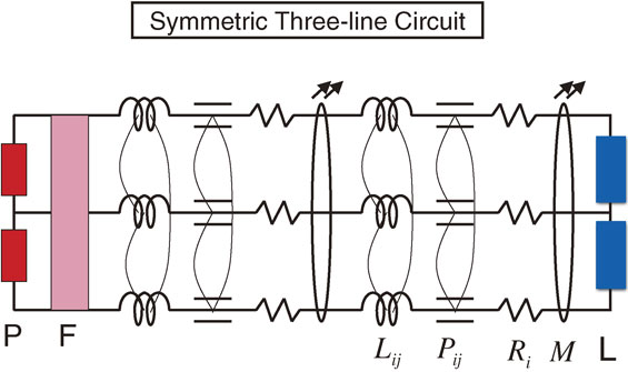
7) Instead, we prefer to consider the figure of a three-line circuit reflecting all of the ingredients of the new circuit theory [
55,
56]. The transmission part of
Fig. 6 is treated by the new circuit theory. The coefficients of the inductance are shown by
$L_{ij}$ using the same symbol as before, but the coefficients of the potential are shown by
$P_{ij}$ using a new symbol, because the coefficients of the capacitance disappear in the new circuit theory. Each line has a resistance indicated by
$R_{i}$, and the antenna function is denoted by
M in the transmission-line part. We also include twin power supplies, denoted as
P, and twin noise filters, denoted as
F on the left side of the transmission lines. Further, we attach a symmetrically arranged electric load, denoted as
L, on the right-hand side of
Fig. 6.
We have introduced the concept of the normal, common and antenna modes, and modified the circuit theory equations for a three-conductor transmission line system. We should use the relations for all of the quantities given in Eqs. [12, 13, 14] and [15, 16, 17]. This manipulation can be done straightforwardly, as worked out in the previous section. We obtain coupled equations of these normal, common and antenna modes.7) The symmetric three-line condition is able to decouple the normal mode from the common and antenna modes. The conditions are completely the same: namely, the main lines 1 and 2 have the same sizes and properties, and the distance of line 1 to line 3 and that of line 2 to line 3 must be the same. These conditions are exactly the same as the case discussed in the new MTL theory with the condition $I_{1} + I_{2} + I_{3} = 0$, as presented in the previous section. We can also show that the common mode always couples with the antenna mode. This finding agrees with our observations that the radiation noise exists whenever we find conduction noise in circuits.
With a new circuit theory, we are now able to propose the best electric circuit, where all of the noises are suppressed for the use of electric devices, as shown in Fig. 6. To start with, an electric circuit has to have three-conductor transmission lines. If a circuit has only two lines, any noise associated with a power supply goes through the two lines and circumstances (ground). Hence, we are not able to control the common-mode noise. Once a circuit has three-lines with the third hard-wired central ground line, we place all of the electric components symmetrically around the third central ground line. The main two lines (upper and lower lines) should have the same sizes and same properties, and at the same time the distances of the two main lines to the third line must be the same. The power supplies should be arranged symmetrically around the middle point of twin power supplies, so that the noises in the normal and common modes produced in the power supplies are confined in the circuit. Then, the symmetrically arranged filtering elements are able to reduce any high-frequency noises in both the normal and common modes. Some noises from the grounding may go through the three-conductor transmission lines, but the normal mode is decoupled from the common mode. When we use some electric elements to perform something, we should also arrange them symmetrically around the third line, and try to use only the normal-mode voltage and current.
VI. Application of the new circuit theory
A. HIMAC power supply, noise filter and magnet system.
The HIMAC power supply, noise filter and magnet complex was built on the basis of a theoretical study of a symmetric three-line (S3L) circuit using the lumped-parameter circuit theory before the present new multi-conductor transmission-line (MTL) theory was constructed. Using the lumped-parameter circuit theory, we can show that the S3L circuit is good to first decouple the normal mode from the common mode, and the symmetric arrangement of filtering elements works very effectively to reduce any noises in both the normal and common modes3); conversely, a non-symmetric circuit is not good for the normal mode being coupled with the common mode, and no filtering elements can work well to reduce the noises.
In the practice of making the S3L circuit for HIMAC, the hard-wired central ground line was introduced to the two main lines, as shown in Fig. 1. The two main lines were connected with magnets symmetrically around the hard-wired central ground line. In addition, the two main lines have the same size, and are equidistant from the central ground line. This symmetric arrangement of three lines was essential for noise reduction, though based on an appropriate guess before the present new circuit theory of MTL was formulated.
The twin power supplies connected in series are arranged symmetrically around the central ground line, which necessarily produce noises in both the normal and common modes due to alternate switching in the twin power supplies. This is particularly the case in recent years due to the use of IGBT and Power MOS-FET devices, which employ chopping methods to modify the forms of the electricity. The filtering elements were also arranged symmetrically around the third central ground line, which were able to reduce any high-frequency noises in both the normal and common modes. The magnet for HIMAC uses only the normal-mode current, where the N-pole uses the upper current (line 1) and the S-pole uses the lower current (line 2), so that the magnetic field at the magnet gap uses only the normal-mode current. The LHC of CERN also uses a S3L power supply and magnet system.
B. Reconfiguration of the J-PARC/MR magnet complex.
The power supply, noise filter and magnet system for the Main-Ring synchrotron of Japan Proton Accelerator Research Complex (J-PARC/MR) was originally a conventional two-line circuit, which disregarded such circumstances as the ground, similar to that of TARN2, as shown in Fig. 2. The power supply used the IGBT method, and the noise level was quite high before the reconfiguration, as shown in the upper figure of Fig. 7. Definitely, noise was created in both the normal and common modes in the power supply. We can imagine that the noise in the normal mode is largely reduced by a noise filter, as in the case of TARN2, while the noise in the common mode is not treated at all in the conventional two-line circuit. In this case, there is an unexpected third line used as the ground, so that the noise in the common mode couples in the normal mode.
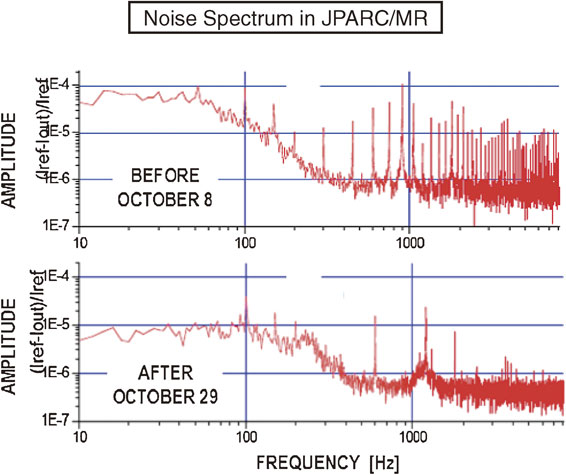
Hence, the J-PARC/MR accelerator group took the idea of HIMAC, and introduced a third hard-wired central ground line, and symmetrized the magnet arrangements around the third line. The accelerator group then used the current in line 1 for the N-poles and the current in line 2 for the S-poles of all the magnets, and thus the magnetic field at the magnet gap was produced only by the normal-mode current, $I_{n} = \tfrac{1}{2}(I_{1} - I_{2})$. Due to the fact that the power supply had no central point, it was only possible to reduce the noise in the normal mode with the noise filter, but not the noise in the common mode, as in the case of HIMAC. The S3L circuit in the magnet part after the power supply and the noise filter components was able to decouple the normal mode from the common mode. They were able to reduce the noise level of the magnetic field by an order of magnitude by using only the normal-mode current, as can be seen in the lower figure of Fig. 7. In the case of dipole magnets, the noise level of $\Delta I/I_{DC}$ was improved by a factor of 20 from $2 \times 10^{ - 3}$ to $1 \times 10^{ - 4}$ at IDC = 1600 A. After the reconfiguration, beam commissioning was successfully achieved. It turned out, as can be seen from Fig. 7, that the origin of the noise in the case of the conventional two-line circuit is the coupling between the normal and common modes.
We have to mention here that the present situation of the J-PARC/MR power supply and magnet system is that the high-frequency noise in the normal mode is somehow controlled due to the noise filter. However, the noise in the common mode is not reduced at all, as compared to the situation before the symmetric arrangement. Hence, the total noise level is not changed around the J-PARC/MR synchrotron unless twin power supplies, and twin noise filters are equipped with the third hard-wired central ground line. It is important to improve the whole system in order to suppress the noise level to below $\Delta I/I_{DC} = 1 \times 10^{ - 6}$. This is the only way to reduce the noise level completely around the synchrotron.
C. B787 battery and power generation.
It was a serious accident that the battery set of Boeing 787 aircraft (B787) was burnt during several scheduled flights. One large difference of the B787 from other Boeing aircraft is the full use of electricity by using powerful generators and rechargeable batteries. The total power generation is on the order of 1 Megawatt. Two battery sets are placed in the front and middle parts of the Boeing aircraft, and the generators are placed in the middle and the back sections. The generated electricity was carried by transmission lines using a conventional two-line circuit. This means that some amount of the generated power was carried in the common mode using the circumstances (third line). It should be stressed that the quantities in the common mode cannot be measured directly by any usual observation method because of an invisible signal in the two-line circuit. In the case of aircraft, the circumstance is not the ground, but its body. It is usually the case that the grounding is attached to the negative side of the battery set. Hence, the voltage difference between the positive battery cap and the aircraft body is large, and occasionally some flash may attack the positive cap of the battery set.
The usual method used to avoid this type of accident is to introduce a tight protection system and strong insulation between the electric devices, such as batteries, and the circumstances. Although this method was used to cure the problem of the B787 concerning the battery, escaping power from the circuit to the circumstances (ground) would attack other electric devices. The escaped power in the common mode could come back to the two-line circuit at any place due to the coupling of the normal and common modes. Instead, we would like to suggest another solution based on the new circuit theory for stable operation of the B787. We have to be aware of the fact that the strong high-frequency noise produced by the AC to DC converter is not at all reduced, and this noise may cause serious problems in such electric devices as computers and control systems. Following the new circuit theory, it is advisable to use the S3L circuit so that no unnecessary electricity escape from any electric device to the circumstance (ground). In this way, we can avoid accidents due to electromagnetic noises.
We also mention that recent hybrid cars use a strong battery set with strong power generators, on the order of 100 Kilowatts. As in the usual method, a conventional electric circuit is used together with the body-earth method, where the negative cap of the battery set is connected directly to the car body. Electromagnetic noise generated by the IGBT method for the conversion and inversion of DC and AC currents moves freely in the car body. This noise may cause serious problems to such electric devices as computers and control systems. It would be advisable to introduce a S3L circuit to control a large amount of electric power in the common mode for such high-power machines as hybrid cars and others.
D. Anticipation of a new paradigm of basic electromagnetism.
The Maxwell equations consist of a set of four partial differential equations for electric and magnetic fields, and form the foundation of basic electromagnetism. In 1861 Maxwell added a displacement current, which is proportional to the derivative of the electric field with respect to time, to the electric current term in Ampere’s law.14) This addition of the displacement current term was the key to understanding and producing the electromagnetic wave, and thus to complete the concept of electromagnetism. As far as the electromagnetic wave equation is concerned, however, the naming of the displacement current is mis-leading, and hence this additional term is often called Maxwell’s correction term.15) On the other hand, the concept of the displacement current was used by Heaviside in 1881 in the theory of transmission lines using a capacitance for a network of infinitesimally small circuit elements with Kirchhoff’s current law.9) It should be noted from the present study of the MTL theory that the displacement current through a capacitance is not necessary despite the fact that Maxwell’s correction term surely exists. Instead, conductor lines have now been related through the electromagnetic fields (scalar and vector potentials), and all of the charges and currents being confined in each line satisfy the continuity equation.
The present study of the MTL theory was motivated in order to understand the mystery of noise production following the success of a new practice of noise reduction using a S3L circuit adopted for the first time in HIMAC. The new circuit theory that includes radiation is based on the retarded potential obtained from Maxwell’s equations, which naturally leads to the coefficients of the potential in the same way as the coefficients of inductance. The coexistence of the electric and magnetic phenomena induces the conduction of electric signals along transmission lines and radiation from the transmission lines. Even in the case of a single conductor, the potential of a conductor at each point in the conductor varies with time to provide a conduction wave along the conductor and a radiation wave from the conductor simultaneously. The new circuit theory of a single conductor possesses the duality of the electric and magnetic fields of Maxwell’s equations. In order to complete circuit theory, we need two more relations between electromagnetic fields, charges and currents. The natural relations come from the continuity equation of the true charge and the conduction current inside a conductor, as well as the boundary condition at the surface of conductor given by Ohm’s law inside the conductor. The principles of the circuit theory mentioned above are completely different from those of the conventional two-conductor transmission-line theory, which is based on the coefficients of the capacitance.
The conventional MTL theory needs at least two conductor lines due to the use of capacitance. Because a displacement current goes through a capacitance between conductors, Kirchhoff’s current law is satisfied using both the displacement current and the true current. The conventional MTL theory uses Kirchhoff’s current law as a lumped-parameter circuit theory for two or more conductors so that electric waves go through a MTL system consisting of more than two conductors. The potential of a single conductor is not determined definitely in the conventional MTL theory. Hence, the radiation phenomenon from a single conductor is treated separately from the conduction wave along the conductor. The principle of the transmission line theory should be deeply related to the basic concept of electromagnetism.
We want to emphasize that the principle of the new circuit theory is largely different from that of the conventional MTL theory, while the fundamental theory of the basic electromagnetism has to be Maxwell’s equations. Instead of the conventional basic electromagnetism, thus, a new paradigm of basic electromagnetism is anticipated from the new circuit theory, which clears up the mystery of noise production without employing the displacement current, namely the current in the capacitances.
VII. Summary
A new practice of noise reduction began with the encounter to the drawing of a chain of magnets for CERN-PS.2) In addition, it was essential to find a large noise in the common mode in the magnet system of TARN2 at INS. The observation of the electromagnetic noise showed that a noise pulse propagated through the ground so that the ground seemed to play the role of a third line of the two-line magnet system, without noticing its presence. A new design of the power supply, noise filter and magnet system for HIMAC based on the CERN-PS drawing was introduced after many years by making a thorough theoretical study of a S3L circuit using the lumped-parameter circuit theory.1),3) With the third hard-wired central ground line, the complete power supply, noise filter and magnet system was designed to have a S3L circuit that consisted of twin power supplies, twin noise filters and a chain of magnet system. Its operation was very stable and the noise level was on the order of $\Delta I/I_{DC} \sim 10^{ - 6}$.
The new circuit theory was motivated by the success of a new practice of the S3L circuit for HIMAC. A very important concept for noise reduction is the use of the normal and common modes, through which electromagnetic waves propagate along a three-line circuit. It was then realized that the normal mode is completely decoupled from the common mode by arranging the electric elements around the third central ground line using the lumped-parameter circuit theory.3) We began by pursuing a challenge concerning a real three-line circuit theory in order to treat high-frequency noises.6)
The first trial was to introduce the normal and common modes to the MTL theory. We immediately found that the introduction of the normal and common modes was complicated due to the fact that the use of the coefficients of capacitance, C, forced us to perform inversions of equations in several calculation steps. This complication of manipulation with C is caused by the use of the constraint equation of the total current being zero. Hence, we expressed the potentials in terms of the currents for the conventional MTL equations, including the coefficients of the capacitance, C. The coefficients appearing in these equations are P. This was our starting point for constructing a new circuit theory to use the coefficients of the potential P, which are an inverse matrix of the coefficients of the capacitance; $P_{ij} = (C^{ - 1})_{ij}$. This introduction of the coefficients of the potential instead of the coefficients of the capacitance is not merely a mathematical convenience. The resulting differential equations are now obtained by using Coulomb’s law and the continuity equation. Hence, the dynamics of two conductor lines are controlled by the electromagnetic fields, while the charges and currents are confined in each conductor line. It was then easy to introduce the normal and common modes to the modified MTL equations. Since the MTL equations with the normal and common modes have simple forms, we were able to identify the conditions of decoupling of the normal mode from the common mode. We can show that the S3L circuit satisfies the decoupling conditions. The two main lines should have the same sizes, and the qualities and distances of the two main lines to the third line must be the same.
We studied a new circuit theory of the MTL system starting from Maxwell’s equations. Hence, our starting point was the use of the retarded scalar and vector potentials, which are able to provide electromagnetic radiation from time-dependent electric sources. The retarded potentials have both the real and imaginary parts, when expressed for AC with a fixed frequency. The real part provides the L and P terms of the MTL equations, which are responsible for the conduction of electric signals in both normal and common as well as antenna modes. On the other hand, the imaginary part provides a term having the same phase as the resistance term, and is responsible for the radiation of electric waves from an electric circuit through the antenna mode. We could show that the imaginary part corresponds to the radiation from a MTL system, and that the radiation energy agrees with antenna theory.7) We now have a new circuit theory that includes radiation from transmission lines in addition to conduction of electromagnetic waves along transmission lines in a MTL system. With the new circuit theory, we are able to display an ideal electric circuit system. It is important to use a S3L circuit in order to decouple the normal mode from both the common and antenna modes, and then to reduce any high-frequency noise by introducing filtering devices symmetrically around the third ground line.
We now sincerely hope that our new circuit theory of a MTL system resulting from the new practice is able to reduce electromagnetic noise from the circumstance (ground). In the present technology, the IGBT and Power MOS-FET devices produce high-frequency noises. It is important for every user of electricity to use the S3L circuit to completely reduce the electromagnetic noise in their electric circuits. If the powers of electric machines are large, the noise powers in the corresponding common mode will become unexpectedly large. The S3L circuit is a unique method to control electric noises, and hence the noise powers.
Profile

Hiroshi Toki was born in 1946, and started his research career in 1971 with studies on nuclear structure in Osaka University. After obtaining his PhD in Physics in 1974, he went to Juelich Research Institute (KFA Juelich) in West Germany, and there studied theoretically the high-spin states of nuclei. He enlarged his research interest to include hadron physics, and subsequently pioneered quark-nuclear physics after moving to Regensburg University in 1977. His interest was the pion- and quark-structures of the nucleus and nuclear matter, and his theoretical predictions urged many experiments worldwide. He was invited by Michigan State University in 1980 to be an Assistant Professor, where he taught many students, and deepened his study of the role of pions on nuclear structure. He returned to Tokyo Metropolitan University as an Associate Professor in 1983, and started to supervise many students for doctor theses in the field of quark-, pion- and relativistic-nuclear physics. He made important contributions to nuclear physics, such as predictions of deeply bound pionic atoms, the relativistic equation of state of nuclear matter, as well as dual Ginzburg-Landau theory on quark confinement. He was awarded the Japan Physical Society (JPS) Prize of Outstanding Paper and the Humboldt Research Prize for his contributions in the field of quark- and pion-nuclear physics. He became a Professor at Research Center for Nuclear Physics (RCNP) of Osaka University in 1994, and was appointed as the Director of RCNP in 2001 for 6 years. He started to work on the electromagnetic noise and multiconductor transmission-line theory with his collaborator, Prof. K. Sato, in 2005, and contributed largely to the completion of J-PARC/MR accelerator. This work was awarded the JPS Prize of Outstanding Paper in 2011. He then worked several years for the Japan Physical Society and Osaka University as an executive committee member.
Profile
Kenji Sato was born in Osaka, Japan, in 1942. He received a BS degree from the Department of Physics, Osaka University, in 1965. While attending graduate school at Osaka University from 1965 to 1971, he received a MS degree in 1967, and later received a Ph.D. degree in 1975. His professional career as an accelerator physicist started in 1971 at the Institute for Nuclear Study (INS), University of Tokyo, as a member of the construction group that developed the sector focusing (SF) cyclotron. In 1982, he joined Gesellschaft fur Schwerionen Forschung (GSI) in West Germany to develop a heavy-ion synchrotron (SIS). After his return to INS in 1983, he studied and successfully developed a broadband rf accelerating cavity for a cooler-synchrotron, TARN2. In 1988, he joined the National Institute of Radiological Sciences (NIRS) and was responsible for constructing the twin synchrotrons of the Heavy Ion Medical Accelerator in Chiba (HIMAC). Based on his design of a symmetric three-line circuit, he succeeded to develop a very low-noise system that consisted of a power supply, filter, and magnet chain. Soon after the successful production of a beam in 1994, he transferred to Research Center for Nuclear Physics (RCNP) at Osaka University to study cyclotrons. He succeeded in the production of an ultra-precise beam of 400 MeV protons for the long-term operation of cyclotrons. In 2006, he left Osaka University, and began teaching Physics at Osaka Electro-Communication University on a contact for two years. He received an award from the Foundation for High Energy Accelerator Sciences in 1995. A joint study with Prof. Hiroshi Toki on a new circuit theory for multiconductor transmission lines was selected to receive Japan Physical Society Award for Outstanding Papers in 2011. He is a professor emeritus of Osaka University, currently a part-time researcher at NIRS, and a diamond fellow of High Energy Accelerator Research Organization while playing a big part in Japan Proton Accelerator Research Complex (J-PARC/KEK).
Acknowledgements
This work is supported by a JSPS grant (S)23224008. We are grateful to Hisashi Horiuchi and Hitoshi Kobayashi for valuable discussions during the course of developing the new circuit theory of a multi-conductor transmission-line system.
References
- 1) Sato, K. (2006) Power supply for magnets: A battle against common-mode noise. J. Particle Accelerator Soc. Japan 3, 10–23 (in Japanese).
- 2) Regenstreif, E. (1959) The CERN proton synchrotron. Ned. T. Natuurk. 25, 149–159.
- 3) Sato, K. and Toki, H. (2006) Synchrotron magnet power supply network with normal and common modes including noise filtering. Nucl. Inst. Methods in Phys. Res. A565, 351–357.
- 4) Paul, C.R. (2008) Analysis of Multiconductor Transmission Lines. John Wiley and Sons, New Jersey.
- 5) Maxwell, J.C. (1876) A Treatise on Electricity and Magnetism. Vols. 1 and 2, Dover, New York.
- 6) Toki, H. and Sato, K. (2009) Three conductor transmission line theory and origin of electromagnetic radiation and noise. J. Phys. Soc. Japan 78, 094201.
- 7) Toki, H. and Sato, K. (2012) Multiconductor transmission-line theory with electromagnetic radiation. J. Phys. Soc. Japan 81, 014201.
- 8) Tanabe, T. and Watanabe, S. (1989) Private communications.
- 9) Heaviside, O. (1881) On introduction between parallel wires. J. Soc. Tel. Eng. 9, 427.
- 10) Kirchhoff, G. (1857) Ueber die Bewegung der Electricitaet in Leitern. Ann. Phys. 102, 529–544.
- 11) Takeyama, S. (1982) Phenomenological Electromagnetism Theory. Maruzen, Tokyo (in Japanese).
- 12) Jackson, J.D. (1998) Classical Electrodynamics. Wiley, New York.
- 13) Kobayashi, H. (2009) Beam Commissioning of the J-PARC Main Ring. Proceedings of PAC09, Vancouver, BC., Canada, 1823–1827.
- 14) Maxwell, J.C. (1861) On physical lines of force, Part I. Phil. Mag. 21, 161–175; , Maxwell, J.C. (1861) On physical lines of force, Part II. Phil. Mag. 21, 281–291.
- 15) Griffiths, D.J. (2013) Introduction to Electrodynamics. Pearson, Boston.