Reviews
Emergent electromagnetism in condensed matter
2019 年 95 巻 6 号 p. 278-289
詳細
2019 年 95 巻 6 号 p. 278-289
Electrons in solids constitute quantum many-body systems showing a variety of phenomena. It often happens that the eigen states of the Hamiltonian are classified into subgroups separated by energy gaps. Band structures in solids and spin polarization in Mott insulators are two representative examples. The subspace spanned by these wavefunctions belonging to each of this subgroup can be regarded as a manifold in Hilbert space, and concepts concerning differential geometry become relevant. Connection and curvature are two key quantities, which correspond to the vector potential and field strength of electromagnetism, respectively. Therefore, one can construct an effective electromagnetic field from the structure of the Hilbert space, which is called an “emergent electromagnetic field”. In this article, we review the physics related to this emergent electromagnetic field in solids, including the gauge theory of strongly correlated electrons, various Hall effects, multiferroics, topological matter, magnetic texture such as skyrmions, and the shift current in noncentrosymmetric materials.
Communicated by Makoto KOBAYASHI, M.J.A.
Quantum mechanics has a highly mathematical formulation based on an abstract Hilbert space consisting of the functions. It often rejects our intuitive picture or understanding, which mainly comes from our experience in the macroscopic world governed by the classical physics. However, one can develop an intuition based on an analogy to the vector space in three dimensions. Especially, the curved surface is an analogue of the subspace with a nontrivial geometrical structure described by the differential geometry.1) In the language of the gauge theory, the connection corresponds to the vector potential, while the curvature corresponds to the field strength. Therefore, one can construct an effective gauge field for the Hilbert space of the quantum system, which we call the “emergent electromagnetic field”.2)
In sharp contrast to flat space, a curved manifold often has a nontrivial topology. For example, the Gauss-Bonnet theorem relates the number of holes, i.e., genus, to the integral of the Gauss curvature over the closed surface. This is the simplest example of the topological index, which remains unchanged against the continuous deformation of the surface. Topology gives the classification of the manifolds identifying those connected by the continuous deformation, and the topological properties of the manifolds, i.e., subspace in Hilbert space. Therefore, the local geometric structure and global topology are important subjects in quantum physics, especially in condensed-matter physics.
Here we review some of the topics that are related to this concept with concrete predictions concerning the physical properties of solids, including the strong correlation effects in transition metal oxides, the transport properties of magnets, spin transport in semiconductors, topological matter, and photovoltaic effects in solids.
The Berry phase3),4) is a geometric phase associated with an adiabatic change of the quantum system described by the Hamiltonian, H(X(t)), with X(t) being a time(t)-dependent set of parameters, where transitions between the energy eigenstates at each t are forbidden. Therefore, the wavefunction is confined within the Hilbert space spanned by the set of eigenfunctions, ψn(X(t)), and the situation described in the introduction is realized. The Berry connection is the overlap integral between the two neighboring wavefuctions in this confined space, i.e.,
| \begin{equation} \langle \psi_{nX}|\psi_{nX + \Delta X}\rangle = e^{i\Delta X \cdot a_{n}(X)} \end{equation} | [1] |
| \begin{equation} a_{n\mu}(X) = - i \langle \psi_{nX}|\partial_{X_{\mu}}|\psi_{nX}\rangle. \end{equation} | [2] |
| \begin{equation} F_{n\mu \nu}(X) = \partial_{X_{\mu}}a_{n\nu} - \partial_{X_{\nu}}a_{n\mu}, \end{equation} | [3] |
As an example, let us consider the 2 × 2 Hamiltonian given by
| \begin{equation} H(X) = \boldsymbol{{X}} \cdot \boldsymbol{{\sigma,}} \end{equation} | [4] |
| \begin{equation} \boldsymbol{{b}}_{\pm}(\boldsymbol{{X}}) = \pm \frac{\boldsymbol{{X}}}{2|\boldsymbol{{X}}|^{3}}, \end{equation} | [5] |
One of the examples where the emergent magnetic field plays an essential role is strongly correlated electronic systems. For example, the transition metal oxides are the source of rich physics in strongly correlated electrons in 3d orbitals.5) The strong Coulomb interaction in 3d orbitals produces the spin moment at each atom, which fluctuates or orders to result in a variety of magnetic properties. Especially of interest is cuprates, where high-temperature superconductivity has been discovered.6) In the parent compounds, such as La2CuO4, a strong on-site Coulomb interaction, U, with the d9 configuration induces a spin S = 1/2 moment, which forms an antiferromagnetically ordered state. With carrier doping, the antiferromagnetic order is destroyed and high-temperature superconductivity appears. Naively, the magnetism and superconductivity compete with each other, since the conventional cooper pairing is the on-site spin singlet, which is suppressed by U. However, unconventional pairing, such as d-wave pairing, has an amplitude aside from the on-site, although it is a spin singlet. Actually, it is believed that the cooper pairing of cuprate superconductors is $d_{x^{2} - y^{2}}$. Therefore, the interplay between the magnetism and superconductivity became the central issue in the physics of electron correlation.
The essence of the strong correlation can be taken into account by excluding electron double occupancy at each orbital, which restricts the Hilbert space. This constraint can be expressed by the gauge field.7)–9) Actually, the 2D Heisenberg model can be mapped to a lattice gauge theory in the strong coupling limit, where the Hilbert space is confined in the single occupancy at each atomic site.10) When the carriers are doped, there appear the charge degrees of freedom, and the constraint becomes an inequality. When the hole is doped, there are three possible states at each orbital, i.e., (i) vacancy, (ii) a single electron with spin up, and (iii) a single electron with spin down. This means that the number of electrons at each site is less than or equal to one. Therefore, we need some theoretical tool to transform the inequality to the equality, which is called the slave particle method. In the slave boson method, the electron creation operator, $c_{i\sigma }^{\dagger }$, is expressed as ref. 6
| \begin{equation} c_{i\sigma}^{\dagger} = f_{i\sigma}^{\dagger}b_{i}, \end{equation} | [6] |
| \begin{equation} b_{i}^{\dagger}b_{i} + f_{i \uparrow}^{\dagger}f_{i \uparrow} + f_{i \downarrow}^{\dagger}f_{i \downarrow} = 1, \end{equation} | [7] |
| \begin{equation} f_{i\sigma} \to e^{i\varphi_{i}}f_{i\sigma}, \end{equation} | [8] |
| \begin{equation} b_{i} \to e^{i\varphi_{i}}b_{i}. \end{equation} | [9] |
| \begin{align} L &= \int drf_{\sigma}^{\dagger}\left[ \frac{( - i\hbar \nabla - \boldsymbol{{a}})^{2}}{2m_{f}} - a_{0} - \mu_{f} \right]f_{\sigma}\\ &\quad+ b^{\dagger}\left[ \frac{( - i\hbar \nabla - \boldsymbol{{a}} + e\boldsymbol{{A}})^{2}}{2m_{b}} - a_{0} - \mu_{b} \right]b, \end{align} | [10] |
| \begin{equation} D_{00}(q,\omega) = N(0), \end{equation} | [11] |
| \begin{equation} D_{ab}(q,\omega) = \left(\delta_{ab} - \frac{q_{a}q_{b}}{q^{2}}\right)\frac{1}{\sigma_{g} |\omega | + \chi q^{2}}, \end{equation} | [12] |
The physical meaning of this gauge field is now discussed. Let us introduce the Stratonovich-Hubbard transformation of the Hubbard interaction in the path-integral formalism as follows. First let us rewrite the Hubbard interaction as
| \begin{align} Un_{i \uparrow}n_{i \downarrow} &= - \frac{U}{2}(n_{i \uparrow} - n_{i \downarrow})^{2} + \frac{U}{2}(n_{i \uparrow} + n_{i \downarrow})\\ &= - 2U(S_{i}^{z})^{2} + \frac{U}{2}(n_{i \uparrow} + n_{i \downarrow})\\ &= - \frac{2U}{3}(\boldsymbol{{S}}_{i})^{2} + \frac{U}{2}(n_{i \uparrow} + n_{i \downarrow}), \end{align} | [13] |
| \begin{equation} (\boldsymbol{{\varphi}}_{i})^{2} + 2\boldsymbol{{\varphi}}_{i} \cdot \boldsymbol{{S}}_{i} = (\boldsymbol{{\varphi}}_{i} - \boldsymbol{{S}}_{i})^{2} - (\boldsymbol{{S}}_{i})^{2}, \end{equation} | [14] |
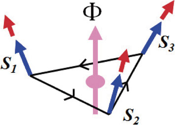
Scalar spin chirality, i.e., the solid angle subtended by the spins, which acts as an emergent magnetic field for the electron coupled to spins. The effective flux Φ penetrating the triangle is given by the product S1 · (S2 × S3).
Therefore, the effective transfer integral, tij, between the two sites i and j is given by
| \begin{equation} t_{ij} = t \langle \chi_{i}|\chi_{j}\rangle, \end{equation} | [15] |
The picture obtained above is that the system is described by the spinful fermions and spinless bosons, which are coupled through the strongly fluctuating gauge field, i.e., the emergent electromagnetic field. By integrating over this gauge field, one can obtain the physical response functions from those of fermions and bosons.11) For example, the resistivity, ρ, of the system is given by the sum of those of fermions, ρF, and bosons, ρB. Since the boson density is that of the doped holes, x, while that of fermions is 1 − x. Therefore, ρB is much larger than ρF. The low-energy bosons are scattered effectively by the gauge field, which results in ρB ∝ T, where T is the temperature.8),9) Other physical observables are obtained by combining the contributions from bosons and fermions, which are different for different quantities. This resolved the dichotomy between the two pictures, i.e., the small number x of hole carriers and the large Fermi surface with Luttinger volume, 1 − x.8),9)
The emergent electromagnetic field discussed in the previous section is fluctuating both quantum mechanically and thermally. The strong coupling nature makes it very difficult to treat the fluctuation on a solid basis. One way is to introduce a fictitious parameter, such as N (number of fermion or boson species), and expand with respect to 1/N, assuming a large N. In this limit, the perturbative treatment of the gauge field fluctuation is justified, while the applicability to the realistic case of N = 2 is not well-founded. Nonperturbative effects, such as confinement, remains an important issue to pursue, which is related to fractionalization of the electrons.6) On the other hand, there are several situations where the emergent magnetic field is static without any fluctuation. In this case, the problem is reduced to that of a single-particle, and one can solve the problem exactly.
The non-collinear spin structures offer an ideal arena to study this possibility. Especially, the non-coplanar spin structure with the solid angle subtended by the spins produces the static emergent magnetic field, leading to the Hall effect.12),13) This possibility was tested in the non-coplanar spin structure in pyrochlore ferromagnet NdMo2O7, where the strong single-spin anisotropy enforces the directions of the rare-earth (Nd) moments to point outward from or inward to the center of the tetrahedron, which are coupled to the conduction electrons of Mo atoms.14) Therefore, the conduction electrons are subject to the emergent magnetic field, and show the anomalous Hall effect. However, note that the periodicity of the electronic state does not change due to the magnetic ordering, and hence the band structure is well defined with the original first-Brillouin zone in this material. Therefore, it is more appropriate to consider the Berry phase of the Bloch wavefunctions in momentum space rather than the emergent magnetic field in real space.
B. Skyrmion.The concept of the emergent electromagnetic field in real space applies well to the spin texture, called skyrmion,15) as schematically shown in Fig. 2. It is realized in a noncentrosymmetric ferromagnet, as observed experimentally by neutron-scattering experiments16) and Lorentz electron transmission microscopy.17) Theoretically, skyrmions are described by the Hamiltonian
| \begin{equation} H_{\text{S}} = \int d^{3}\boldsymbol{{x}}\left[ \frac{J}{2a}(\nabla \boldsymbol{{n}})^{2} + \frac{D}{a^{2}}\boldsymbol{{n}} \cdot [\nabla \times \boldsymbol{{n}}] - \frac{\mu}{a^{3}}\boldsymbol{{H}} \cdot \boldsymbol{{n}} \right], \end{equation} | [16] |
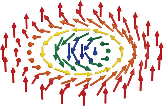
Schematic view of a skyrmion structure. It is a swirling vortex-like spin texture with the spin at the core pointing downward. The spins point in all the directions, which wrap the unit sphere. This is described by the topological index, Q, defined in Eq. [19] in the text.
Therefore, the motion of the skyrmion can be regarded as being classical. The real-space emergent magnetic field due to the spin texture is given by
| \begin{equation} \boldsymbol{{h}} = \boldsymbol{{\nabla}}\times \boldsymbol{{a}} = \frac{\hbar c}{2e}\left( \boldsymbol{{n}} \cdot \partial_{x}\boldsymbol{{n}} \times \partial_{y}\boldsymbol{{n}} \right)\hat{z}, \end{equation} | [17] |
| \begin{equation} e_{i} = - \frac{1}{c}\frac{\partial a_{i}}{\partial t} = \frac{\hbar c}{2e}\left( \boldsymbol{{n}} \cdot \partial_{i}\boldsymbol{{n}} \times \partial_{t}\boldsymbol{{n}} \right). \end{equation} | [18] |
| \begin{equation} Q = \frac{1}{4\pi}\int_{\text{uc}}\,d^{2}\boldsymbol{{xn}} \cdot \left( \partial_{x}\boldsymbol{{n}} \times \partial_{y}\boldsymbol{{n}} \right) = \pm 1. \end{equation} | [19] |
The skyrmion number, Q, cannot be changed by a continuous deformation of the spin configuration, and hence protects the skyrmion topologically. Furthermore, Q enters into the effective action for the center-of-mass motion of a skyrmion as $Q(X\tfrac{dY}{dt} - Y\tfrac{dX}{dt})$, which indicates the canonical conjugate relation between the two components X and Y of the position. This is analogous to the charged particle under the magnetic field, and the velocity becomes perpendicular to the force. This Gyro-dynamics results in the unique motion of the skyrmion, especially under the current. For example, the threshold current density for the spin-transfer torque effect is orders of magnitude smaller than that of the domain wall, because skyrmions avoid the impurity potential due to the Gyro-dynamics.15)
C. Multiferroics.The concept of the emergent electromagnetic field can be generalized to the non-Abelian case. The most natural extension is the SU(2) gauge field corresponding to the spin degrees of freedom. Starting from the Dirac equation, one obtains the effective Lagrangian for the positive energy space by expanding with respect to 1/(mc2), as22),23)
| \begin{align} L &= i\psi^{\dagger}D_{0}\psi + \psi^{\dagger}\frac{\boldsymbol{{D}}^{2}}{2m}\psi\\ &\quad + \frac{1}{2m}\psi^{\dagger}\left[ eq\sigma^{a}\boldsymbol{{A}} \cdot \boldsymbol{{A}}^{a} + \frac{q^{2}}{4}\boldsymbol{{A}}^{a} \cdot \boldsymbol{{A}}^{a} \right]\psi. \end{align} | [20] |
| \begin{equation} P_{i} \propto \epsilon_{ia\ell}j_{\ell}^{a}, \end{equation} | [21] |
Therefore, once the spin ordering produces the spin current, the electric polarization emerges, which offers a mechanism of ferroelectricity of spin origin, i.e., multiferroics.26),27) This mechanism explains well the first discovery of the magnetic control of ferroelectric polarization in manganite.28)
The commutators among the spin components,
| \begin{equation} [S^{\alpha},S^{\beta}] = i\hbar \varepsilon_{\alpha \beta \gamma}S^{\gamma}, \end{equation} | [22] |
| \begin{equation} [S^{z},S^{\pm}] = \pm i\hbar S^{\pm}, \end{equation} | [23] |
| \begin{equation} [S^{z},\theta ] = i\hbar. \end{equation} | [24] |
| \begin{equation} \boldsymbol{{P}} = \eta \boldsymbol{{e}}_{ij} \times (\boldsymbol{{S}}_{i} \times \boldsymbol{{S}}_{j}), \end{equation} | [25] |

Schematic illustration of the spin-current mechanism of the electric polarization. When the spins Si and Sj are tilted, the polarization, P, is induced, as given by P = ηeij × (Si × Sj) (Eq. [25]), with eij being the unit vector connecting the atoms i and j.
The Berry phase of the Bloch wavefunctions in solids is an important issue related to many hot topics in the current condensed-matter physics. The Bloch wavefunction is written as
| \begin{equation} \psi_{n\boldsymbol{{k}}\sigma}(\boldsymbol{{r}},s) = e^{i\boldsymbol{{k}} \cdot \boldsymbol{{r}}}u_{n\boldsymbol{{k}}}(\boldsymbol{{r}})\chi_{\sigma}(s), \end{equation} | [26] |
| \begin{equation} a_{na}(\boldsymbol{{k}}) = - i \langle u_{n\boldsymbol{{k}}}|\partial_{k_{a}}|u_{n\boldsymbol{{k}}}\rangle \end{equation} | [27] |
| \begin{equation} \boldsymbol{{b}}_{n}(\boldsymbol{{k}}) = \nabla_{k} \times \boldsymbol{{a}}_{n}(\boldsymbol{{k}}), \end{equation} | [28] |
This Berry phase modifies the equation of motion for a wave-packet made of the Bloch states.29),30) Due to the canonical conjugate relation, the position operator, x, is usually defined as xμ = i∂/∂kμ. When the wave-packet is made from the subspace characterized by the Berry connection, it should be modified into the gauge covariant form as
| \begin{equation} x_{\mu} = i\partial /\partial k_{\mu} + a_{n\mu}(k). \end{equation} | [29] |
| \begin{align} \frac{dx_{\mu}}{dt} &= - i[x_{\mu},H],\\ \frac{d\pi_{\mu}}{dt} &= - i[\pi_{\mu},H], \end{align} | [30] |
| \begin{align} v_{\mu} &= \frac{dx_{\mu}}{dt} = \frac{\partial \varepsilon_{n}(\boldsymbol{{k}})}{\partial k_{\mu}}|_{\boldsymbol{{k}} + e\boldsymbol{{A}}} - i[x_{\mu},x_{\nu}]\frac{\partial V(\boldsymbol{{x}})}{\partial x_{\nu}}\\ &= \frac{\partial \varepsilon_{n}(\boldsymbol{{k}})}{\partial k_{\mu}} + \varepsilon_{\mu \nu \lambda}b_{\lambda}(\boldsymbol{{k}})\frac{\partial V(\boldsymbol{{x}})}{\partial x_{\nu}}\\ &= \frac{\partial \varepsilon_{n}(\boldsymbol{{k}})}{\partial k_{\mu}} + (\boldsymbol{{b}} \times \boldsymbol{{F}})_{\mu},\\ \frac{dk_{\mu}}{dt} &= - \varepsilon_{\mu \nu \lambda}ev_{\nu}B_{\lambda}(\boldsymbol{{k}}) - \frac{\partial V(\boldsymbol{{x}})}{\partial x_{\nu}} = F_{\mu}, \end{align} | [31] |
Note that there is one sharp difference between the Maxwell magnetic field, B, and Berry curvature, b. Namely, B is divergence-free, i.e., ∇x · B(x) = 0, corresponding to the absence of a magnetic monopole, while ∇k · b(k) can have a magnetic monopole at a band crossing point, as discussed in Eq. [5], with X being replaced by k.
Another important remark is that the symmetries give the following constraint. The time-reversal symmetry, $\mathcal{T}$, gives the relation bn(k) = −bn(−k), while the spatial inversion symmetry, $\mathcal{I}$, gives bn(k) = bn(−k). Therefore, when both $\mathcal{T}$ and $\mathcal{I}$ symmetries are there, and the Berry curvature, bn(k), vanishes. Also, in the noncentrosymmetric system, where $\mathcal{I}$-symmetry is absent, bn(k) can be nonzero, although the contributions from k and −k cancel with each other when $\mathcal{T}$ is intact.
We now discuss the Hall effect driven by the Berry curvature (emergent magnetic field) in momentum space.32) From the above consideration, the Hall conductivity σH is given by the integral of the Berry curvature over the occupied states, i.e.,
| \begin{equation} \sigma_{H} = \frac{e^{2}}{\hbar}\sum_{n}\,\int \frac{d\boldsymbol{{k}}}{(2\pi)^{d}}f(\varepsilon_{n}(\boldsymbol{{k}}))b_{nz}(\boldsymbol{{k}}), \end{equation} | [32] |
| \begin{equation} \sigma_{H} = \frac{e^{2}}{\hbar}\sum_{n\text{occupied}}\oint_{C}\frac{d\boldsymbol{{k}}}{(2\pi)^{2}} \cdot \boldsymbol{{a}}_{n}(\boldsymbol{{k}}) = \frac{e^{2}}{h}\sum_{n\text{occupied}}N_{c} (n), \end{equation} | [33] |
Equation [32] represents the intrinsic Hall effect due to the geometrical nature of the Bloch wavefunctions, which is also applicable to a metallic system. This offers a modern interpretation of the old theory by Karplus-Luttinger for the anomalous Hall effect (AHE) in metallic ferromagnets.34) However, there has been a long-term controversy about the origin of the AHE. After a paper by Karplus-Luttinger, the effects of the impurity scatterings are proposed to be essential for the AHE, and extrinsic mechanisms, i.e., the skew scattering35) and side jump,36) were proposed. A unified theoretical treatment of this issue has recently been developed, and now the respective role of intrinsic and extrinsic mechanisms are now clarified.32) Beyond the perturbative treatment of the spin-orbit interaction, it is now recognized that the band crossings near the Fermi energy play an essential role, and act as the monopoles of the Berry curvature. Therefore, intrinsic Hall conductivity has a topological meaning and is robust against impurity scatterings. Therefore, as a function of the diagonal conductivity, there are three regions of the AHE, i.e.: (i) the strongly disordered case, where the intrinsic contribution is reduced and approximately the relation $\sigma _{H} \propto \sigma _{xx}^{1.6}$ holds, (ii) the intermediate case, where the intrinsic contribution is dominant and σH is almost constant, and (iii) the clean case, where the skew scattering contribution is dominant.
Now first-principles band structure calculations can predict the intrinsic anomalous Hall conductivity with reasonable accuracy to be compared with experiments, and there are several materials where the intrinsic AHE is established. Band structure calculations have revealed many band crossings near the Fermi energy, and their resonant contribution to the Hall conductivities, which is a common feature of ferromagnetic metals.
Also, one can ask if the AHE can be quantized in 2D without an external magnetic field. This issue is related to Haldane’s work on the quantized Hall effect without the Landau levels.37) He introduced the nearest neighbor and next-nearest neighbor hopping integrals, the latter of which is complex. We have shown that the tight-binding model for a ferromagnet with the spin-orbit interaction leads to a similar model showing the non-zero Chern numbers, and proposed the quantized AHE (QAHE).38),39) Recently, QAHE has been predicted and observed in the surface state of a magnetic topological insulator.40),41)
B. Spin Hall effect.A direction to generalize the idea of intrinsic AHE is to consider the spin current instead of the charge current. This corresponds to the generalization of the Berry phase to a non-Abelian group, i.e., the SU(2) gauge field in spin space. Note that this non-Abelian gauge field can be finite, even with both $\mathcal{T}$ and $\mathcal{I}$ symmetries. In the presence of the SU(2) Berry curvature in momentum space, the generalized equation of motion for the wavepacket of the particle with spin is given by ref. 42
| \begin{equation} \frac{d\boldsymbol{{k}}}{dt} = - e\boldsymbol{{E}}, \end{equation} | [34] |
| \begin{equation} \frac{dx_{\ell}}{dt} = \frac{\partial \varepsilon_{n}(k)}{\partial k_{\ell}} - \frac{dk_{j}}{dt}(z^{\dagger}F_{\ell j}^{n}z), \end{equation} | [35] |
| \begin{equation} \frac{dz}{dt} = i\frac{d\boldsymbol{{k}}}{dt} \cdot (\boldsymbol{{A}}^{n}z), \end{equation} | [36] |
| \begin{equation} j_{j}^{i} = \sigma_{s}\epsilon_{ijk}E_{k}, \end{equation} | [37] |
Equation [37] has been explicitly derived for the p-type GaAs, where the 4-fold degeneracy of the band occurs at the Γ-point. It acts as the Yang-monopole, i.e., a generalization of the U(1) monopole to the SU(2) case, and hence the gauge field strength, Fij, is given by
| \begin{equation} F_{ij} \propto \pm \varepsilon_{ij\ell}\frac{k_{\ell}}{k^{3}}. \end{equation} | [38] |
Since the emergent electromagnetic field is not directly related to the real electromagnetic charge, one can expect that it is also relevant to the neutral particles. For example, photon is the constrained system, i.e., the polarization of the electric and magnetic fields are perpendicular to the wavevector, and hence the Berry phase appears. Therefore, one can derive the equation of motion for the wavepacket of the photon, similar to Eq. [36]. This leads to the Hall effect of light, where the shifts of the reflected and transmitted light beams occur transverse to the incident direction with the opposite directions for right and left-circular light.45) Another example is the Hall effect of magnons, where, e.g., the relativistic DM interaction gives the phase factor for the propagation of the magnon, leading to the Berry curvature in momentum space in ferromagnets with multiple atoms in the unit cell.46) The thermal Hall effect in pyrochlore insulating ferromagnet Lu2V2O7 has been analyzed from this viewpoint showing the excellent agreement between the theory and experiment.47)
C. Ferroelectricity and shift current.It is now well known that the Berry phase is relevant to the electronic contribution to the electric polarization.48),49) The idea is to integrate the polarization current over the displacement of the atoms from the symmetric positions. This polarization current is driven by the Berry phase. More explicitly, consider the two-dimensional space of the momentum, kx, and the displacement, D. Adiabatically increasing D(t) from 0 to the physically realized value D(T) = D0, the polarization current is given by the integral over the first Brillouin zone as
| \begin{equation} J_{x}(D) = \int_{-\pi}^{\pi}\,\frac{dk_{x}}{2\pi}F_{k_{x}D}(k_{x},D)\frac{dD}{dt}. \end{equation} | [39] |
| \begin{equation} P(D_{0}) = \int_{0}^{T}\,dtJ_{x}(D(t)) = \int_{-\pi}^{\pi}\,\frac{dk_{x}}{2\pi}A_{k_{x}}(k_{x},D_{0}). \end{equation} | [40] |
Recently, an extension of the ferroelectricity to the nonequilibrium situation has been studied extensively in the field of nonlinear optics. As mentioned in the Introduction, the concept of the Berry phase and the emergent electromagnetic field are useful concepts when the wavefunctions are confined in the manifold in Hilbert space. However, generalization of the geometric phase without the adiabatic limit is possible; see e.g., the paper by Aharonov and Anandan.50) Especially, for the interband transition by high-energy photons, the electrons jump from one manifold to the other. Even in this high-energy process, the concept of the Berry phase is useful. Intuitively, the change in the intracell coordinate associated with the interband transition creates a current, which is called the shift current.51) This shift current can be a dc current by steady photoexcitation, although it is closely related to the polarization current. Namely, the integral of the intracell coordinate over the occupied band is the polarization, and the interband transition partly changes this polarization to result in the current. The reason why it can be the dc current is that the relaxation is “neutral”, i.e., the relaxation has no preferred direction while the excitation is asymmetric between right and left.
This phenomenon can be formulated by the Floquet formalism combined with the Keldysh Green function method. Consider the 2 × 2 Hamiltonian,52)
| \begin{equation} h = \begin{pmatrix} \epsilon_{1}^{0} & iFv_{12}^{0}\\ -iFv_{21}^{0} & \epsilon_{2}^{0} \end{pmatrix} \equiv \epsilon + \boldsymbol{{d}} \cdot \boldsymbol{{\sigma, }}\end{equation} | [41] |
| \begin{equation} - ev = - e\frac{\partial h}{\partial k} \equiv b_{0} + \boldsymbol{{b}} \cdot \boldsymbol{{\sigma.}} \end{equation} | [42] |
| \begin{align} J &= \int dk\frac{\pi E^{2}}{2\Omega^{2}}\frac{\Gamma}{\sqrt{\tfrac{E^{2}}{\Omega^{2}} + \Gamma^{2}}}\delta (d_{z})|v_{12}^{0}|^{2}\\ &\quad\times \left[ \frac{d}{dk}\text{Im}(\log v_{21}^{0}) + a_{22} - a_{11} \right], \end{align} | [43] |
This shift current can be the mechanism of the photovoltaic effect in perovskite materials.53) A first-principles band structure calculation can predict the shift current as a function of the energy of the incident light. For example, a detailed comparison has been done for the photovoltaic effect in BaTiO3, showing a good agreement between theory and experiment.54) This shift current could be relevant to the high-efficiency solar-cell action. Theoretically, the shift current does not require the free carriers analogously to the fact that the polarization current can exist in insulators. Actually, it is proposed theoretically that the shift current remains finite, even when the photon energy is below the particle-hole continuum, i.e., at the exciton absorption peak.55) The shift current can be regarded as being one of the nonreciprocal responses in noncentrosymmetric systems, and a unified understanding of them is an important future problem.56)
The emergent electromagnetic field corresponds to the curvature defined locally at each point of the manifold. It is the most remarkable result in differential geometry that one can derive the topological invariant by the integral of the local curvature over the manifold. The classic example of this fact is the Gauss-Bonnet theorem, where the integral of the Gauss curvature over the closed surface in three-dimensions gives the number of “holes” called genus.1) This wisdom can be applied to the electronics states in solids. The Chen number discussed for the quantum Hall effect is an example of this application.33) The gap protects this topological index, i.e., it remains unchanged as long as the gap does not close. In other words, the gap must close to have any change in the topological index. This leads to the “bulk-edge correspondence”. Namely, the vacuum outside of the solid is a “trivial” state, and the gap must close at the surface when the electronic states inside the solid has a nontrivial topological index. Therefore, the gapless states should appear at the surface or edge of the system, which is protected by the topology of the bulk states.
Looking into a more explicit example, it is a natural question as to whether the analogue of the quantum Hall effect exists also for the SHE. The simplest case is that the spin-up and spin-down electrons are decoupled, showing the opposite sign of the quantized Hall conductance, i.e., quantized spin Hall effect. In general, however, the spin is not conserved in the presence of the spin-orbit interaction and the spin components are mixed. Therefore, it is a highly nontrivial issue as to how to define the quantum SHE in this general case. Actually, it has been revealed by a seminal paper by Kane and Mele57) that one can define the Z2 topological index, which is not related to the spin Hall effect, but is related to the edge channels.58),59) This Z2 index is closely related to the time-reversal symmetry, $\mathcal{T}$, and Kramer’s theorem coming from the fact that $\mathcal{T}^{2} = - 1$ for the half-odd integer spin, S. The helical edge channel remains gapless as long as the perturbations, such as the impurity scattering respect the time-reversal symmetry, $\mathcal{T}$. Namely, the crossing of the dispersion of the helical edge channel is the Kramer’s doublet at the time-reversal symmetric momentum.
This two-dimensional quantum SHE was the first discovery of topological insulators (TI’s), which are now fully classified by K-theory in any dimensions and symmetry classes.58),59) The three-dimensional TI has no analogue to the quantum Hall system. It is characterized by the surface gapless Weyl fermion with the spin and momentum locked, as observed by the spin-resolved ARPES experiment.58) This corresponds to half of the Dirac fermion, i.e., an example of the electron fractionalization. This momentum-spin locking corresponds to the strong coupling limit of the spin-orbit interaction, and is hence expected to be very useful in spintronics applications. Especially, when magnetization normal to the surface is introduced, there appears a gap of the surface Weyl fermion. This is a system showing the parity anomaly in two-dimensions, which shows the Hall conductance, e2/(2h). When the magnetization direction is the same for both the top and bottom surfaces, the Hall conductance of the total system is e2/h with the chiral edge channel circulating along the side surface. This is an ideal laboratory to realize the quantized anomalous Hall effect predicted theoretically. Actually, it was discovered experimentally in 2013 in magnetically doped TI Cr:Bi2Te3, as discussed above.41) It has been also proposed that the magnetic surface of TI behaves as a two-dimensional multiferroics.60)
We have reviewed physical phenomena related to emergent electromagnetism in solids. They are all related to the geometrical properties of the wavefunctions on the manifold in Hilbert space. The gauge field naturally and ubiquitously appears when the system is constrained, and the nontrivial geometry is possible accordingly. This gauge field is called an “emergent electromagnetic field” analogously to the Maxwell electromagnetic field.
The emergent electromagnetic fields are classified into those in real space and momentum space, but they can be unified into the phase space, i.e., 6-dimensions including both the real and momentum spaces. Furthermore, adding the parameters characterizing the Hamiltonian, one can consider the even higher dimensional spaces providing much richer structures of theories. Actually, in cold atom systems, the “synthetic dimensions” is designed to realize e.g. the four-dimensional quantum Hall state.
Another future direction is to consider the time-dependence of the emergent electromagnetic field more. Especially, the dynamics of the emergent electromagnetic field in momentum space has not been yet explored very much thus far. There remain many interesting and important problems related to emergent electromagnetic field to be studied in the future, which will provide a more coherent and unified view of the electronic systems in solids.
The author thanks A.V. Balatsky, H.J. Han, J. Iwasaki, C. Jia, H. Katsura, W. Koshibae, P.A. Lee, M. Mochizuki, T. Morimoto, M. Mostovoy, S. Murakami, K. Nomura, M. Onoda, S. Onoda, J. Zang, S.C. Zhang, for collaborations, and Y. Tokura, T. Arima, M. Kawasaki, Y. Iwasa for useful discussion. This work was supported by JSPS KAKENHI Grant (Nos. 18H03676, 26103006), and by JST CREST Grant Number JPMJCR1874, Japan.

Naoto Nagaosa was born in Hyogo Prefecture in 1958, and graduated from Department of Applied physics, The University of Tokyo in 1980. From 1983 to 1986, he was a research associate in Institute for Solid State Physics, Univ. Tokyo, and received a D.Sci from Univ. Tokyo in 1986. From 1988 to 1990, he worked as a visiting scientist at Department of Physics, Massachusetts Institute of Technology, before joining the Department of Applied Physics in Univ. Tokyo where he is now a professor. From 2013 he has joint appointment with the Deputy Director of the RIKEN Center for Emergent Matter Science (CEMS). His research field is theoretical condensed-matter physics, especially involving the strong electron correlation, optical responses of solids, topological aspects of condensed matter, and superconductivity. For his accomplishments, he has received the Yukawa Prize, Japan IBM Prize, Nissan Science Prize, Nishina Memorial Prize, Fujihara Award, and Medal with Purple Ribbon.