Review
Cold and stable antimatter for fundamental physics
2020 年 96 巻 10 号 p. 471-501
詳細
2020 年 96 巻 10 号 p. 471-501
The field of cold antimatter physics has rapidly developed in the last 20 years, overlapping with the period of the Antiproton Decelerator (AD) at CERN. The central subjects are CPT symmetry tests and Weak Equivalence Principle (WEP) tests. Various groundbreaking techniques have been developed and are still in progress such as to cool antiprotons and positrons down to extremely low temperature, to manipulate antihydrogen atoms, to construct extremely high-precision Penning traps, etc. The precisions of the antiproton and proton magnetic moments have improved by six orders of magnitude, and also laser spectroscopy of antihydrogen has been realized and reached a relative precision of 2 × 10⁻¹² during the AD time. Antiprotonic helium laser spectroscopy, which started during the Low Energy Antiproton Ring (LEAR) time, has reached a relative precision of 8 × 10⁻¹⁰. Three collaborations joined the WEP tests inventing various unique approaches. An additional new post-decelerator, Extra Low ENergy Antiproton ring (ELENA), has been constructed and will be ready in 2021, which will provide 10–100 times more cold antiprotons to each experiment. A new era of the cold antimatter physics will emerge soon including the transport of antiprotons to other facilities.
The Low Energy Antiproton Ring (LEAR) at CERN, constructed in 1982 and operated until 1996, triggered a break for a cold antimatter science,1) which flowered during the Antiproton Decelerator (AD) time.2) It is expected to grow further waiting for the start of the operation of the Extra Low ENergy Antiproton ring (ELENA) in 2021 (see §4). Cold antimatter science is thus a relatively young research field of physics that focuses primarily on fundamental physics, but at the same time on multidisciplinary science covering nuclear physics, atomic physics, plasma physics, as well as a basic study on cancer therapy.3) The field has been becoming active more than ever while growing its population and contributing to fundamental physics via high-precision measurements, which has been particularly true during the last 10 years.
Cold antimatter science has two major topics: one is CPT symmetry tests that compare proton (p) and antiproton ($\overline{\text{p}}$), hydrogen (H) and antihydrogen ($\overline{\text{H}}$) as well as antiprotonic helium ($\overline{\text{p}}$He+), where C, P and T refer to charge conjugation, parity, and time reversal, respectively; the other one is the Weak Equivalence Principle (WEP) tests that measure the gravitational interaction between antimatter ($\overline{\text{H}}$) and matter (the Earth). The key property of $\overline{\text{p}}$ and $\overline{\text{H}}$ which enable to attack the above subjects is their stability, which exclusively enables one to conduct high-precision measurements.
CPT symmetry is naturally concluded from the Standard Model (SM), the most successful theoretical framework of fundamental physics. On the other hand, recent important discoveries in this field of physics as well as astronomy are not well settled in the framework of the SM. Examples of such discoveries include neutrino oscillation,4) dark matter, and dark energy. It is also noted that the gravitational interaction is not in the scope of the SM. Considering these, although speculative, CPT symmetry and WEP tests have been selected as the major subjects, which may also shine a light in the mystery of a matter-dominant universe (see e.g., Refs. 5–7).
The universe is believed to have contained the same amount of matter and antimatter at the moment of the Big Bang according to the best knowledge of the present elementary particle physics. However, it looks like the present universe favors matter. Every effort to find celestial antimatter has been unsuccessful until now, strongly indicating that the production and/or annihilation processes are asymmetric between matter and antimatter in some way. For example, the AMS project, which measures various particles showering on Earth found eight antihelium events (six of them were compatible to $\overline{^{3}\text{He}}$ and the rest of two were $\overline{^{4}\text{He}}$), which were ∼10−8 of helium events during the six years of continuous measurements.8),9) The possibility of a matter-antimatter patchwork universe was also discussed,10) and it was concluded that the size of the patch would be comparable to that of the observable universe, i.e., a matter-antimatter symmetric universe is unfavored. What happened to all of the antimatter?11)
The most recognized model to explain a matter-dominant universe was proposed by Sakharov in 1967,12) which requires three conditions: baryon number non-conserving processes, C- and CP-violations, and interactions under non-equilibrium conditions. Actually, CP symmetry is experimentally found to be violated for K- and B-mesons (see also §2.3). It is noted that baryon number non-conserving processes have not yet been found experimentally, and also need further theoretical study. It is also noted that SM has been constructed so that P, T, and CP violation can be built in “by hand” with many free parameters, but is not necessarily delivered from first principles with a few parameters.13)
Astrophysical observations have revealed that the amount of matter left in the present universe resulted from a tiny difference between matter and antimatter, ∼10−9.14) This tiny asymmetry is, however, by far too large to be explained by the known CP violation in the quark sector by a factor of 109, and this huge factor still has no reasonable explanation. Due to this level of asymmetry, we human beings are fortunately here on a tiny planet of the Solar system in a countryside of the Milky Way galaxy, one of 1012 galaxies, and now seriously discussing why and how we survived from full annihilation while developing a high-precision science (see Fig. 1).

(Color online) After 13.8 billion years from the Big Bang, we human beings are here on Earth, wondering why we exist longing for anti-human beings somewhere in the universe.
Cold antimatter physics is expected to provide a new path to study fundamental physics via high-precision measurements, while realizing lower than ever in temperature, which is in good contrast to the traditional “high energy physics” pushing higher than ever in energy. For example, a high-precision laser spectroscopy has already achieved an amazing precision, as high as Δν/ν = 10−18, and is still improving. This provides an excellent tool to study fundamental physics in the low energy regime,15),16) which would have a good overlap with the cold antimatter physics discussed here. It is also noted that the Large Hadron Collider (LHC), the biggest accelerator in the world, is already ∼10−3 of the size of Earth. Although this direction can still be kept, it would also be the time to consider alternative schemes as well.1
This review is organized in the following way: In §2, the backgrounds of cold antimatter research are described referring to foregoing research on the CPT symmetry and Weak Equivalence Principle. §3 gives a short history of cold antimatter research during the LEAR time before the AD operation. §4 discusses how to prepare cold antiprotons. §5 explains various experimental schemes to synthesize antihydrogen atoms and how to manipulate them for physics experiments. In §6, several latest achievements on high-precision spectroscopy with antiprotons and antihydrogen atoms are discussed. §6.3 is for unique and exotic atoms, $\overline{\text{p}}$He+ and its high-precision laser spectroscopy. §7 explains three ongoing experiments aiming to directly measure the gravitational interaction between antimatter (antihydrogen) and matter (Earth). §8 considers other topics related to experiments at the AD as well as a couple of additional possible subjects. Finally, §9 provides a summary and considers the future.
Symmetries are an essential concept in modern physics, particularly in the SM, and are categorized into global and local symmetries, which are related to conservation laws and forces, respectively.18) Charge conjugation (C), parity operation (P), and time reversal (T) are the components of discrete symmetry transformations. CPT symmetry, simultaneous applications of all three transformations, is supposed to be the most fundamental symmetry in modern physics. The SM originally developed by Lueders,19) Pauli,20) Bell,21) and Jost22) is based on local quantum field theory on a flat space-time, fulfilling Lorentz invariance and unitarity. When these conditions are met, a quantum field theory is invariant under the CPT transformation. It is noted that e.g., P,23) CP,24) and T25) have already been found to be violated.
Theoretically, various possibilities to violate the CPT symmetry have been investigated. For example, it was discussed for infinite component fields.26) String theory is in its nature non-local, which can accommodate CPT violation.27) Lorentz invariant non-local CPT violating models are discussed in Refs. 5 and 28. It was also argued that curved space-time due to general relativity may violate CPT symmetry.29) In considering the CPT violation related to the gravitational interaction, the Planck mass, given by mPL = (ħc/G)1/2(∼1019 GeVc−2), where ħ is the Planck constant divided by 2π, and G the gravitational constant, could be a possible measure because it distorts space-time so seriously that the particle with the Planck mass becomes a black hole. The level of the CPT violation could be estimated by the ratio of the mass (m) of the particle in question and the Planck mass, i.e., Rm = m/mPL, which is ∼10−19 for a proton/antiproton. In the energy scale, $m_{\text{p}(\overline{\text{p}})}c^{2}R_{m_{\text{p}(\overline{\text{p}})}} \sim 10^{ - 19}$ GeV ∼ 10 kHz.30)
Important consequences of CPT symmetry are that the mass, total lifetime, absolute charge and magnetic moment of an antiparticle should be exactly the same as those of the corresponding particle. In addition, the spectroscopic properties of complex antiparticle systems (e.g., antihydrogen) should again be identical to the corresponding complex particle systems (e.g., hydrogen). In order to conduct high-precision measurements, it is then essential to adopt stable and controllable systems, in which case, the observation time can be infinitely long, and accordingly, the mass/energy, charge, etc. of the particle pairs in question can be studied in principle with arbitrarily high-precision.
It is also commented that in usual high-precision measurements, experimental results are compared with predictions of precise and reliable theories that take into account all known interactions, in an attempt to find some deviations. The residue, if successfully identified, can be attributed to unknown interactions and/or some unexplored dynamics. CPT symmetry tests are conceptually different. Research can be conducted purely experimentally, without contributions from precise and detailed theoretical predictions. Once any tiny difference between matter and antimatter is observed regarding the quantities described above, it is immediately proof of the violation of the CPT symmetry, pointing to new physics beyond SM. The finding may also lead to a new understanding of the missing antimatter. A drawback, however, is the fact that there are no clear guidelines to suggest appropriate quantities to be measured and the level of necessary precision to detect the difference, because no quantitative theoretical predictions are available. In this respect, the Standard Model Extension (SME) quickly described in the next section provides possible guidelines on what to measure.
2.2. Standard Model Extension (SME).Kostelecký and his colleagues developed a so-called Standard Model Extension (SME), and tried to figure out measurable physical quantities sensitive to the CPT violation by artificially adding CPT and Lorentz-violating operators to the standard CPT conserving Lagrangian of the SM.31),32) For free H/$\overline{\text{H}}$, the modified Dirac equation is given by
| \begin{align} &\bigg(i\gamma^{\mu}D_{\mu} - m_{e} - a_{\mu}^{e}\gamma^{\mu} - b_{\mu}^{e}\gamma_{5}\gamma^{\mu} - \frac{1}{2}H_{\mu\nu}^{e}\sigma^{\mu\nu} \\ &\quad + ic_{\mu\nu}\gamma^{\mu}D^{\nu} + id_{\mu\nu}^{e}\gamma_{5}\gamma^{\mu}D^{\nu}\bigg)\psi = 0. \end{align} | [1] |
For example, the 1S and 2S energy levels of H have the same energy shifts in the leading order, i.e., the 1S-2S transition energy is not influenced by the above terms. The situation is the same for $\overline{\text{H}}$, i.e., the 1S-2S transition is not favored for the CPT symmetry test from the SME viewpoint. On the other hand, e.g., one of hyperfine transition energies of the ground state H is found to be different from that of $\overline{\text{H}}$ in the leading term, i.e., sensitive to CPT violating interactions.32) Sidereal variations are also expected to appear because of the Lorentz violating interactions. It also indicates that comparing quantities in the energy scale is often straightforward to discuss the level of the CPT violation. The SME has been further extended to nonminimal sector for various specific targets.33)–35)
2.3. Foregoing experiments on the CPT symmetry.The magnetic moments of the electron and positron, μ(e−) and μ(e+), were measured in 1987, and were found to be 1 + μ(e+)/μ(e−) = (−0.5 ± 2.1) × 10−12, which is one of the best in the lepton sector.36) Another well-known example is the comparison between K0 and $\overline{\text{K}^{0}}$, the system the CP violation was discovered for the first time.37),38) It was reported in 1995 that the CPT symmetry regarding their mass is conserved with the relative precision, $|m_{\text{K}^{0}} - m_{\overline{\text{K}^{0}}}|/m(\text{K}^{0}) < 6 \times 10^{ - 19}$, often cited as the best CPT symmetry test. In obtaining the above value, $|m_{\text{K}^{0}} - m_{\overline{\text{K}^{0}}}|$ was evaluated from the CP-violating parameters and other measurements, and then was divided by the kaon mass determined by other experiment.38) It is commented in Ref. 39 that the very small quantity above reflects the fact that the CPT violating interaction is very weak compared to the strength of the QCD, and it would be more appropriate to compare with the CP violation level. The CP violation was also discovered in B mesons.40),41)
Like in the case of the kaon CPT symmetry discussion above, relative precisions are often referred to. Let’s consider as an example, the spectroscopy of the 1S-2S transition of hydrogen atoms. It is reported that Δν1S-2S/ν1S-2S = 4.2 × 10−15.42) The relative precision reflects e.g., an intrinsic nature of the measured quantity (like its lifetime) as well as the technical level of the corresponding measurement scheme. When we compare different quantities, however, we should be careful. Let’s take the case of the hyperfine transition of atomic hydrogen in its ground state. The best reported value is ΔνHF/νHF = 6.3 × 10−13.43),44) Apparently, the relative precision of ΔνHF/νHF is poorer by two orders of magnitude than that of Δν1S-2S/ν1S-2S. If however the precisions are compared in the energy scale, ΔνHF ∼ 9 × 10⁻⁴ Hz and Δν1S-2S ∼ 10 Hz, i.e., the hyperfine transition is four orders of magnitude better known than the 1S-2S transition. Of course, the figure of merit should be carefully examined case by case as was discussed concerning the CPT-violating coefficients in §2.2.
Following the argument above, the CPT symmetry between K0 and $\overline{\text{K}^{0}}$ expressed in energy scale is $|m(\text{K}^{0}) - m(\overline{\text{K}^{0}})| < 4 \times 10^{ - 19}$ GeV ∼ 105 Hz. Comparing this quantity with those of hydrogen spectroscopy (∼10 Hz/10−3 Hz), it is attractive to challenge the antihydrogen spectroscopy for a serious test of the CPT (see §6.1 for the latest result).
2.4. Weak Equivalence Principle.The Weak Equivalence Principle (WEP) states that the trajectory of a free-falling object is independent of its composition and structure, which has been tested to very high-precision for a range of material compositions. However, no such precision test has ever been done between matter and antimatter. It is also noted that no theory has ever succeeded in combining quantum physics, which predicts antimatter, with general relativity.
A comparison of the cyclotron frequencies of an antiproton and a proton in the same magnetic field at the same gravitational potential could also give an indirect constraint, assuming the CPT symmetry at zero gravitational potential, which is discussed in §6.2. Only a few direct constraints have been known until now. One was on the arrival time difference of antineutrinos and a neutrino from supernova SN1987a, which is consistent with the Einstein equivalence principle to 1 × 10−6.45) Another one was on the search for gravitationally caused decoherence in the (mixed matter-antimatter) K0-$\overline{\text{K}^{0}}$ system,46) which showed no correlation with the gravitational potential. It would then be highly attractive to make such a direct test using $\overline{\text{H}}$ atoms and Earth as the experimental system.47)
As soon as antiprotons were discovered in 1955,48) various experiments started to use antiprotons as a secondary beam. The difficulties at that time originated from the low production cross section of antiprotons, as compared with lighter particles with the same charge polarity and momentum, like negative pions and electrons. When antiprotons were extracted as a secondary beam, this was practically a pion (and electron) beam with a small fraction of antiprotons with the same momentum.1) The application of the storage ring to a secondary beam together with the cooling techniques drastically improved the situation. Pions fully disappear during the macroscopic storage time in the ring and electrons, if any, lose their energies via synchrotron radiation leaving a pure antiproton beam in the ring. The stochastic and electron cooling techniques opened for the first time a chance to even decelerate a beam while keeping its quality and the number of particles.3
The Low Energy Antiproton Ring (LEAR) was built in 1982 and operated until 1996.1) In 1986, Gabrielse reported the first capture of antiprotons in a Penning trap for 100 s using 21 MeV antiprotons from the LEAR (Experimental#:PS-196).50) In the same year, the first atomic collision experiment with antiprotons was reported by the atomic collision group of Aarhus University concerning the ionization of He. The results received a big surprise in the community because the double ionization cross section for antiprotons of several MeV is about two times bigger than that of the same speed protons at collision velocities much higher than the orbital velocity of electrons in He (PS-194).51) It took almost 20 years to theoretically solve this interesting observation.52)
Research topics related to the scope of this review during the LEAR time are the following (see https://en.wikipedia.org/wiki/List_of_Proton_Synchrotron_experiments): In 1988, antiprotonic X-rays from $\overline{\text{p}}^{108}$Pb were measured, and the magnetic moment of $\overline{\text{p}}$ was evaluated to be $\mu _{\overline{\text{p}}} = - 2.8005(90)$ μN (PS-186).53) Measurements of the gravitational acceleration of antiproton was proposed in 1986 by Nieto and Holzscheiter (PS-200). In 1989, Y. Yamazaki proposed measurements of wake-riding electrons by employing antiprotons travelling through a carbon foil in collaboration with the Aarhus group (PS-204).54) In 1991, T. Yamazaki proposed a laser spectroscopy of antiprotonic helium ($\overline{\text{p}}$He+), following the discovery of metastable $\overline{\text{p}}$He+s.55) This subject has been quite productive and is still actively in progress, as is discussed in §6.3 (PS-205).56),57) Gotta proposed to measure Lyman- and Balmer-transitions of $\overline{\text{p}}$p and $\overline{\text{p}}$He++ (PS-207). Jastrzebski proposed to study the neutron halo with antiprotonic X-rays (PS-209) (see §8.1). As is discussed in §5.1, Oelert proposed the formation of fast $\overline{\text{H}}$s using relativistic $\overline{\text{p}}$s colliding with a gaseous target (PS-210), and succeeded for the first time in identifying eleven $\overline{\text{H}}$s.58)
LEAR was closed in 1996, and the construction of a low-cost successor, Antiproton Decelerator (AD), was discussed and approved. AD started operation in 2000, and is still stably running as the central facility of cold antimatter research, expanding the number of user groups, as described in §4.1. Figure 2 shows all of the experiments at AD approved and to be approved. At the start of AD operation, three experiments were proposed and approved in 1997: the AnTiHydrogEN Apparatus (ATHENA) experiment, the Antiproton TRAP (ATRAP) experiment (concluded in 2018), and the Antiproton Spectroscopy And Collisions Using Slow Antiprotons (ASACUSA) experiment. The main subject of the ATHENA experiment was antihydrogen synthesis and precision measurements. On the other hand, the ATRAP experiment aimed at both antihydrogen synthesis as well as high-precision measurements of $\overline{\text{p}}$s. The ASACUSA experiment consisted of two major groups when it started, i.e., the antiprotonic helium spectroscopy group (ASACUSA-$\overline{\text{p}}$He) and the atomic collision group. The latter added another major subject, antihydrogen spectroscopy adopting a unique idea, a so-called cusp trap that enables one to focus an antihydrogen beam into a magnetic field-free region59) (see §5.2) from 2003 (ASACUSA-Cusp). The ASACUSA experiment has been from the beginning very unique in the sense that the research subjects were more distributed rather than concentrated, also including nuclear physics experiments. From 2004, the Antiproton Cell Experiment (ACE) joined to study the feasibility of using antiprotons for cancer therapy. This experiment was concluded in 2013. The ATHENA experiment was completed in 2004, and a new experiment, the Antihydrogen Laser PHysics Apparatus (ALPHA) experiment, started from 2008 focusing on antihydrogen trapping and spectroscopy. The ALPHA experiment later added the WEP research as their second subject. In 2014, one more experiment emerged from the former ATHENA members, Antihydrogen Experiment: Gravity Interferometry Spectroscopy (AEgIS), which primarily focuses on the gravitational interaction of antihydrogen with Earth. Further, the Gravitational Behaviour of Antihydrogen at Rest (GBAR) joined also proposing the WEP research, and is waiting for ELENA operation to start from 2021. The last one is the Baryon Antibaryon Symmetry Experiment (BASE), which joined from 2014 focusing on the high-precision measurements of the antiproton charge-to-mass ratio and the magnetic moment. A new experiment, the antiProton Unstable Matter Annihilation (PUMA) experiment, was proposed in 2019, which should be approved sometime soon (see §8.1).

(Color online) Chronological list of all proposed experiments during the AD time (dark-blue bars, running period; light blue bars, period from the approval until the start of the experiment). The five stars show several pioneering studies during the LEAR time. $ \star $1 (1986), first antiproton trapping50); $ \star $2 (1986), first atomic collision with slow antiprotons51); $ \star $3 (1988), magnetic moment measurement of antiprotons (using X-rays from $\overline{\text{p}}$Pb)53); $ \star $4 (1994), first laser spectroscopy of $\overline{\text{p}}$He+57); and $ \star $5 (1996), first observation of fast $\overline{\text{H}}$s.58)
Antiprotons are produced via a nuclear reaction involving the pair production of an antiproton ($\overline{\text{p}}$) and a proton (p), like
| \begin{equation} \text{p} + \text{p}/\text{n} \to \overline{\text{p}} + \text{p} + \text{p} + \text{p}/\text{n}. \end{equation} | [2] |

(Color online) Simplified drawing of the AD (right panel) and the ELENA (left panel). First, 3.6 GeV/c $\overline{\text{p}}$s are injected from the top left of the AD. After cooling and deceleration, 100 MeV/c (5.3 MeV) $\overline{\text{p}}$s are transported to the ATRAP, ASACUSA, ALPHA, BASE, and AEgIS experiments. Once ELENA (left) is ready, a 5.3 MeV beam is injected in ELENA and then decelerated down to 100 keV $\overline{\text{p}}$s, and distributed to these experiments. Test beams from ELENA were transported to the GBAR in 2018.
The right half of Fig. 3 shows a drawing of the AD (circumference of 182 m). A 3.6 GeV/c pulsed $\overline{\text{p}}$ beam injected from the top-left of the ring is guided, cooled and decelerated down to 100 MeV/c (5.3 MeV/u) via the following four steps:
Until 2018, the 5.3 MeV/u $\overline{\text{p}}$s were pulse-extracted from AD with the intensity of a couple of 107 every ∼100 s to one of the experiments, while switching from one experiment to the other every 8 hours, 24 hours a day, 7 days a week for a half year every year. In each experiment except for ASACUSA, the $\overline{\text{p}}$ beam was directly injected in an accumulation trap via a relatively thick foil (∼70 mg/cm2) for degradation. Actually, a large fraction of $\overline{\text{p}}$s was lost in the foil, and only a small fraction of the transmitted $\overline{\text{p}}$s was in a proper energy range (<10 keV) for trapping. This was a simple and reliable technique to slow down the antiprotons at the cost of a low trapping efficiency, typically in the range of 104 $\overline{\text{p}}$s per an AD shot, i.e., 99.9% of the $\overline{\text{p}}$s were abandoned (see §4.4). In the case of ASACUSA, a Radio Frequency Quadrupole Decelerator (RFQD) was developed in collaboration with the CERN RF group, and was used until 2018, which delivered several million $\overline{\text{p}}$s at ∼60 keV (see §4.2), two orders of magnitude higher in efficiency than the thick degrader foil scheme.
4.2. Radio Frequency Quadrupole Decelerator (RFQD).In the case of the ASACUSA experiment, a 5.3 MeV beam of $\overline{\text{p}}$s was injected into the RFQD (the small vertical yellow box at the end of the ASACUSA beamline in Fig. 3). RFQD is 3 m long and decelerates the 5.3 MeV beam from AD down to 63 keV with a deceleration efficiency as high as ∼25%.63) The electrodes of the RFQD were electronically floatable by ∼ ±60 kV, and RFQD was practically an energy-variable decelerator in the range of 10–120 keV. Several ten keV pulsed antiprotons were either transported to a Multi-Ring Electrode trap (MRE, Penning trap) for accumulation and manipulation (to synthesize $\overline{\text{H}}$ atoms or to make atomic collisions) or to a cryogenic target cell filled with 4He or 3He gas/liquid for $\overline{\text{p}}$He+ laser spectroscopy (§6.3). About 1–1.5 million antiprotons were trapped per the AD shot, and stacked when necessary (see §5.2). In the case of atomic collision experiments, antiprotons so accumulated were extracted as a semi-continuous beam at several hundred eV (see §4.5).64),65) The number of antiprotons available for the ASACUSA experiment was thus one to two orders of magnitude larger than that for other experiments.66)
4.3. Extra Low ENergy Antiproton ring (ELENA).The more the antihydrogen research progresses, the more are the demands to increase the number of low energy antiprotons available for experiments. As a drastic solution, a new decelerator ring with a circumference of ∼30 m, the Extra Low ENergy Antiproton ring (ELENA), was decided to be added downstream of the AD, and is now under commissioning at CERN (see Fig. 3).67) ELENA accepts the 5.3 MeV $\overline{\text{p}}$ beam from AD, and then electron-cools and decelerates down to 100 keV in 25 s or so. ELENA is expected to be ready in 2021 shortly after LS2 (long shut down of the CERN accelerator complex starting from the end of 2018).
Antiprotons in ELENA are going to be divided into four bunches that include about 5 × 10⁶ $\overline{\text{p}}$s each. The four bunches are then transported to four different experiments one by one in an on-demand distribution mode. In this way, the number of available antiprotons for each experiment is expected to increase by a factor of ∼10 for ASACUSA and ∼100 for the other experiments. All of the focusing and steering elements of the beam transport lines from ELENA to all of the experiments are designed to be electrostatic.
Table 1 summarizes the main beam parameters of AD and ELENA.
| Parameter | ADinject | ADeject | ELENA |
|---|---|---|---|
| Momentum/ Energy | 3.6 GeV/c | 100 MeV/c (5.3 MeV) | 100 keV |
| (h-/v-) Emittance | 200π mm mrad | 0.3 πmm mrad | 6/4 mm mrad |
| Beam intensity | ∼5 × 10⁷ | 3 × 10⁷ | (5 × 106) × 4 |
| Momentum width ($\frac{\Delta p}{p}$) | 0.06 | 1 × 10⁻⁴ | 2.5 × 10⁻³ |
| Pulse width | 100–200 ns | 100 ns |
Figure 468) shows a schematic drawing of an antiproton trapping and cooling setup of the ASACUSA-Cusp experiment as a typical configuration to dynamically trap $\overline{\text{p}}$s.4 An electron cloud of ∼108 electrons is preloaded in a shallow well prepared near the center of the Multi-Ring Electrode trap (MRE, Penning trap) in a superconducting solenoid.
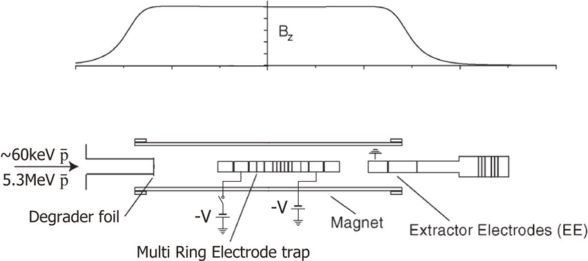
A schematic drawing of the antiproton trapping in a Penning trap.68)
For a charged particle with its charge e and mass m in a magnetic field B, it’s transverse energy will reach its thermal equilibrium with the surrounding electrodes via synchrotron radiation with a damping constant, γrad, given by
| \begin{equation} \gamma_{\textit{rad}} = \frac{\mu_{0}e^{4}B^{2}}{3\pi m^{3}c}\quad(\gamma_{\textit{rad}}^{e^{\pm}}[\text{s}^{-1}] \sim 0.4B[\text{T}]^{2}). \end{equation} | [3] |
As is shown in Fig. 4, a pulsed $\overline{\text{p}}$ beam from the RFQD was guided to the MRE via a thin degrader foil. Antiprotons with an energy range of ∼15 keV or lower were radially confined by a magnetic field of 2.5 T, guided along the trap axis, and then reflected by a high negative voltage (−V) applied to an electrode near the downstream end of the trap. Before the reflected beam traveled back to the upstream end of the MRE, a high negative voltage (−V) was applied, and antiprotons were thus dynamically trapped. The trapped antiprotons oscillating in the MRE were sympathetically cooled via collisions with the preloaded electrons. Electrons heated by the incoming antiprotons were cooled again via synchrotron radiation (Eq. [3]). Such heating and cooling dynamics were visualized in 2005 for the first time by the ASACUSA-Cusp experiment observing the time evolution of the power spectrum of the electron plasma, as shown in Figs. 5(a) and (b) for (2,0) and (3,0) electron plasma modes, respectively.68) When pulsed antiprotons were injected at t = 0, the electron plasma was heated and its plasma mode frequencies increased for a few seconds, and then slowly returned to the original frequencies in a couple of ten seconds, which was much slower than expected from Eq. [3], due to electron-electron collisions and a cavity QED effect. The maximum temperature increase of the electron plasma in this case was evaluated to be ∼0.6 eV based on the frequency shifts.75)

Time evolution of the power versus frequency spectrum of the electron plasma after antiproton injection at t = 0 for (a) the (2,0) and (b) the (3,0) modes. The magnetic field strength was 2.5 T.68)
It is noted that the rotation direction for the oppositely charged plasma is also opposite. However, when e.g., a small amount of $\overline{\text{p}}$s are mixed with an oppositely charged positron plasma, the $\overline{\text{p}}$s rotate in the same direction as the positron plasma with a similar frequency. As a result, each $\overline{\text{p}}$ in the positron plasma inevitably possesses kinetic energy proportional to the square of the distance r from the rotation axis, which amounts to $E_{\overline{\text{p}}}^{r}[\text{K}] \sim (7 \times 10^{ - 11}\rho _{\text{e}^{ + }}[/\text{m}^{3}]\ r[\text{m}]/B[\text{T}])^{2}$ even when the internal temperature is 0. This motion is not negligibly small for a high $\rho _{\text{e}^{ + }}$ and a large r when cold $\overline{\text{H}}$s are synthesized by mixing $\overline{\text{p}}$s and e+s in the nested trap, which is particularly so in producing cold $\overline{\text{H}}$ beams (see §5.1).
By employing the same plasma compression technique, the ASACUSA-Cusp experiment succeeded in compressing a pure $\overline{\text{p}}$ cloud from 3.4 mm down to 0.25 mm in its radius.76) Actually, this was the first observation of a plasma-like behavior of an antiproton cloud.
The temperature of synthesized $\overline{\text{H}}$s, the key parameter of all ongoing antihydrogen experiments, is practically the temperature of the $\overline{\text{p}}$ cloud at the moment of $\overline{\text{H}}$ formation, which is pre-determined by the temperature of the electron cloud used to cool antiprotons. Practically, the temperature of an electron plasma is typically at around 100 K, although its environmental temperature is around the liquid helium temperature (∼4.2 K), probably due to external electronic noise. To realize a lower temperature, the evaporative cooling technique, which was successfully developed for neutral particles to realize Bose-Einstein condensation,77),78) was applied for trapped antiprotons, and a temperature as low as 9 K was achieved by the ALPHA experiment.79)
To push further, the sympathetic cooling of antiprotons by laser-cooled Be+ ions is in progress.80) To avoid annihilation between $\overline{\text{p}}$ and Be+, they should be spatially separated, but at the same time, electronical coupling via induced currents should be strong enough so that the $\overline{\text{p}}$s can be efficiently cooled.
4.5. Application of low energy $\overline{\text{p}}$ beam.The RFQD enabled one to store a large number of $\overline{\text{p}}$s in the MRE, which made it possible for the first time to generate an ultra-low energy quasi-DC beam (a couple of hundred eV) of $\overline{\text{p}}$s in 2003.81) This was done by slowly dripping $\overline{\text{p}}$s from the MRE and transporting them to a magnetic-field-free region through x and y deflectors and electrostatic lenses with three differential pumping stages separated by small variable apertures. In this way, atomic collisions of antiprotons with a gaseous target were realized. The number of antiprotons transported to the end of the differentially pumped beam line was typically 6–7 × 10⁵ per one AD shot. The $\overline{\text{p}}$ beam was then accelerated to targeted energies of 3–25 keV for atomic collisions with He/Ar65) and H2.82) The $\overline{\text{p}} + \text{He}$ collisions were studied at energies as low as 250 eV.83)
The direct beam from RFQD opened a chance to study the stopping power of $\overline{\text{p}}$s in the energy range of 100 keV and lower for the first time. The stopping power of $\overline{\text{p}}$s for metallic targets like C, Al, Ni, and Au were found to be proportional to the $\overline{\text{p}}$ velocity, which is consistent with theoretical predictions that the effective number of electrons contributing to the stopping power is proportional to the projectile velocity.84) The measurements were later extended to an insulating target, LiF (the bandgap is ∼10 eV), expecting different behaviours. Surprisingly, the stopping power was reported to be proportional to the $\overline{\text{p}}$ velocity again.85)
The annihilation cross sections of $\overline{\text{p}}$s were measured for 5.3 MeV $\overline{\text{p}}$s on C targets. It was found that σann = 1.73 ± 0.25 barn, which is unexpectedly similar to the annihilation cross section of $\overline{\text{n}}$ in a similar energy range.86) Later, the measurement was extended to a much lower energy, 130 keV, using a beam from the RFQD shooting on C, Pd, and Pt targets.87)
An antihydrogen atom ($\overline{\text{H}} = (\overline{\text{p}}\text{e}^{ + })$), a positron (e+) bound to an antiproton ($\overline{\text{p}}$), is the simplest and stable anti-atom as long as it is held in a good vacuum without contacting any matter. Its mirror image is a hydrogen atom (H = (pe−)), an electron bound to a proton, which is one of the most precisely studied and best understood systems in physics research.88) High-precision comparisons of both systems constitute one of the best tests of CPT symmetry. At the same time, the possibility to prepare very cold $\overline{\text{H}}$s opens for the first time the path to directly study the WEP of antimatter ($\overline{\text{H}}$s).
Major reaction processes that can synthesize antihydrogen ($\overline{\text{H}}$) atoms are:
Process (4) is also a three-body recombination process involving a collision between an $\overline{\text{p}}$ and a positronium (Ps), the bound state of a positron and an electron (e+e−). This process can also be regarded as a charge transfer process of a positron from the Ps to the $\overline{\text{p}}$. Actually, the ATRAP experiment showed that it works as discussed later in this section. The AEgIS and GBAR experiments plan to use this process to synthesize $\overline{\text{H}}$s (see §7.1 and §7.2). The reaction cross section is rather large, at around 10−16 cm2 for Ps in the ground state. For Ps in excited states, Kadyrov et al. theoretically predicted that the $\overline{\text{H}}$ formation cross section drastically increases at low temperatures like $ \propto T_{\text{Ps}}^{ - 1}$, where TPs is the temperature of Ps.89) Actually, the positronic/electronic states of the resultant $\overline{\text{H}}$ can also be actively chosen by selecting the excited states of Ps. It is noted that the reaction rates of processes (1) to (3) are all governed by the positron temperature, but the temperature of the resultant $\overline{\text{H}}$s is determined by that of $\overline{\text{p}}$s at the moment of recombination (see §4.4 regarding the influence of $\overline{\text{p}}$ motion in a Penning trap). The situation is similar in the case of process (4).
Process (5) is a positron capture process from a virtual positron-electron pair, where A is an atom assisting the momentum conservation as a third particle. Actually, the antihydrogen synthesis was reported for the first time in 1996 employing this process by shooting 1.4 GeV antiprotons on Xe atoms.58)
Regarding processes (1)–(3), it is essential to mix antiprotons and positrons. However, they are oppositely charged, and are thus spatially separated if they are cold and trapped in a Penning trap. Figure 6 schematically shows a way to store positrons and antiproton next to each other (a so-called “nested well configuration”90)) so that they can be later mixed. Four possible schemes to mix antiprotons and positrons are shown. The key is how to merge them overcoming the potential barrier, but still keeping both clouds at low temperature, which are usually incompatible. Various sophisticated schemes to achieve this have been invented (see Fig. 6 and its caption91)–95)). Another unique idea is to simultaneously trap both $\overline{\text{p}}$s and e+s in a two-tone Paul trap (Hori, M., private communication).

(Color online) Nested well configurations to synthesize antihydrogen atoms via the three-body recombination process. Four possible schemes to merge $\overline{\text{p}}$s and e+s are shown: The first one (#1) is to lift up the antiproton cloud in a small trough above the positron trap level (a bump on the left side potential shoulder), and then remove the trough. This was adopted by ATHENA91) as well as by ATRAP92) in 2002. The second one (#2) is to inject a pulsed and mono-energetic $\overline{\text{p}}$ beam at ultra-low energy (as shown by the arrow from the left side) at the correct kinetic energy temporarily opening the barrier on the left side. This scheme was initially adopted by the ASACUSA-Cusp experiment.93),94) The third one (#3) is to prepare cold $\overline{\text{p}}$s so that they are at rest at the bottom of the potential, and then $\overline{\text{p}}$s are collectively driven an oscillatory motion by an external electric field to the level of the e+ plasma without heating the internal $\overline{\text{p}}$ temperature, so that the $\overline{\text{p}}$s gently interact with the positron cloud95) (see §5.3). The potential distributions of schemes #1–#3 are arranged so that antiprotons oscillate in the nested trap and interact with positrons many times to increase the number of cold $\overline{\text{H}}$s. The fourth scheme (#4) is to slowly reduce the potential difference, like the dotted line, until the difference is zero, so that both clouds mildly meet to form antihydrogen atoms (see §5.3). Scheme #4 is expected to produce coolest antihydrogen atoms, although positrons would leak out during mixing.
The experimental study of cold antihydrogen, which started in 2000, celebrated its first milestone in 2002 when the ATHENA91) and ATRAP92) experiments successfully synthesized cold $\overline{\text{H}}$ atoms via process (3) in a uniform magnetic field. In both cases, antiprotons in the nested well configuration were lifted up in a small trough like #1 in Fig. 6, and were then released so that they had sufficient kinetic energy to overcome the potential barrier.
Two years later, the ATRAP experiment also succeeded in synthesizing $\overline{\text{H}}$s employing process (4) via three successive steps, i.e., Cs + hν → Cs*, e+ + Cs* → Ps*(e+e−) + Cs+, $\overline{\text{p}} + \text{Ps}^{*} \to \overline{\text{H}}^{*} + \text{e}^{ - }$.96)
The natural next step is to prepare $\overline{\text{H}}$ atoms in a controllable way that is suitable for physics research. The most straightforward scheme is to trap antihydrogen atoms in a magnetic bottle, which has been adopted by both the ALPHA and ATRAP experiments (see §5.3). In this way, antihydrogen atoms can be observed for a macroscopic length of time, which in principle would allow for high-precision measurements at the cost of perturbations due to a strong magnetic field with non-uniformity. The ASACUSA-Cusp experiment proposed another approach in 2003 based on a new idea59): to extract $\overline{\text{H}}$s in low-field seeking states as a focused beam in a field-free region instead of trapping $\overline{\text{H}}$s (see §5.2). In this way, the intrinsic nature of $\overline{\text{H}}$ could be studied without any unnecessary perturbation at the cost of a weak beam intensity. These two approaches are explained in the next two subsections.
5.2. Formation of $\overline{\text{H}}$ beam.Figure 7 shows the hyperfine energy levels of H in its ground states as a function of an external magnetic field. The ground state sublevels are split into four. Two of the sublevels become higher in energy for stronger magnetic fields, and are termed low-field seeking (LFS) states because they are attracted towards lower magnetic fields. The other two levels behave in an opposite way, and are termed high-field seeking (HFS) states. It is seen that the energy level varies ∼ ±14 GHz (∼0.7 K)/T, i.e., the hyperfine states are quite “fragile” against an external magnetic field from spectroscopic points of view, and the intrinsic hyperfine transition frequency of ∼1.4 GHz is seriously distorted even by a weak stray magnetic field. In other words, high-resolution spectroscopy is not easy under a spatially varying magnetic field.

Ground state hyperfine levels of hydrogen atoms as a function of the external magnetic field. Those of antihydrogen atoms are expected to be similar.
As is discussed in §2.2, the SME predicts that the hyperfine transition energy is sensitive to the CPT violation. Considering that the hyperfine transition is fragile against an external magnetic field, it is important to extract antihydrogen atoms out from the antihydrogen synthesizing region, where a strong magnetic field is indispensable for an efficient production of antihydrogen atoms.
The ASACUSA-Cusp experiment joined the $\overline{\text{H}}$ spectroscopy activities from 2003 with a new idea to adopt a so-called cusp magnet to synthesize $\overline{\text{H}}$s and to make a spin-polarized $\overline{\text{H}}$ beam. The cusp magnet is an axially symmetric superconducting magnet with one or two $|\vec{B}| = 0$ point(s) along the magnetic field axis (an anti-Helmholtz coil and a combined anti-Helmholtz configurations, respectively). Because the cusp magnetic field is axially symmetric, both $\overline{\text{p}}$s and e+s are stably trapped and manipulated.97) One more invaluable property is the fact that $\overline{\text{p}}$s in the LFS states can be extracted as a focused beam, and at the same time, those in the HFS states are defocused, i.e., the extracted beam is automatically spin-polarized. Figure 8(a) is a schematic drawing of an advanced cusp scheme with a double cusp magnet, a combination of three superconducting coils applying alternating currents, effectively I, −2I, and I. Figure 8(b) is a 3D mapping of the magnetic field strength, $|\vec{B}(r,z)|$, of the double cusp magnet.98) As can be seen, $|\vec{B}|$ is stronger for a larger radial distance, i.e., $\overline{\text{H}}$s in the LFS states are decelerated radially and reflected back toward the axis. It is noted that the decelerating and accelerating field configuration along the axis is somewhat similar to the electric field configuration of an Einzel lens for charged particles. Actually, it was found that the trajectories of $\overline{\text{H}}$s in the LFS states are well-focused satisfying the lens formula.99)

(Color online) (a) Schematic drawing of the central part of the ASACUSA-Cusp experimental setup for the hyperfine transition spectroscopy of $\overline{\text{H}}$s in the LFS states. From left to right: three superconducting coils with alternating current directions as drawn in the figure (a so-called double cusp magnet) (grey), microwave cavity (green), sextupole magnet (red and grey) and antihydrogen detector (yellow). The red spheroid at the center of the left-most coil indicates the $\overline{\text{H}}$ production area. Antihydrogen atoms in the LFS are guided along the beamline, pass the microwave cavity, refocused by the sextupole magnet, and eventually reach the $\overline{\text{H}}$ detector. If the microwave frequency applied in the cavity matches with the HF transition frequency, the $\overline{\text{H}}$s in the LFS states are converted to the HFS states, and defocused by the sextupole magnet. In this way, the exact transition frequencies are determined. (b) 3D magnetic field strength distribution of the double cusp magnet.98)
With the cusp magnet configuration, the ASACUSA $\overline{\text{H}}$ experiment succeeded in synthesizing cold antihydrogen atoms in 2010,93) which opened for the first time a realistic path to make a stringent test of the CPT symmetry via high-precision microwave spectroscopy of antihydrogen atoms in a magnetic field-free region. This success occurred one month after successful antihydrogen trapping by the ALPHA experiment (see §5.3). These two successes from the cold antimatter activities at AD were together selected as being the top of the ten breakthroughs in 2010 by Physics World (https://physicsworld.com/a/physics-world-reveals-its-top-10-breakthroughs-for-2010/).
Figure 9 is a 3D drawing of the central part of the ASACUSA-Cusp experiment. Antiprotons of several ten keV from AD via RFQD were accumulated, cooled and manipulated in the so-called MUSASHI (Mono-energetic UltraSlow Antiproton Source for High-precision Investigation) trap. Antiprotons so prepared were then gently transferred as an ultra low energy pulsed antiproton beam (as low as 10 eV) to a mixing trap installed in the double cusp magnet, where positrons from the positron accumulator were pre-loaded near the upper coil of the double cusp magnet. The kinetic energy of antiprotons were fine-tuned so that the kinetic energy of antiprotons in the positron cloud was minimized (scheme #2 in Fig. 6). Once an $\overline{\text{H}}$ beam in the LFS states is formed, it is transported toward the antihydrogen detector passing the microwave cavity, and the superconducting sextupole magnet.

(Color online) 3D drawing of the ASACUSA-Cusp experiment. A pulsed antiproton beam of several ten keV is injected from AD via RFQD from the left bottom into the superconducting MUSASHI antiproton accumulator. A pulsed ultra-slow antiproton beam is transported to the superconducting double cusp magnet, and mixed with a cold positron plasma to synthesize antihydrogen atoms. The cold antihydrogen atoms in LFS thus prepared are focused toward the antihydrogen detector via the microwave (MW) cavity and the sextupole magnet.
In 2014, an $\overline{\text{H}}$ beam was extracted 2.7 m downstream of the production region where a residual magnetic field to perturb the hyperfine states is small.94) This was the second important step towards precision spectroscopy of the ground-state hyperfine splitting of $\overline{\text{H}}$ using Rabi-like beam spectroscopy.100) Following the developments mentioned above, the preparation of a colder e+ plasma, milder mixing, and de-excitation of $\overline{\text{H}}^{*}$s to the ground state by an electron-plasma are in progress. The next step is to prepare cold $\overline{\text{H}}$s in the ground state and to extract a spin-polarized beam.
Actually, hyperfine transition measurements of hydrogen with this configuration were successfully performed, resulting in a transition frequency of νHF = 1.4204057484(34)(16) GHz, i.e., the relative precision was 2.7 × 10⁻⁹, the most precise among in-beam measurements, confirming that the scheme of the in-beam spectroscopy developed here is feasible.101)
5.3. Trapping $\overline{\text{H}}$ atoms.Figure 7 shows that hydrogen/antihydrogen atoms(s) in LFS states can be magnetically trapped if a magnetic field configuration with a point of minimum field strength can be arranged. Considering that the construction of a magnet with a magnetic field difference of around 1 T is feasible, hydrogen/antihydrogen atoms with their temperature lower than ∼0.7 K are the target to synthesize for the trap experiment.
In contrast to the $\overline{\text{H}}$ beam extraction scheme of the ASACUSA-Cusp experiment, the ALPHA and ATRAP experiments plan to perform spectroscopy with trapped antihydrogen atoms. Figure 10(a) schematically shows the central part of the ALPHA setup used to synthesize and trap $\overline{\text{H}}$ atoms in 2010.102) The octupole coil provides a strong magnetic field gradient in the radial direction like the cusp magnet, and a pair of mirror coils produce barriers on both ends of the MRE in the axial direction, i.e., the combination of these coils forms a magnetic bottle, which is an Ioffe-Pritchard type, but selecting an octupole coil instead of a traditional quadrupole coil. Actually, $|\vec{B}|$ of the quadrupole and octupole magnets near the magnet axis is ∝ r and ∝ r2, respectively, i.e., the non-uniformity near the axis along the azimuthal direction is much suppressed for the octupole magnet, which greatly helps to trap charged particles (antiprotons and positrons) stably. This is one of the key inventions of the ALPHA experiment to successfully trap $\overline{\text{H}}$s. The magnetic field difference between the minimum $|\vec{B}|$ point and the barrier is about 0.7 T. In the case of the three-body recombination process, $\overline{\text{H}}$s are initially formed in high Rydberg states, which can have a much larger magnetic moment in the LFS states, i.e., hotter $\overline{\text{H}}$s can also be trapped. According to a simulation taking into account the dynamics during cascade down processes, it was found that effective cooling can take place during cascading down to the ground state.103)

(Color online) (a) A schematic drawing of antihydrogen synthesis and trapping region. The octupole and mirror coils, the Si annihilation detector and the MRE are shown. An external solenoid (not shown) provides a uniform 1 T magnetic field. (b) The measured t-z distribution for annihilations obtained with no bias (green circles), left bias (blue triangles), and right bias (red inverted triangles). The gray dots are from a simulation of antihydrogen atoms at the ground state, assuming that the maximum kinetic energy is 0.1 meV (∼1 K).102)
Figure 10(b) shows the result of the $\overline{\text{H}}$ trapping experiment.102) In order to mix $\overline{\text{p}}$s mildly with the positron cloud, an autoresonant transition technique (see #3 of Fig. 6) was developed and applied to excite the antiproton cloud.95) After the mixing was over, charged components were removed, and then the octupole and mirror coils were quenched to open the magnetic bottle. Trapped $\overline{\text{H}}$s, if any, were then released, and annihilated when they hit somewhere on the inner-wall of the MRE. The red inverted triangles, the blue triangles, and the green circles show the corresponding events two-dimensionally as functions of the annihilation position along the trap axis and the annihilation time since the magnets were quenched. Different symbols correspond to different electric fields applied to see possible contributions from antiprotons which were accidentally trapped magnetically. It looks that the annihilation position distributions were similar to each other independent of the electric field configurations, i.e., the annihilation events were due to $\overline{\text{H}}$s. The fine gray dots show the results of a simulation assuming that $\overline{\text{H}}$s were trapped in the magnetic bottle, which is consistent with the observation. Eventually, 38 trapped antihydrogen events were identified out of 335 trials, i.e., ∼0.1 $\overline{\text{H}}$s were trapped per mixing on the average. This trapping efficiency was quickly improved within a half year or so to ∼0.7 $\overline{\text{H}}$s per mixing.104) Later, the mixing schemes were further improved and a semi-static mixing scheme (#4 in Fig. 6) was developed by ALPHA105) in 2017. The number of trapped $\overline{\text{H}}$s per mixing was reported to be 10.5 ± 0.6, more than an order of magnitude higher than that in 2012. As is explained in the caption of Fig. 6, although positrons are lost as soon as the mixing starts in the case of mixing scheme #4, this gives the best result regarding the number of trapped $\overline{\text{H}}$s.
The ATRAP collaboration was also quite successful. It was reported that ∼5 $\overline{\text{H}}$s per trial were trapped mixing 106 $\overline{\text{p}}$s and 3 × 10⁷e+s already in 2012.106)
This section discusses several latest results concerning high-precision measurements with $\overline{\text{H}}$, $\overline{\text{p}}$ and $\overline{\text{p}}$He+.
6.1. Antihydrogen spectroscopy.In 2018, the ALPHA experiment reported an epoch-making result on the high-resolution laser spectroscopy of the $\overline{\text{H}}$ 1S-2S transition.107) Two counter-propagating laser photons resonantly excited the ground-state $\overline{\text{H}}$s to the 2S state. The excitation was monitored by ionizing $\overline{\text{H}}$s in the 2S state by a second laser, leading to a loss of the antiprotons from the trap. About 15,000 $\overline{\text{H}}$s were used during a period of 10 weeks for this measurement.
Figure 11 shows the signal intensity evaluated by the number of annihilations of $\overline{\text{p}}$s as well as the surviving $\overline{\text{H}}$s for 9 different laser frequencies applied on the trapped $\overline{\text{H}}$.107) The solid line shows theoretical predictions for “hydrogen” under the same experimental conditions. The observed resonance frequency was reported to agree with that for hydrogen under the same condition within ∼5 kHz out of 2.5 × 10¹⁵ Hz, i.e., the CPT symmetry was confirmed at a relative precision of 2 × 10⁻¹². In the energy scale, the CPT symmetry was tested and confirmed with a precision of 10−20 GeV, which is compared with 4 × 10⁻¹⁹ GeV of the K0 and $\overline{\text{K}^{0}}$ case (see §2.3). Considering that the same transition for H atoms has been determined with a precision of a few parts in 1015,88) there is still sufficient room to further push the CPT symmetry test in this direction.

(Color online) Signal intensity for 9 different laser frequencies of magnetically trapped $\overline{\text{H}}$ atoms. The 1S-2S transition was measured by applying two-photon spectroscopy with a relative precision of 2 × 10−12.107) The solid line is the result of a simulation for hydrogen atoms assuming the same experimental conditions for the $\overline{\text{H}}$ measurement.
Although the 1S-2S transition is not sensitive to the CPT violating interaction in the leading term in the framework of the SME (see §2.2), detailed considerations, including a higher order corrections of the CPT violating coefficients, are presented in Ref. 108.
The ALPHA experiment also reported results of a microwave spectroscopy of magnetically trapped $\overline{\text{H}}$s in the ground state. The hyperfine splitting converted to the magnetic field-free condition was evaluated to be 1,420.4 ± 0.5 MHz, which corresponds to 2 × 10⁻¹⁸ GeV, and is consistent with that for atomic hydrogen with a relative precision of 4 × 10−4.109)
The charge neutrality of the antihydrogen atom was also tested by applying a stochastic acceleration to trapped antihydrogen atoms. The experimental bound on the antihydrogen charge, $Q_{\overline{\text{H}}}e$, was determined to be $|Q_{\overline{\text{H}}}| < 7.1 \times 10^{ - 10}$ (68% C.L.), where e is the elementary charge.110) In the case of normal matter, the electrical charge of atoms and molecules is known to be no greater than about 10−21e.111)
6.2. $\overline{\text{p}}$ measurements.In contrast to various antihydrogen experiments, a part of the ATRAP experiment and the BASE (Baryon Antibaryon Symmetry Experiment) experiment have been targeting a single bare antiproton in a Penning trap, focusing primarily on the CPT symmetry tests via high-precision measurements of the charge-to-mass ratios and the magnetic moments of p and $\overline{\text{p}}$.
In 1999, Gabrielse et al. reported on the difference between the charge-to-mass ratio of p and $\overline{\text{p}}$ to be $(q/m)_{\overline{\text{p}}}/(q/m)_{\text{p}} + 1 = - 9(9) \times 10^{ - 11}$ by measuring the cyclotron frequencies of $\overline{\text{p}}$ and H− (= pe−e−).112)
Inspired by this work, the BASE experiment revisited the same system with a higher precision in 2015. By considerably improving the measurement scheme, using a multi trap system, cyclotron frequency measurements were performed 13,000 times in 35 days (∼15 frequency ratio measurements per hour on the average), and the charge-to-mass ratio for the antiproton $(q/m)_{\overline{\text{p}}}$ was compared with that for the proton (q/m)p, and obtained $(q/m)_{\overline{\text{p}}}/(q/m)_{\text{p}} + 1 = 1(64)(26) \times 10^{ - 12}$.113) Considering that the measurements were performed at a cyclotron frequency of 29.6 MHz, the CPT symmetry tested here corresponds to 10−27 GeV in the energy scale, and the respective figure of merit in the SME framework114) was improved by a factor of four compared to Ref. 112.
Because the invented multi trap method allowed for an extremely high sampling rate as discussed above, the amplitude of the diurnal variations of the measured values, $(q/m)_{\overline{\text{p}}}/(q/m)_{\text{H}^{ - }}$, was evaluated and found to be <7.2 × 10⁻¹⁰. Such a sidereal variation would be worth testing further with other physical quantities.
Another interesting discussion is on the gravitational interaction between matter and antimatter. Assuming that the CPT symmetry is conserved at a place where the gravitational potential is zero, the cyclotron frequency of $\overline{\text{p}}$, $\omega _{\overline{\text{p}}}$, should be the same as that of p, ωp. Let’s assume to move these particles to a place with a finite gravitational potential, and their cyclotron frequencies are measured. If the gravitational potential for antimatter, Ua, is different from that for matter, Um, by a constant factor, αa, i.e., Ua = αaUm, the relative cyclotron frequency difference can be given by $(\omega _{\overline{\text{p}}} - \omega _{\text{p}})/\omega _{\text{p}} = 3(\alpha _{a} - 1)U_{m}/c^{2}$.115) Although it is not straightforward to determine Um, |αa − 1| was evaluated to be less than 8.7 × 10⁻⁷ by employing |Um/c2| ∼ 3 × 10⁻⁵ following a suggestion by Hughes and Holzscheiter.115) This approach can have high potential to test WEP if Ua ∝ Um all over the universe, and a proper scheme to evaluate Um/c2 can be figured out.
The magnetic moment of the proton was indirectly evaluated with a precision of ∼1 × 10⁻⁸ already in 1972 by employing hydrogen maser spectroscopy in a magnetic field.116) However, the direct measurement of the magnetic moments of baryons has been a big challenge for many years, which was a good contrast to the lepton case, the magnetic moments of electron and positron were measured and compared with a precision of 2 × 10⁻¹² already in 1987.36) Actually, Charlton and coauthors described in their review article117) in 1994 that “An ion trap measurement of the antiproton magnetic moment is being prepared.118) However, the smallness of the nuclear magneton suggests that the high-precisions attained in the electron and positron g-factor measurements are not likely to be repeated”.
After about 20 years since this pessimistic prediction, Ulmer had developed a unique experimental scheme and succeeded in directly measuring the magnetic moment of the proton in 2011.119) Since then the precision of the magnetic moment of p and $\overline{\text{p}}$ has been continuously improving.120),121) In 2014, Mooser et al. renewed the magnetic moment of the proton, μp = 2.792847350(9) μN,122) using a so-called double Penning trap scheme.123) This value is consistent with the result of the maser measurement mentioned above by improving the precision by a factor 3.122) Actually, the agreement of the proton magnetic moment between the two different measurements confirmed the reliability of the theoretical treatment to extract the magnetic moment from the maser data.
The best value for $\overline{\text{p}}$ was reported in 2017 to be $\mu _{\overline{\text{p}}} = - 2.7928473441(42)$ μN (68% confidence interval)5 by developing an experimental setup consisting of four Penning traps inventing a so-called two-particle spectroscopy method with the double Penning trap configuration.124) The blue line in Fig. 12 shows the spin-flip probability curve for $\overline{\text{p}}$ as a function of the frequency ratio (Γ). It is reminded that the magnetic moment of the $\overline{\text{p}}$ above was better in precision than that of the proton at that time, μp = 2.792847350(9) μN,122) another epoch-making event of the cold antimatter field in the sense that the property of an exotic particle nonexistent on Earth, the antiproton, is known better than that of the most abundant particle in the universe, the proton. Such an “exotic situation” lasted for about three months, and then returned to “normal” when the proton value was further improved, like μp = 2.79284734462(82) μN.125) The corresponding resonance curve is shown by the red line in Fig. 12. The latest value was $(\mu _{\overline{\text{p}}} + \mu _{\text{p}})/\mu _{\text{N}} = 0.3(8.3) \times 10^{ - 9}$ (95% C.L.).126) These measurements constrain the magnitude of certain CPT-violating effects,35) which were given in Ref. 126. A possible splitting of the proton-antiproton magnetic moments by CPT-violating dimension-five interactions127) was also evaluated to be less than 4.5 × 10⁻¹² Bohr magnetons.

(Color online) Spin-flip probabilities of the antiproton and proton magnetic moment measurements.124),125) The lineshape function, PSF,PT(Γ), as a function of the tested frequency ratio, Γ, is shown for protons and antiprotons in red and blue, respectively. The solid line corresponds to the parameters with the maximum likelihood, and the shaded area shows the largest change when the lineshape parameters are changed within 1 standard deviation.126) The abscissa is given with respect to g0/2 = 2.792847350(9).122)
Figure 13 summarizes how the precision of the p and $\overline{\text{p}}$ magnetic moments improved in the last several years together with the maser result in 1972.116),122),124),125)

Because of the high-precision and quick measurement cycle, one more interesting research activity also emerged, a search for the interaction of antiprotons with axion-like dark matter.128) Although the existence of dark matter and dark energy is astrophysically confirmed, their microscopic natures are not known at all. If the interaction of dark matter with antimatter is different from that with matter, it would provide a clue to attack the mystery concerning the matter and antimatter asymmetry of the universe. The interaction of antiprotons with axion-like particles (one of the possible candidates of dark matter) was studied by analysing the spin-precession frequency embedded in the magnetic moment measurement data. The upper limit on the interaction between antiproton and axion-like particles was restrained by a factor of 105 better than before for the mass range of axion-like particles of 2 × 10⁻³²–4 × 10⁻²⁶ GeV/c2.
Regarding the lifetime of $\overline{\text{p}}$s, it was reported to be longer than 3.4 months in 1990.129) The BASE experiment improved the vacuum around the Penning trap further, and at the same time developed the way to count the number of antiprotons with high accuracy,130) and the antiproton cloud in their Penning trap was continuously monitored for 405 days. Based on this study, the lifetime of the antiproton, $t_{\overline{\text{p}}}$, was evaluated to be longer than 10.2 a with a confidence level of 68%.131)
To push further the precisions of these quantities, the BASE experiment is now planning to transport $\overline{\text{p}}$s (see also §8.1) to a low-noise environment126) in addition to $\overline{\text{p}}$ cooling with laser cooled Be+ ions80) (see also §4.4).
6.3. $\overline{\text{p}}$He+ spectroscopy.In 1989, unknown metastable states were accidentally discovered when energetic K− particles were injected in a liquid helium target to study Σ hypernuclei produced in 4He.132) This finding was a big surprise because it had been believed that negatively charged particles with the strong interaction annihilate immediately when injected and stopped in usual material. This finding triggered new experiments with other negatively charged particles like π−s and $\overline{\text{p}}$s.55),56) In all of these cases studied, heavy negative particles injected in gaseous or liquid He were found to have metastable components with their lifetimes being longer for heavier particles, like 10 ns, 40 ns, and ∼3 μs for π−, K−, and $\overline{\text{p}}$, respectively. These metastable states were later identified as atomic three-body bound states, like X−He++e− (X−: π−, K−, $\overline{\text{p}}$).
When a thermalized X− slowly approaches an atom A, one of the outermost electrons bound to A forms a kind of two-center “molecular orbit” with one center at A+ and the other at X− because the electron motion is much faster than that of X− and A+. The binding energy of the electron decreases as the distance between the X− and A+ is shorter, and the electron is easily detached, leaving X− and A+ in a bound state, like X−A+ with its binding energy similar to that of the detached electron. The cross section of such an exotic atom formation is typically the size of He atom, and is enhanced at a low collision energy due to the polarization potential, and is proportional to the relative velocity inversed, ∝ v−1, which is called the Langevin cross section. Theoretical predictions based on a classical calculation were given for He and Ne under single collision conditions.133) Exotic atoms (X−A+) are thus automatically synthesized with a large probability, a sharp contrast to synthesize $\overline{\text{H}}$s, which needs well-controlled delicate multi-step procedures, as discussed in §5.1. Usually, the bound X− quickly deexcites via Auger and then radiative processes within picoseconds, and annihilates with the nucleus of A.
In the case of X−He+, the remaining electron is in its 1s state, and the X− in a Rydberg state with its principal quantum number of $n_{X} \sim \sqrt{m_{r}/m_{\text{e}}} $, where mr is a reduced mass given by mXmHe/(mX + mHe), i.e., nX ∼ 16, 29, 38 for π−, K− and $\overline{\text{p}}$, respectively. If X−He+ is in a Yrast state (lX ∼ nX − 1), the auger rate is quite suppressed because the 1s electron is deeply bound, and so a large Δn and accordingly a large Δl are necessary for the transition to take place. As long as the 1s electron is kept, it also protects the bound X− in Yrast states not to be mixed with ns states by the Stark effect induced by surrounding He atoms. In this way, annihilation of the $\overline{\text{p}}$ with the He nuclei is strongly suppressed.
Because the lifetime of $\overline{\text{p}}$He+ is ∼ μs, high-precision laser spectroscopy has been successfully applied, continuously renewing its precision until now.56),134) To detect laser excitation, $\overline{\text{p}}$He+s in meta-stable states are excited/de-excited to a state which quickly emits an electron in $\overline{\text{p}}$He+ via an Auger process. As soon as an Auger decay takes place, the resultant $\overline{\text{p}}$He++ annihilates due to Stark-mixing, i.e., the excitation can be probed by $\overline{\text{p}}$ annihilation very efficiently.
Comparing the measured transition frequencies of $\overline{\text{p}}$He+ with theoretical predictions, the antiproton-to-electron mass ratio was determined with the best precision, $m_{\overline{\text{p}}}/m_{\text{e}^{ - }} = 1{,}836.1526734(15)$, assuming $q_{\overline{\text{p}}} = - q_{\text{p}}$, where $q_{\overline{\text{p}}(\text{p})}$ is the charge of antiproton(proton),135) which is compared with the best $m_{\text{p}}/m_{\text{e}^{ - }} = 1{,}836.15267377(17)$ obtained from the 12C5+ spin-flip measurement,136) i.e., $m_{\overline{\text{p}}}/m_{\text{e}^{ - }}$ agreed with $m_{\text{p}}/m_{\text{e}^{ - }}$ within 8 × 10⁻¹⁰. Figure 14 shows comparisons of $m_{\overline{\text{p}}}/m_{\text{e}^{ - }}$ with $m_{\text{p}}/m_{\text{e}^{ - }}$.135)–141)

(Color online) Antiproton-to-electron mass ratios (in red) and proton-to-electron mass ratios (in black). From top to bottom: the most precise direct measurement of the cyclotron frequencies of a proton and an electron,137) indirect measurements of the magnetic moment of the bound electron of 12C5+,138) 16O7+,139) two photon laser spectroscopy of $\overline{\text{p}}$He+,140) the magnetic moment of a bound electron of 12C5+,136) the laser spectroscopy of HD+ ions,141) and single photon laser spectroscopy for a He target at 1.5 to 1.7 K.135)
Another way to analyze $\overline{\text{p}}$He+ spectroscopy data is to combine with the cyclotron frequency of the antiproton. Because the transition energy of $\overline{\text{p}}$He+ is proportional to $m_{r}q_{\overline{\text{p}}}^{2}$, where $m_{r} = m_{\overline{\text{p}}}m_{\text{He}}/(m_{\overline{\text{p}}} + m_{\text{He}})$, and the cyclotron frequency of the antiproton is proportional to the charge-to-mass ratio, $ \propto q_{\overline{\text{p}}}/m_{\overline{\text{p}}}$, the mass and charge of $\overline{\text{p}}$ can be evaluated separately. The mass and charge of the antiproton so obtained were compared with those of the proton, which resulted in $|m_{\text{p}} - m_{\overline{\text{p}}}|/m_{\text{p}} < 5 \times 10^{ - 10}$ and $|q_{\text{p}} + q_{\overline{\text{p}}}|/q_{\text{p}} < 5 \times 10^{ - 10}$ at the 90% confidence level.135)
Further, by combining with the $\overline{\text{H}}$ residual charge of <7 × 10−10,110) the electron and positron charges can be compared with similar precision.135)
The efficiency to use $\overline{\text{p}}$s is quite high in the $\overline{\text{p}}$He+ experiment, and 2 × 10⁹ $\overline{\text{p}}$He+s were formed in one experiment,135) in good contrast to another highly efficient experiment, the BASE experiment, which needs only a few $\overline{\text{p}}$s for months.
As quickly referred to in §3 and in Fig. 2, the magnetic moment of the antiproton was evaluated to be $\mu _{\overline{\text{p}}} = - 2.8005(90)$ μN by measuring antiprotonic X-rays from $\overline{\text{p}}$Pb in 1988.53) The ASACUSA $\overline{\text{p}}$He+ experiment attacked this problem by applying a microwave-laser double resonance spectroscopy to $\overline{\text{p}}$He+s, and obtained $\mu _{\overline{\text{p}}} = - 2.7862(83)$ μN in 2009.142)
The ASACUSA $\overline{\text{p}}$He+ experiment (Hori et al.) has recently succeeded in making laser spectroscopy of another exotic atom containing a meson, π− 4He+, for the first time,143) which is experimentally more difficult because of much shorter time available for spectroscopy (∼ns). This research has realized a qualitatively new jump in the field of X−He+ spectroscopy. Figure 15 shows the spectral line of π− 4He+ formed in a superfluid He target for the transition (n, l) = (17, 16) → (17, 15).143),144) The success in the laser spectroscopy of π− 4He+ is expected to open a possibility to determine the π− mass with higher precision.

Table 2 and Fig. 16 summarize several particle properties related to the advancements of cold antimatter research.37),107),126),145)–147) The latest values discussed in §6 are listed together with the data in Review of Particle Physics 2018.37) The magnetic moments of the antiproton and the proton are now known to agree like $(\mu _{\text{p}} + \mu _{\overline{\text{p}}})/\mu _{\text{N}} = 0.3(8.3) \times 10^{ - 9}$, a three orders of magnitude improvement that given in Ref. 37. The charge of the antihydrogen has been determined to be less than 7 × 10⁻¹⁰e,110) which also improved $(q_{\text{e}^{ - }} + q_{\text{e}^{ + }})/q$ by two orders of magnitude. The 1S-2S transition frequency of antihydrogen atoms is determined with a precision of a few parts per trillion, or in the energy scale 2 × 10⁻²⁰ GeV, which exceeds the precision of the mass difference of K0 and $\overline{\text{K}^{0}}$ (4 × 10⁻¹⁹ GeV).38)
| $\frac{(q/m)_{a} - (q/m)_{m}}{(q/m)}$ | $\frac{|m_{m} - m_{a}|}{m}$ | $\frac{|q_{m} + q_{a}|}{|q|}$ | $\frac{g_{m} + g_{a}}{|g|}$ | |
|---|---|---|---|---|
| e− vs e+ | <8 × 10⁻⁹ (90%C.L.) | <4 × 10⁻⁸ | (−0.5 ± 2.1) × 10−12 | |
| e− vs e+ | $\color{red}{{<}7\times 10 ^{-10}\ (68\%\text{C.L.})}$ | |||
| μ− vs μ+ | (−0.11 ± 0.12) × 10−8 | |||
| p vs $\overline{\text{p}}$ | (−9 ± 9) × 10−11 | <7 × 10⁻¹⁰ (90%C.L.) | <7 × 10⁻¹⁰ (90%C.L.) | (0.3 ± 0.8) × 10−6 |
| p vs $\overline{\text{p}}$ | $\color{red}{(1\pm 69)\times 10^{-12}}$ | $\color{red}{{<}5\times 10 ^{-10}\ (90\%\text{C.L.})}$ | $\color{red}{{<}5\times 10 ^{-10}\ (90\%\text{C.L.})}$ | $\color{red}{(0.3\pm 8.3)\times 10^{-9}\ (95\%\text{C.L.})}$ |
| n vs $\overline{\text{n}}$ | (9 ± 6) × 10−5 | - | ||
| $\overline{\text{p}}$ vs e+ | $\color{red}{{<}7\times 10 ^{-10}\ (68\%\text{C.L.})}$ | |||
| p vs e− | - | - | <1 × 10⁻²¹ | - |
| π− vs π+ | (2 ± 5) × 10−4 |
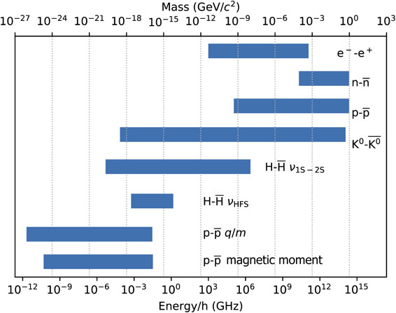
(Color online) Comparisons of several tests of CPT symmetry on the energy scale. Bar’s right end, energies of the measured quantities; length of bar, relative precision of the CPT test except for the neutral kaon case (see §2.3); bar’s left end, sensitivity in an absolute energy scale. The values are from PDG37) except for the $\overline{\text{H}}$ results for HFS145) and 1S-2S.107) In the case of the $\overline{\text{p}}$ charge-to-mass ratio,146) the length of the bar is well defined, while the right end is the cyclotron frequency, which is proportional to the magnetic field.147) For a more rigorous comparison, one possible way is to convert to the upper limit of the SME coefficients.126)
As discussed in §2.4, direct measurements of the gravitational interaction between antimatter and matter are the other key topics of the cold antimatter research discussed in this article. Gravity is described by general relativity, a classical theory invented by Einstein in 1915 when antimatter was not known even conceptually (Dirac’s relativistic theory which discovered “antielectron” (positron) was in 1928). No theoretical framework has been known until now to unify general relativity and quantum mechanics, i.e., the related topics are quite attractive also from experimentalists’ viewpoints. The equivalence principle is the foundation of general relativity, and a considerable number of experiments have been performed and are still in progress to test its validity among various forms of matter. In contrast, there has not been a single direct measurement of the gravitational interaction between matter and antimatter. Neutral antihydrogen is a unique system with which the Weak Equivalence Principle (WEP) can be directly tested for the first time with antimatter in a completely model-independent way.
In order for free-fall to be practically observable, a good guess would be to expect gΔt to be comparable to, or larger than, vT, where g is the gravitational acceleration (= 9.8 m/s2), Δt the observation time and vT a typical velocity due to thermal motion of antihydrogen atoms. Considering a possible size of the vacuum chamber for free-fall experiments of $\overline{\text{H}}$s to be ∼1 m at maximum, i.e., vTΔt ∼ 1 m, we get vT ∼ 3 m/s. The desirable temperature of $\overline{\text{H}}$ for the free-fall experiment is then estimated to be ∼1 mK or lower, which is many orders of magnitude colder than what had ever been achieved until now, and this is where each experiment squeezes an ingenious idea as explained below.
7.1. Free-fall measurements of a horizontally extracted antihydrogen beam: AEgIS.Figure 17(a) schematically shows the key idea of the AEgIS experiment to measure the gravitational force acting on $\overline{\text{H}}$s using a so-called Moire deflectometer. Let’s consider a case where a divergent $\overline{\text{H}}$ beam is injected on two subsequent gratings, and the annihilation points are recorded by the emulsion detector at the downstream end. Because of the double-grating configuration, the annihilation pattern is discretized and the corresponding trajectories are identified even when the $\overline{\text{H}}$ beam quality is not necessarily excellent. As Fig. 17(b) shows, the expected trajectories of $\overline{\text{H}}$s would be bent like the blue lines due to the gravitational force.148) By comparing the transmission pattern of slow $\overline{\text{H}}$s on the emulsion detector with the transmission pattern of light, the gravitational force can be evaluated.

(Color online) (a) Divergent antihydrogen beam impinges on two subsequent gratings (slit width of 12 µm and periodicity of 40 µm) that restrict the transmitted particles to well-defined trajectories, and eventually hit the emulsion detector. (b) In the presence of the gravitational force, the particle trajectories are bent (blue trajectories), and finally detected by an emulsion detector with a high spatial resolution.148)
For the double-grating configuration shown in Fig. 17(a) (slit height of 12 µm and a period of 40 µm, and the two gratings are separated by 25 mm), the $\overline{\text{H}}$ temperature can be two orders of magnitude higher than was crudely evaluated (∼1 mK) at the beginning of §7. This “high” temperature is, however, still a big challenge experimentally. The AEgIS experiment is going to use a dilution refrigerator to cool $\overline{\text{p}}$s down to this temperature.
The $\overline{\text{H}}$ beam necessary for the AEgIS experiment is prepared in the following way:
The goal of the first phase is to reach a precision of Δg/g ∼ 10−2.148),150)
7.2. Free-fall experiment of ultra cold $\overline{\text{H}}$: GBAR.The next experiment aimed at a direct observation of the gravitational interaction is the Gravitational Behaviour of Antihydrogen at Rest (GBAR) experiment.151) As its name tells the idea is very straightforward, $\overline{\text{H}}$s are prepared at an extremely low temperature, and they are allowed to literally free-fall, i.e., to mimic the Galileo’s Leaning Tower of Pisa experiment not with metallic balls but with the simplest antimatter, $\overline{\text{H}}$s. The final goal is to determine the gravitational force with a precision of 10−3. The key point of the GBAR experiment is therefore to invent a scheme to prepare $\overline{\text{H}}$s at extremely low temperature, which is not at all possible with the conventional antiproton cooling technique developed until now.
The key point is to produce an antihydrogen ion ($\overline{\text{H}}^{ + }$) which is made of one $\overline{\text{p}}$ and two e+s. Because an $\overline{\text{H}}^{ + }$ ion is positively charged, it can be safely co-trapped with positively charged ions and sympathetically cooled by surrounding ions which are cooled. For example, Be+ ions can be laser-cooled down to a few nano eV (∼10 µK), and so eventually $\overline{\text{H}}^{ + }$ is sympathetically cooled, too.152) Once cooled, one positron is gently photo-detached from $\overline{\text{H}}^{ + }$, and the resultant ultra-cold $\overline{\text{H}}$ starts free-falling. By measuring the annihilation time and position, the force on the $\overline{\text{H}}$ can be correctly evaluated. Photo detachment is induced by horizontally polarized laser light to minimize the vertical heatup of the resultant $\overline{\text{H}}$ by the recoil of the detaching positron. The kinetic energy of a detaching positron is planned to be ∼10−5 eV or lower.
Figure 18(a) schematically shows a procedure to prepare $\overline{\text{H}}^{ + }$, which consists of the following 4 steps:

(Color online) (a) Schematic drawing showing how to synthesize an antihydrogen ion, $\overline{\text{H}}^{ + }$. A large number of positrons are pulse-injected on the porous target from the top. Thermal positroniums (Ps) emitted are laser-excited. In coincidence with the production of Ps in excited states, pulsed antiprotons are injected into the Ps cloud to synthesize $\overline{\text{H}}^{ + }$ via two-step charge transfer processes. (b) Vertical cross section of the free-fall detector chamber. The $\overline{\text{H}}^{ + }$ ion is guided from the top and trapped by the Paul trap in the middle of the free-fall detector, and sympathetically cooled with laser-cooled Be+ ions preloaded. After cooling, one positron is laser detached, and the ultra-cold $\overline{\text{H}}$ starts its free-fall journey.151)
As shown in Fig. 18(b), an $\overline{\text{H}}^{ + }$ at a few keV is transported to the Paul trap from the top, decelerated and trapped, and then sympathetically cooled by preloaded laser-cooled Be+ ions. The Paul trap is located at the center of the free-fall detector chamber surrounded by annihilation detectors.
The other key point of the GBAR experiment is how to prepare 1010 positroniums so that they are ready to be shot by a few keV $\overline{\text{p}}$s delivered from ELENA every 100 s. A typically available 22Na source gives ∼109 Bq, resulting in at best 107 slow e+s/s, i.e., an order of magnitude less than is necessary. The GBAR experiment developed a strong positron source based on a 9 MeV electron accelerator. The electron beam energy was selected so that no persistent radioactive activation would take place in the target zone. Bremsstrahlung γ rays produced by the electron beam hitting a tungsten plate are converted to positrons via pair production processes. An electron beam power of 2 kW is expected to give 108 slow e+s/s.
As one of possible future programs, the formation of gravitational quantum states of $\overline{\text{H}}$ is proposed by combining a horizontal reflection surface and Earth’s gravity,153),154) which is expected to reduce the statistical uncertainty and also to have the ability to search, for instance, fifth forces and non-Newtonian gravity. The idea to form gravitational quantum states had already been realized with ultra-cold neutrons.155)
7.3. Free-fall of $\overline{\text{H}}$s in a magnetic trap: ALPHA-g.The ALPHA experiment has recently widened their physics program, also to include gravitational interaction research by constructing a new vertical magnet to trap and to make a free-fall experiment of $\overline{\text{H}}$s.156) A strong point of the ALPHA-g experiment is it has already established a highly efficient and reliable technique to trap $\overline{\text{H}}$s as discussed in §6.1. The $\overline{\text{H}}$ temperature would be a fraction of a Kelvin, and so adiabatic and laser157) cooling techniques are proposed to further reduce the $\overline{\text{H}}$ temperature down to a sub-50 mK range, corresponding to a $\overline{\text{H}}$ speed of a couple of ten m/s. This temperature is in between those targeted by the AEgIS and GBAR experiments. It is proposed to evaluate WEP with a precision of ∼10−2 in the first phase.
A light-pulse atom interferometer is also envisaged for the future, which could reach a precision as high as one part-per-million.158)
Encouraged by a recent improvement in the storing time,131) ideas to transport $\overline{\text{p}}$s to other facilities are becoming increasingly a reality. The antiProton Unstable Matter Annihilation (PUMA) experiment proposed to transport $\overline{\text{p}}$s to the ISOLDE facility in the same Meyrin campus of CERN, and to mix $\overline{\text{p}}$s with unstable nuclei delivered by ISOLDE to form antiprotonic atoms made of unstable nuclei (see, https://www.dropbox.com/s/3kimkzg8r6feumr/PUMA_SPSCproposal_submitted.pdf?dl=0).
Once a long distance transport of $\overline{\text{p}}$s is realized, various new research subjects, which would otherwise not be possible, will emerge, e.g., a CPT symmetry test comparing the spectroscopic properties of μ+$\overline{\text{p}}$ and μ−p (see §8.3) by transporting $\overline{\text{p}}$s to a muon facility. Further, cyclotron frequency measurements of protons and antiprotons at different altitudes126) are proposed to search for a gravitational redshift of matter and antimatter (see also Ref. 15). This idea can be extended to measure cyclotron frequencies of $\overline{\text{p}}$s on a satellite under a free-falling condition.
The PUMA project consists of three phases:
Actually, antiprotonic atoms were studied by injecting energetic antiprotons into various isotope-enriched stable targets.159),160) Figure 19 shows an example of antiprotonic X-ray spectra from $\overline{\text{p}}$48Ca. A series of intense peaks are identified as Yrast line transitions (Δn = 1) as low as the 6→5 transition. However, no signature could be seen at the energy of the 5→4 transition, which strongly indicates that the $\overline{\text{p}}$ annihilates before the 5→4 transition. Considering that the Yrast states are circular (l ∼ n − 1), annihilation takes place with one of the nucleons near to the surface of 48Ca nuclei when the orbital size of $\overline{\text{p}}$ (n ∼ 5) becomes comparable to the nucleus. If, on the other hand, $\overline{\text{p}}$ is in an ns state even if n ≫ 1, it would immediately annihilate with one of the nucleons of the 48Ca nucleus.

The idea to transport $\overline{\text{p}}$s for a long distance had already been discussed in 2004161),162) also considering to study unstable nuclei by measuring the number of π+s and π−s emitted during $\overline{\text{p}}$ annihilation. In this way, the annihilation partner (proton or neutron) in the nuclei can be pinned down (The storing time of $\overline{\text{p}}$s at that time was reported to be 3.4 months129)). Figure 20 shows a possible scheme of how to efficiently combine $\overline{\text{p}}$s and A+s.162) Actually, this configuration is the same as that of a nested trap adopted to successfully synthesize $\overline{\text{H}}$ atoms (see §5.1). The antiprotonic atom formation process is again a three-body recombination process involving $\overline{\text{p}}$, A++, and one of the outermost electrons of A+. A theoretical simulation predicts that the exotic atom formation cross section between $\overline{\text{p}}$ and a singly charged ion with bound electron(s)163) is similar to that between $\overline{\text{p}}$ and a neutral atom.164) On the other hand, the recombination cross section with a highly charged ion would be strongly suppressed, if not zero, except for some peculiar conditions, e.g., an inverse Auger process ($\overline{\text{p}} + A^{\text{q} + } \to \overline{\text{p}}A^{\text{q} + *} \to \overline{\text{p}}A^{\text{q} + 1} + \text{e}^{ - }$), which is similar to a so-called Resonant Transfer and Excitation (RTE) process.165) Considering these, it would be preferable to prepare unstable nuclei as singly charged ions for the efficient formation of antiprotonic atoms.

(Color online) Possible configuration of the nested trap to synthesize antiprotonic ions.162) Electrons are stored together with antiprotons to cool A+ ions so that the recombination efficiencies are enhanced.
An exotic atom $\overline{\text{p}}A$+ is formed in its principal quantum number, $n_{\overline{\text{p}}}\ \sim \ \sqrt{m_{r}/m_{\text{e}}} $, if $\overline{\text{p}}$ and A or A+ are mixed, where $m_{\text{r}} = m_{A}m_{\overline{\text{p}}}/(m_{A} + m_{\overline{\text{p}}})$ (see §6.3), and the $\overline{\text{p}}$ cascades down firstly via Auger transitions, and then via radiative transitions emitting antiprotonic X-rays. During these cascading down processes, the $\overline{\text{p}}$ annihilates with one of the nucleons of the nucleus as soon as the atomic state of the antiprotonic atom has l = 0 (an s state) and/or low l components, If, on the other hand, $\overline{\text{p}}$ is in a Yrast state, it cascades down step by step (i.e., Δn = 1) until the circular orbit starts to overlap with the periphery of the nucleus, and then annihilates with one of the nucleons near to the surface of the nucleus. It would be interesting to measure the charge distribution of π±s emitted during $\overline{\text{p}}$ annihilations in coincidence with antiprotonic X-rays, which would provide detailed information concerning the proton and neutron radial distributions in unstable nuclei. This idea can be applicable to stable nuclei, which would be realized by injecting a well-collimated atomic/molecular beam along the axis of an antiproton trap. The target density can be much higher than that of the unstable nuclei, but is still low enough to avoid Stark-mixing and annihilation induced by neighboring atoms. This experiment can be performed on site in the AD hall.
8.2. Antimatter chemistry.Once a large number of $\overline{\text{H}}$ atoms are available, an “antimatter chemistry” would emerge by inventing ways to synthesize $\overline{\text{H}}_{2}^{ - }$, $\overline{\text{H}}_{2}$, and beyond. The formation of $\overline{\text{H}}^{ + }$, discussed in §7.2, would have actually been a whistling arrow in this direction. A new and more sensitive CPT test with $\overline{\text{H}}_{2}^{ - }$ has been proposed for measuring ro-vibrational transitions.166)
The field of antimatter chemistry would reach a new stage once cold $\overline{\text{d}}$s become available (see §8.4), which would allow syntheses not only of antideuterium ($\overline{\text{D}} = \overline{\text{d}}\text{e}^{ + }$), but also of antimolecular ions, such as $\overline{\text{H}}\,\overline{\text{D}}^{ - }( = \overline{\text{p}}\overline{\text{d}}\text{e}^{ + })$, $\overline{\text{D}}^{-}_{2}( = \overline{\text{d}}\,\overline{\text{d}}\text{e}^{ + })$, as well as antimolecules, such as $\overline{\text{H}}\,\overline{\text{D}}( = \overline{\text{d}}\overline{\text{p}}\text{e}^{ + }\text{e}^{ + }),\overline{\text{D}}_{2}( = \overline{\text{d}}\,\overline{\text{d}}\text{e}^{ + }\text{e}^{ + })$, etc.
8.3. Muonic hydrogen vs muonic antihydrogen.An interesting future subject is to replace e−/e+ of H/$\overline{\text{H}}$ by μ−/μ+ and to conduct high-precision spectroscopy of muonic hydrogen (μ−p) and muonic antihydrogen (μ+$\overline{\text{p}}$).167) A muon is a point-like particle ∼200 times more massive than e−/e+, and, accordingly, μ−p and μ+$\overline{\text{p}}$ are ∼200 times smaller than H and $\overline{\text{H}}$. This system could probe the proton and antiproton with much higher sensitivity. Such an experiment could be realized by transporting $\overline{\text{p}}$s to a proper muon facility.
Actually, μ−p was synthesized by injecting a low energy μ− beam in an H2 gas cell, and its 2s-2p transition frequency, ν2s–2p, was measured in 2010, resulting in ν2s–2p = 49,881.88(76) GHz.168) The proton charge radius, evaluated from this spectroscopic result, was rp = 0.84184(67) fm, which was 5.0 standard deviations from the CODATA value of 0.8768(69) fm that was evaluated from electron scattering experiments at that time. This large deviation was a big news in the community.7 The 2s-2p transition of μ+$\overline{\text{p}}$ would of course be an interesting target for a comparison.
Regarding μ+$\overline{\text{p}}$ formation, e.g., a charge exchange collision like $\overline{\text{p}} + \mu ^{ + }\text{e}^{ - } \to \mu ^{ + }\overline{\text{p}} + \text{e}^{ - }$ could reasonably be applied. The production of μ+e−s can be realized by injecting slow μ+ particles in various solid materials like silica aerogel with a production efficiency of 0.03 μ+e−/μ+,169) a similar scheme to produce positroniums as discussed in §7.1 and §7.2.
8.4. Antideuteron production.It would be quite attractive for cold antimatter research if antideuterons ($\overline{\text{d}}$s) become available, which would enable high-precision antimatter research to be conducted involving antineutrons ($\overline{\text{n}}$) for the first time.8
D. Möhl and his colleagues proposed an elegant scheme to produce and to accumulate $\overline{\text{d}}$s using a mirror reaction of p + p → d + π+, i.e., $\overline{\text{p}} + \overline{\text{p}} \to \overline{\text{d}} + \pi ^{ - }$ by combining two storage rings with a common straight section so that $\overline{\text{p}}$ beams with two different momenta collide in the straight section to produce $\overline{\text{d}}$s.171) An excellent idea concerning such a double storage ring scheme is to tune the momenta of two $\overline{\text{p}}$ beams so that the momentum of the resulting $\overline{\text{d}}$, $\vec{P}_{{\bar{\text{d}}}}$, is the same as one of the $\overline{\text{p}}$ momentum, $\vec{P}_{\overline{\text{p}}}$. In this way, $\overline{\text{d}}$s are automatically accumulated in the ring. Once $\overline{\text{d}}$s are accumulated, exactly the same procedures for cooling, deceleration, and trapping developed for $\overline{\text{p}}$s can be applied.
The developments of cold antimatter research with antiprotons and antihydrogen atoms during the last twenty years or so have been reviewed primarily focusing on activities at AD, which started from 2000 until now together with various promising subjects in the near future. It is impressive to recall that various milestones have been marked. This includes the synthesis, trapping, and high-precision spectroscopy of antihydrogen atoms, as well as the world record competition of antiproton and proton magnetic moments, in addition to the high-precision laser spectroscopy of antiprotonic helium. The 1S-2S transition energy of antihydrogen atoms has been compared with the hydrogen case, which confirmed the CPT symmetry with <10−20 GeV/c2, which is more than an order of magnitude higher in precision than the K0-$\overline{\text{K}^{0}}$ mass difference of <4 × 10⁻¹⁹ GeV/c2. It is also noted that the magnetic moment of $\overline{\text{p}}$, which is available only artificially, was once determined with a higher precision than that of p at that time, the most abundant matter in the universe.
Three experiments are seriously chasing to directly measure the gravitational interaction between antimatter (antihydrogen) and matter (Earth), which is increasingly becoming a reality due to various technical developments to cool $\overline{\text{H}}$s. Further, a new experiment to use antiprotons to probe the structures of unstable nuclei is about to start.
All of the subjects discussed in this review would accelerate the pace of their progress once ELENA starts to provide one to two orders of magnitude more antiprotons from 2021. Our understanding of nature would definitely be deepened first quantitatively, and then qualitatively, in parallel with an increasing overlap with other fundamental physics fields. The search for interactions of antiprotons with axion-like dark matter particle would have been the first such example (see §6.2), and should be extended to various quantities and interactions.
The author has been studying cold antimatter physics for more than 30 years, since 1989 via the PS204 experiment during the LEAR time, and then the whole AD period until now. The author would like to deeply thank all colleagues who have worked together for their inspiring discussions and for their great work not only concerning ASACUSA and BASE, but also many colleagues from other experiments, ATHENA, ALPHA, and GBAR, as well as ATRAP and AEgIS. The author would like to thank CERN, specifically the Antiproton Decelerator (AD) team and the Radio Frequency (RF) team, for their hard work and great support. The author gives deep thanks for strong support to the cold antimatter research discussed here by Grant-in-Aids of the Ministry of Education, Culture, Sports, Science and Technology, the Creative Scientific Research (10P0101), the Specially Promoted Research (19002004 & 24000008) as well as the International Scientific Research Program (01044033, 03044039 & 07044067) and the Scientific Research (A) (06402015). Sincere thanks are given to various intra-RIKEN programs, like the Special Research Projects for Basic Science, the Pioneering Project, Strategies for a Global RIKEN Project, for their timely and crucial support.
Edited by Toshimitsu YAMAZAKI, M.J.A.
Correspondence should be addressed: Y. Yamazaki, RIKEN, 2-1 Hirosawa, Wako, Saitama 351-0198, Japan (e-mail: yasunori@riken.jp).
1 It would also be interesting to pursue a new electromagnetic accelerator with a much shorter wavelength, which can in principle make the whole size of the accelerator much smaller (private communication from Minamide, H. (RIKEN) and Ref. 17).
2 The C/P/T/CP/CT/PT/CPT properties of these operators are given in Table P46 (p. 107) of Ref. 33.
3 Beam cooling in the storage ring had a big impact in the elementary particle physics communities, such as the discovery of W and Z bosons. At the same time a new research field emerged e.g., in the atomic physics community. Actually, cooled ions continuously collide with cooling electrons with a very small relative velocity, i.e., electron–ion collisions with the collision energy as low as ∼100 µeV are realized in storage rings, which is otherwise practically impossible. Various cooler rings, even electrostatic ones, have been constructed and are still in operation primarily in Europe (e.g., at GSI). An interesting example of knock-on effects to other fields (see e.g., Ref. 49).
4 Actually, the antiproton cooling scheme described here was originally developed by the later ATRAP group69),70) already in 1989 during the LEAR time (see Fig. 2), and is now the standard technique to cool antiprotons adopted by all the experiments at the AD.
5 This value was later slightly modified to be $\mu _{\overline{\text{p}}} = - 2.7928473443(46)$ μN.126)
6 Detailed experimental procedures may be re-examined later (private communication from Obertelli, A.).
7 The CODATA value in 2018 was renewed to be 0.8414(19) fm, which is closer to that extracted from the μ−p experiment.
8 Although an $\overline{\text{n}}$ beam has been obtained by a charge exchange reaction, like $\overline{\text{p}} + \text{p} \to \overline{\text{n}} + \text{n}$, for a broad energy range170) (3.6 × 10⁻⁵ $\overline{\text{n}}/\overline{\text{p}}$ for 406 MeV/c $\overline{\text{p}}$), it is quite difficult to manipulate for high-precision measurements because it is neutral.

Yasunori Yamazaki was born in 1949 in Osaka, Japan. He graduated from Osaka University, Department of Physics, Faculty of Science, and then went on to Graduate School of Engineering, and was awarded the Doctor degree in 1978. He worked at Tokyo Institute of Technology from 1978 until 1988, and then at the University of Tokyo until 2010. From 1997, he was joint-appointed as the Chief Scientist of RIKEN leading the Atomic Physics Laboratory until 2010, and continued his research carrier as the Distinguished Senior Scientist till 2015. He was in parallel appointed as Research Strategy Advisor (deputy Executive Research Director) of RIKEN from 2014 until 2019.
He has been an experimental physicist working on a couple of different topics, such as fundamental physics (including the CPT symmetry and WEP (Weak Equivalence Principle) tests), employing cold antiprotons and antihydrogen atoms, non-neutral plasma physics, and atomic collision physics involving highly charged ions in the energy range from eV to GeV.
To pursue the antiproton and antihydrogen research, he organized an international group, the ASACUSA-Cusp collaboration, at CERN. He also joined the ALPHA and GBAR collaborations at CERN. For these contributions, he was elected as a Fellow of the American Physical Society in 2010, and he received the 15th Matsuo Foundation Hiroshi Takuma Memorial Award in 2011 and the 52nd Toray Science and Technology Prize in 2012.